P Systems with Evolutional Communication and Division Rules

Abstract

A widely studied field in the framework of membrane computing is computational complexity theory. While some types of P systems are only capable of efficiently solving problems from the class P, adding one or more syntactic or semantic ingredients to these membrane systems can give them the ability to efficiently solve presumably intractable problems. These ingredients are called to form a frontier of efficiency, in the sense that passing from the first type of P systems to the second type leads to passing from non-efficiency to the presumed efficiency. In this work, a solution to the SAT problem, a well-known NP-complete problem, is obtained by means of a family of recognizer P systems with evolutional symport/antiport rules of length at most (2,1) and division rules where the environment plays a passive role; that is, P systems from $\widehat{\mathcal{CDEC}}(2,1)$. This result is comparable to the one obtained in the tissue-like counterpart, and gives a glance of a parallelism and the non-evolutionary membrane systems with symport/antiport rules.

1. Introduction

Membrane computing is a bio-inspired paradigm of computation, based on the structure and behavior of living cells. Introduced in 1998 by G. Păun [1], giving birth to devices known as membrane systems or P systems. There are several different types of P systems, but three of them are specially studied: cell-like membrane systems [1], whose tree-like structure characterizes the relation between its regions; tissue-like membrane systems [2], defined as a set of cells that can interact between them and with the environment, and neural-like membrane systems [3], having an explicitly defined directed graph as a relation of the neurons through synapses. The last paradigm is being intensely studied in practical applications, and different variants have been created to their use in different fields [4,5,6] The paradigm of membrane computing is very wide, covering topics from theory [7,8] to applications [9,10,11], dedicating a branch to simulators and in silico implementations [12].

A widely studied question in this framework from the very beginning is which kind of problems can be solved by means of membrane systems. Membrane systems can differ in the type of objects with which they can compute (e.g., symbols, strings, matrices), the type of relation between the regions (e.g., hierarchical structure, directly connected membranes, cells implicitly connected by the rules) and the rules governing the computation of the system (e.g., object evolution rules, symport/antiport rules, division rules), among others. This variety of ingredients can change not only the type of problem that a P system can solve, but how efficiently can it solve a certain problem. More precisely, decision problems are usually studied in the field of computational complexity theory in order to classify them in complexity classes that contain problems that can be solved with a similar amount of computational resources [13].

Recognizer membrane systems [14] are P systems with certain ingredients, such as two special objects $\mathtt{yes}$ and $\mathtt{no}$, and requisites, such as all the computations halt and return the same result. The design of a family of recognizer membrane systems of a certain type $\mathcal{R}$ solving certain decision problems can reveal which kind of problems can be solved efficiently by means of that class of P systems.

A widely studied type of membrane systems in the field of computational complexity theory is the framework of tissue P systems with symport/antiport rules. In [15], a polynomial-time solution to $\mathtt{SAT}$ was designed by means of a family of recognizer tissue P systems with symport/antiport rules of length at most five and division rules. In this type of P system, the length is defined as the number of objects implied in the symport/antiport rules of the system (e.g., the length of the rule $(i,u/v,j)$ is $\left|u\right|+\left|v\right|$). This result was eventually improved in [16], where the maximum number of objects implied in a communication rule was two. If only one object was allowed in communication rules, then only tractable problems could be efficiently solved, as demonstrated in [17]. A similar frontier of efficiency was found by using separation rules instead of division rules in [18,19], but in this case, the frontier is from passing of communication rules of length at most two to length at most three, instead of passing from one to two. Some results about their relative environmentless counterparts were demonstrated in [20,21]. Symport/antiport rules were first introduced in tissue-like membrane systems, but later used in cell-like membrane systems, where results were surprisingly similar [22,23,24,25,26,27], giving a glance of the similarity of using both tree-like and directed graph structures.

In [28], tissue P systems with evolutional symport/antiport rules were introduced, including in communication rules the capability to evolve the objects while traveling from one region to another one. In this type of P system, two different definitions of length can be cited: On the one hand, the length of an evolutional communication rule can be defined with a single number that is related with the number of objects in the whole rule (e.g., in the rule ${\left[u{\left[v\right]}_j\right]}_i⟶{\left[v^{\prime }{\left[u^{\prime }\right]}_j\right]}_i$ is $\left|u\right|+\left|v\right|+|u^{\prime }|+|v^{\prime }|$); on the other hand, the length can be defined as a pair of numbers concerning the number of objects in the left-hand side and the right-hand side of the evolutional communication rules of the system (e.g., the length of the rule ${\left[u{\left[v\right]}_j\right]}_i⟶{\left[v^{\prime }{\left[u^{\prime }\right]}_j\right]}_i$ is $\left(\right|u|+|v|,|u^{\prime }|+|v^{\prime }\left|\right)$). In [29], several new results were presented, publishing some improvements from [28,30,31,32]. More precisely, in [32] an efficient family of tissue P systems with evolutional communication rules of length at most $(2,1)$ and division rules using the environment as an active agent of the system solving the $\mathtt{SAT}$ problem is presented. In this work, we investigate the role of evolutional communication rules in cell-like membrane systems that use division rules as exponential workspace-generating rules, and letting the environment as a mere agent that only receives the corresponding answer of the system.

The rest of the paper is structured as follows: Section 2 is dedicated to introducing some terms used throughout the work. In the next section, cell P systems with evolutional symport/antiport rules and division rules are defined, and their recognizer versions are introduced. Section 4 and Section 5 are devoted to present a solution to the problem $\mathtt{SAT}$ by means of a family of P systems with evolutional communication rules and division rules of length at most $(2,1)$, and to prove the correctness of the solution. Finally, in Section 6 the results of this paper are discussed, and comparatives with other classes of P systems are given, and some open research lines are proposed, besides a description of the work in progress.

2. Preliminaries

In this section, some concepts that will be used throughout the paper will be defined. The reader can find expanded and deeper information about formal languages and membrane computing in [8,33].

An alphabet is a non-empty (finite) set, whose elements are usually called symbols. A string over $\Gamma$ is a ordered finite succession of elements from $\Gamma$. We denote the empty string by $\lambda$.

Given two sets A and B, the relative complement$A\backslash B$ is defined as $A\backslash B=\{x\in A\mid x\notin B\}$. For each set A, we denote by $\left|A\right|$ the cardinal (number of elements) from A.

A multiset can be described explicitly as follows: $\{(a_1,\mathcal{M}\left(a_1\right)),\dots ,(a_n,\mathcal{M}\left(a_n\right))\}$, and the notation $\mathcal{M}=a_1^{\mathcal{M}\left(a_1\right)}\dots a_n^{\mathcal{M}\left(a_n\right)}$ will be used. The cardinal of a multiset $\mathcal{M}$ over $\Gamma =\{a_1,\dots ,a_n\}$ is defined as $\left|\mathcal{M}\right|=\mathcal{M}\left(a_1\right)+\dots +\mathcal{M}\left(a_n\right)$. We denote by $M_f(\Gamma )$ the set of all the finite multisets over $\Gamma$, and $M_f^{+}(\Gamma )=M_f(\Gamma )\backslash \{\varnothing \}$

Given two multisets $M_1$ and $M_2$ over $\Gamma$, the union of the multisets, denoted as $M_1\cup M_2$ or $M_1+M_2$, is the application over $\Gamma$ defined as: for each $a\in \Gamma$, $(M_1\cup M_2)\left(a\right)=M_1\left(a\right)+M_2\left(a\right)$. A multiset $M_1$ is included in $M_2$, and it is denoted by $M_1\subseteq M_2$, if $M_1\left(a\right)\le M_2\left(a\right)$ for each $a\in \Gamma$.

3. P Systems with Evolutional Communication and Division Rules

In this section, the framework of cell-like membrane systems where evolutional communication rules and division rules are used is introduced.

Definition 1.

A P system with evolutional symport/antiport rules and division rules of degree $q\ge 1$ is a tuple

$$\Pi =\left(\Gamma ,\mathcal{E},\mu ,{\mathcal{M}}_1,\dots ,{\mathcal{M}}_q,{\mathcal{R}}_1,\dots ,{\mathcal{R}}_q,i_{out}\right)$$

where:

• Γ is a finite (working) alphabet;
• $\mathcal{E}\subseteq \Gamma$ is the environment alphabet;
• μ is a rooted tree structure;
• ${\mathcal{M}}_1,\dots ,{\mathcal{M}}_q$ are the initial multisets of the membranes;
• ${\mathcal{R}}_1,\dots ,{\mathcal{R}}_q$ are the rules of the membranes of the system of the following form:

  –

  ${\left[u{\left[\right]}_j\right]}_i⟶{\left[{\left[u^{\prime }\right]}_j\right]}_i$, with $0\le i,j\le q,i\ne j,u\in M_f^{+}(\Gamma ),u^{\prime }\in M_f(\Gamma )$; in the case that $i=0$, then u must contain at least one object from $\Gamma \backslash \mathcal{E}$ (evolutional send-in symport rules);

  –

  ${\left[{\left[u\right]}_j\right]}_i⟶{\left[u^{\prime }{\left[\right]}_j\right]}_i$, with $0\le i,j\le q,i\ne j,u\in M_f^{+}(\Gamma ),u^{\prime }\in M_f(\Gamma )$ (evolutional send-out symport rules);

  –

  ${\left[u{\left[v\right]}_j\right]}_i⟶{\left[v^{\prime }{\left[u^{\prime }\right]}_j\right]}_i$, with $0\le i,j\le q,i\ne j,u,v\in M_f^{+}(\Gamma ),u^{\prime },v^{\prime }\in M_f(\Gamma )$ (evolutional antiport rules);

  –

  ${\left[a\right]}_i⟶{\left[b\right]}_i{\left[c\right]}_i$, with $1\le i\le q,i\notin \{i_{out},i_{skin}\},a,b,c\in \Gamma$, being $i_{skin}$ the label of the skin membrane (division rules).

• $i_{out}\in \{0,1,\dots ,q\}$ is the output region of the system.

A P system with evolutional symport/antiport rules and division rules of degree $q\ge 1$ can be seen as a set of q membranes biyectively labelled by $1,\dots ,q$ organized in the rooted tree structure $\mu$, whose root node is the skin membrane, and such that (a) $\mathcal{E}$ represents the set of objects that are situated in the environment an arbitrary number of times; (b) ${\mathcal{M}}_1,\dots ,{\mathcal{M}}_q$ represents the initial multisets situated in the q membranes of the system; (c) $i_{out}$ is a distinguished region i that will encode the output of the system. The term region i will be used to denote the membrane i, in case $1\le i\le q$, and to the environment in the case $i=0$ or $i=env$. We will use $env$ and 0 indistinguishably as the label of the environment. If $\mathcal{E}=\varnothing$, it is usually omitted from the tuple.

A configuration at an instant t of such a system is described by the membrane structure of the P system at the instant t, the multisets of objects from $\Gamma$ in each membrane at that instant and the multiset of objects from $\Gamma \backslash \mathcal{E}$ situated in the environment. The initial configuration of $\Pi =\left(\Gamma ,\mathcal{E},\mu ,{\mathcal{M}}_1,\dots ,{\mathcal{M}}_q,{\mathcal{R}}_1,\dots ,{\mathcal{R}}_q,i_{out}\right)$ is $(\mu ,{\mathcal{M}}_1,\dots ,{\mathcal{M}}_q,\varnothing )$.

A evolutional send-in symport rule is applicable to a configuration ${\mathcal{C}}_t$ at an instant t if there exists a region labelled by i that has at least a child membrane labelled by j and that it contains the multiset u of objects. The execution of such a rule ${\left[u{\left[\right]}_j\right]}_i⟶{\left[{\left[u^{\prime }\right]}_j\right]}_i$ in ${\mathcal{C}}_t$ consumes the objects of u from such a region i, and it produces the multiset of objects $u^{\prime }$ in the child membrane j in ${\mathcal{C}}_t$.

A evolutional send-out symport rule is applicable to a configuration ${\mathcal{C}}_t$ at an instant t if there exists a region labelled by i that has at least a child membrane labelled by j and the child membrane contains the multiset u of objects. The execution of such a rule ${\left[{\left[u\right]}_j\right]}_i⟶{\left[u^{\prime }{\left[\right]}_j\right]}_i$ in ${\mathcal{C}}_t$ consumes the objects of u from such a region j, and it produces the multiset of objects $u^{\prime }$ in the child membrane i in ${\mathcal{C}}_t$.

A evolutional antiport rule is applicable to a configuration ${\mathcal{C}}_t$ at an instant t if there exists a region labelled by i that contains a multiset of objects u and it has at least a child membrane labelled by j and the child membrane contains the multiset v of objects. The execution of such a rule ${\left[u{\left[v\right]}_j\right]}_i⟶{\left[v^{\prime }{\left[u^{\prime }\right]}_j\right]}_i$ in ${\mathcal{C}}_t$ consumes the objects of u from such a region j and objects from v from such a region i, and it produces the multiset of objects $u^{\prime }$ in that membrane i and the multiset of objects $v^{\prime }$ in that membrane j in ${\mathcal{C}}_t$.

A division rule is applicable to a configuration ${\mathcal{C}}_t$ at an instant t if there exists a region labelled by i that contains an object a. The execution of such a rule ${\left[a\right]}_i⟶{\left[b\right]}_i{\left[c\right]}_i$ in ${\mathcal{C}}_t$ consumes the object a from the membrane i, the membrane is duplicated with its contents included, and objects b and c are produced one in each new membrane created in ${\mathcal{C}}_t$.

As in tissue P systems with evolutional symport/antiport rules, two definitions of length (or size) can be described. On the one hand, the length of a evolutional communication rule $r\equiv {\left[u{\left[v\right]}_j\right]}_i⟶{\left[v^{\prime }{\left[u^{\prime }\right]}_j\right]}_i$ can be $length\left(r\right)=\left(\right|u|+|v|+|u^{\prime }|+|v^{\prime }\left|\right)$; on the other hand, it can be described as a pair $lengt{h}^{\prime }\left(r\right)=\left(\right|u|+\left|v\right|,|u^{\prime }|+|v^{\prime }\left|\right)$. The first description corresponds with the sum of the cardinalities of all the multisets in the rule, while the second definition corresponds with the pair such that the first component corresponds with the sum of cardinalities of the left-hand side of the rule (LHS), and the second component corresponds with the sum of the cardinalities of the right-hand side of the rule (RHS). If r is a symport rule, then $\left|v\right|=|v^{\prime }|=0$ or $\left|u\right|=|u^{\prime }|=0$.

We say that a configuration ${\mathcal{C}}_t$ of a P system with evolutional communication rules and division rules $\Pi$ produces a configuration ${\mathcal{C}}_{t+1}$ in a transition step, denoted by ${\mathcal{C}}_t{\Rightarrow }_{\Pi }{\mathcal{C}}_{t+1}$ and we say that ${\mathcal{C}}_{t+1}$ is a next configuration of ${\mathcal{C}}_t$ if we can pass from ${\mathcal{C}}_t$ to ${\mathcal{C}}_{t+1}$ applying the rules of $\Pi$ according to the following principles:

• At most one rule can be applied to each object of each membrane (selected in a non-deterministic way).
• For each membrane i, either evolutional communication rules ${\left[u{\left[v\right]}_j\right]}_i⟶{\left[v^{\prime }{\left[u^{\prime }\right]}_j\right]}_i$ or a single division rule ${\left[a\right]}_i⟶{\left[b\right]}_i{\left[c\right]}_i$ can be applied. In the case of applying evolutional communication rules at configuration ${\mathcal{C}}_t$, they would be selected in a non-deterministic, parallel and maximal way; that is, all the objects in the membrane i that can fire a rule, will fire it. In the case that a division rule ${\left[a\right]}_i⟶{\left[b\right]}_i{\left[c\right]}_i$ is applied, it will be selected in a non-deterministic way. It can be seen as the division rule blocks the communication of the membrane with its corresponding parent membrane. All the rules are applied in an atomic way, but in order to be precise, it can be that two microsteps are executed: first, all the evolutional communication rules are executed, and then division rules are executed. It is worth taking this into account since a membrane i being divided can still communicate with its inner membranes in the same transition step.

A configuration ${\mathcal{C}}_t$ is a halting configuration if no rules can be applied to such configuration at an instant t.

A computation $\mathcal{C}$ of a P system $\Pi$ can be described as a tuple $\mathcal{C}=({\mathcal{C}}_0,{\mathcal{C}}_1,\dots )$, where each configuration ${\mathcal{C}}_{t+1}$ can be obtained from ${\mathcal{C}}_t$, except for the initial configuration ${\mathcal{C}}_0$. We say that $\mathcal{C}$ is a halting computation of length $n+1$ if the configuration ${\mathcal{C}}_n$ is a halting configuration.

Recognizer membrane systems were introduced in [14] as a way to solve decision problems. We define here recognizer P systems with evolutional communication rules and division rules.

Definition 2.

A recognizer P system with evolutional communication rules and division rules of degree $q\ge 1$ is a tuple $(\Pi ,\Sigma ,i_{in})$, where:

• $\Pi =\left(\Gamma ,\mathcal{E},\mu ,{\mathcal{M}}_1,\dots ,{\mathcal{M}}_q,{\mathcal{R}}_1,\dots ,{\mathcal{R}}_q,i_{out}\right)$is a P system with evolutional communication rules and division rules of degree q, with$\{\mathtt{yes},\mathtt{no}\}\subseteq \Gamma \backslash \mathcal{E}$two distinguished objects that will represent the output of the system, and ${\mathcal{M}}_i\subseteq \Gamma \backslash \Sigma$ for $1\le i\le q$;
• $\Sigma \subseteq \Gamma \backslash \mathcal{E}$is the input alphabet;
• $i_{in}\in \{1,\dots ,q\}$is the label of the input membrane;
• $i_{out}=0$;
• All the computations of Π halt.
• If$\mathcal{C}$is a computation of Π, then either an object $\mathtt{yes}$ or an object $\mathtt{no}$, but not both, are sent to the environment in the last step of the computation.

Let $\Pi =\left(\Gamma ,\Sigma ,\mathcal{E},\mu ,{\mathcal{M}}_1,\dots ,{\mathcal{M}}_q,{\mathcal{R}}_1,\dots ,{\mathcal{R}}_q,i_{in},i_{out}\right)$ be a recognizer P system of this type, then for each input multiset m over $\Sigma$, we consider the system $\Pi$ with input multiset m, and we denote it by $\Pi +m$. This is characterized by the fact that the multisets associated with the initial configuration of the system is: $({\mathcal{M}}_1,\dots ,{\mathcal{M}}_{i_{in}}+m,\dots ,{\mathcal{M}}_q,\varnothing )$; that is, it is obtained from the initial configuration $({\mathcal{M}}_1,\dots ,{\mathcal{M}}_{i_{in}},\dots ,{\mathcal{M}}_q,\varnothing )$ of $\Pi$, by adding the multiset m to ${\mathcal{M}}_{i_{in}}$.

We define then a $Output\left(\mathcal{C}\right)$ function whose domain is the set of computations of $\Pi$. Such a function will formalize the results or outputs of the system. If $\mathcal{C}$ is a computation of the system $\Pi$, then $Output\left(\mathcal{C}\right)=\mathtt{yes}$ (respectively, $Output\left(\right)=\mathtt{no}$) if the object $\mathtt{yes}$ (resp., object $\mathtt{no}$) appears in the environment associated to the halting configuration of $\mathcal{C}$, but does not appear in any other configuration of $\mathcal{C}$. A computation $\mathcal{C}$ will be called an accepting computation (respectively, a rejecting computation) if $Output\left(\mathcal{C}\right)=\mathtt{yes}$ (resp., $Output\left(\mathcal{C}\right)=\mathtt{no}$). Computations of recognizer membrane systems always halt, and will return either $\mathtt{yes}$ or $\mathtt{no}$ as a response. A recognizer membrane system with input multiset $\Pi +m$ is confluent, in the sense that all the computations give the same answer; that is, given an input multiset m, all the computations of a recognizer membrane system with input multiset $\Pi +m$ will be either accepting computations or rejecting computations.

The class of recognizer P systems with evolutional symport/antiport rules of length at most k (respectively, with length at most $(k_1,k_2)$) and division rules is denoted by $\mathcal{CDEC}\left(\right(k\left)\right)$ (resp., $\mathcal{CDEC}\left((k_1,k_2)\right)$). If the environment does not play an active role, we say that it is a recognizer P system with symport/antiport rules of length at most k (resp., with length at most $(k_1,k_2)$, i.e., LHS with length at most $k_1$ and RHS with length at most $k_2$) and division rules without environment, and we denote this class of systems by $\widehat{\mathcal{CDEC}}\left(k\right)$ (resp., $\widehat{\mathcal{CDEC}}(k_1,k_2)$).

In this work, a family of recognizer P systems will be used in order to solve decision problems. Let $X=(I_X,{\theta }_X)$ a decision problem. We say that X is solvable in polynomial time by means of a uniform family of recognizer P systems $\mathbf{\Pi }=\{\Pi (n):n\in \mathbb{N}\}$ of the class $\mathcal{R}$, and we denote it by $X\in {\mathbf{PMC}}_{\mathcal{R}}^{}$, if the following conditions hold:

(a)

$\mathbf{\Pi }$ is polynomially uniform by Turing machines; that is, there exists a Turing machine that constructs $\Pi \left(n\right)$ in polynomial time.

(b)

There exists a polynomial encoding $(cod,s)$ of X such that:

b.1

$\mathbf{\Pi }$ is polynomially bounded with respect to $(X,cod,s)$; that is, there exists $k\in \mathbb{N}$ such that for each $u\in I_X$, each computation of $\Pi \left(s\right(u\left)\right)+cod\left(u\right)$ runs, at most, for ${\left|u\right|}^k$ computation steps.

b.2

$\mathbf{\Pi }$ is sound and complete with respect to $(X,cod,s)$.

4. Methods

Let $\phi$ a propositional formula in CNF with n variables and p clauses. Let $s\left(\phi \right)=\langle n,p\rangle$ and $cod\left(\phi \right)$ contains $x_{i,j,0}$ if the literal $x_i$ is in the clause $C_j$, ${\overline{x}}_{i,j,0}$ if the literal $\neg x_i$ is in the clause $C_j$ and $x_{i,j,0}^{*}$ if the variable $x_i$ does not appear in the clause $C_j$. Let the function $\perp (i,j)=i\perp j=i+jn$. Then, the system $\Pi (\langle n,p\rangle )$ will be the responsible of solving $\phi$. Let

$$\Pi \left(\langle n,p\rangle \right)=(\Gamma ,\Sigma ,\mathcal{E},\mu ,{\mathcal{M}}_1,\dots ,{\mathcal{M}}_{np+5},{\mathcal{R}}_1,\dots ,{\mathcal{R}}_{np+5},i_{in},i_{out})$$

a recognizer membrane system from $\mathcal{CDEC}\left(\right(2,1))$, where:

• The working alphabet $\Gamma =\Sigma \cup \{\mathtt{yes},\mathtt{no},y_1,y_2,n_1,n_2,{\alpha }^{\prime },\#\}\cup$
  $\{a_{i,j},T_{i,j},F_{i,j},x_{i,j},{\overline{x}}_{i,j},x_{i,j}^{*}\mid 1\le i\le n,1\le j\le p\}\cup$
  $\{x_{i,j,k},{\overline{x}}_{i,j,k},x_{i,j,k}^{*}\mid 1\le i\le n,1\le j\le p,1\le k\le np+\lfloor np/2\rfloor +1\}\cup$
  $\{c_j\mid 1\le j\le p\}\cup \{{\alpha }_j\mid 1\le j\le p+1\}\cup \{{\gamma }_k\mid 0\le k\le np+2\}\cup$
  $\{{\delta }_k\mid 0\le k\le np+3\}\cup \{{\delta }_k^{\prime }\mid 0\le k\le np+1\}.$
• The input alphabet $\Sigma =\{x_{i,j,0},{\overline{x}}_{i,j,0},x_{i,j,0}^{*}\mid 1\le i\le n,1\le j\le p\}$.
• Environment alphabet $\mathcal{E}=\varnothing$.
• $\mu ={[{\left[\right]}_1{\left[\right]}_2\dots {\left[\right]}_{np}{\left[\right]}_{np+2}{\left[\right]}_{np+3}{\left[\right]}_{np+4}{\left[\right]}_{np+5}]}_{np+1}$
• $$\begin{gathered} {\mathcal{M}}_k=\varnothing ,1\le k\le np+1, \\ {\mathcal{M}}_{np+2}=\{a_{i,j}\mid 1\le i\le n,1\le j\le p\}\cup \{{\alpha }_j\mid 1\le j\le p+1\}, \\ {\mathcal{M}}_{np+3}=\left\{{\delta }_0^{\prime }\right\},{\mathcal{M}}_{np+4}=\left\{{\delta }_0\right\},{\mathcal{M}}_{np+5}=\left\{{\gamma }_0\right\}. \end{gathered}$$
• The set of rules ${\mathcal{R}}_{=}{\mathcal{R}}_1\cup \dots {\mathcal{R}}_{np+5}$ contains the following rules:

  6.1

  Rules for generating all the necessary ${\gamma }_{np+2}$ to simulate the environment.

  $\begin{array}{c}{\left[{\gamma }_k\right]}_{np+5}⟶{\left[{\gamma }_{k+1}\right]}_{np+5}{\left[{\gamma }_{k+1}\right]}_{np+5}\hfill \end{array}\mathrm{for}0\le k\le np+1$

  ${\left[{\left[{\gamma }_{np+2}\right]}_{np+5}\right]}_{np+1}⟶{\left[{\gamma }_{np+2}{\left[\right]}_{np+5}\right]}_{np+1}$

  6.2

  Rules to generate p copies of the $2^n$ possible truth assignments. For that, $2^{np}$ “partial” truth assignments will be generated. $\left.\begin{array}{c}{\left[a_{i,j}\right]}_{np+2}⟶{\left[T_{i,j}\right]}_{np+2}{\left[F_{i,j}\right]}_{np+2}\hfill \\ [[T_{i,j}{F}_{i,j^{\prime }}{{]}_{np+2}]}_{np+1}⟶{[\#{\left[\right]}_{np+2}]}_{np+1}\hfill \end{array}\right\}\mathrm{for}\begin{array}{c}1\le i\le n\hfill \\ 1\le j,j^{\prime },\le p\hfill \end{array}$

  6.3

  Rules to generate $2^{np}$ copies of $cod\left(\phi \right)$.

  $\left.\begin{array}{c}{\left[x_{i,j,0}{\left[\right]}_{i\perp j}\right]}_{np+1}⟶{\left[{\left[x_{i,j,1}\right]}_{i\perp j}\right]}_{np+1}\hfill \\ [{\overline{x}}_{i,j,0}{\left[\right]}_{i\perp j}{]}_{np+1}⟶{\left[{\left[{\overline{x}}_{i,j,1}\right]}_{i\perp j}\right]}_{np+1}\hfill \\ [x_{i,j,0}^{*}{\left[\right]}_{i\perp j}{]}_{np+1}⟶{\left[{\left[x_{i,j,1}^{*}\right]}_{i\perp j}\right]}_{np+1}\hfill \end{array}\right\}\mathrm{for}\begin{array}{c}1\le i\le n,1\le j\le p\hfill \end{array}$

  $\left.\begin{array}{c}{\left[x_{i,j,k}\right]}_{i\perp j}⟶{\left[x_{i,j,k+1}\right]}_{i\perp j}{\left[x_{i,j,k+1}\right]}_{i\perp j}\hfill \\ [{\overline{x}}_{i,j,k}{]}_{i\perp j}⟶{\left[{\overline{x}}_{i,j,k+1}\right]}_{i\perp j}{\left[{\overline{x}}_{i,j,k+1}\right]}_{i\perp j}\hfill \\ [x_{i,j,k}^{*}{]}_{i\perp j}⟶{\left[x_{i,j,k+1}^{*}\right]}_{i\perp j}{\left[x_{i,j,k+1}^{*}\right]}_{i\perp j}\hfill \end{array}\right\}\mathrm{for}\begin{array}{c}1\le i\le n\hfill \\ 1\le j\le p\hfill \\ 1\le k\le np+\lfloor np/2\rfloor \hfill \end{array}$

  $\left.\begin{array}{c}{\left[{[x_{i,j,np+\lfloor np/2\rfloor +1}]}_{i\perp j}\right]}_{np+1}⟶{\left[x_{i,j}{\left[\right]}_{i\perp j}\right]}_{np+1}\hfill \\ [[{\overline{x}}_{i,j,np+\lfloor np/2\rfloor +1}{{]}_{i\perp j}]}_{np+1}⟶{\left[{\overline{x}}_{i,j}{\left[\right]}_{i\perp j}\right]}_{np+1}\hfill \\ [[x_{i,j,np+\lfloor np/2\rfloor +1}^{*}{{]}_{i\perp j}]}_{np+1}⟶{\left[x_{i,j}^{*}{\left[\right]}_{i\perp j}\right]}_{np+1}\hfill \end{array}\right\}\mathrm{for}\begin{array}{c}1\le i\le n,1\le j\le p\hfill \end{array}$

  $\begin{array}{c}{\left[{\gamma }_{np+2}{\left[{\delta }_0^{\prime }\right]}_{np+3}\right]}_{np+1}⟶{\left[{\left[{\delta }_1^{\prime }\right]}_{np+3}\right]}_{np+1}\hfill \end{array}$

  $\begin{array}{c}{\left[{\delta }_k^{\prime }\right]}_{np+3}⟶{\left[{\delta }_{k+1}^{\prime }\right]}_{np+3}{\left[{\delta }_{k+1}^{\prime }\right]}_{np+3}\hfill \end{array}\mathrm{for}1\le k\le np$

  $\begin{array}{c}{\left[{\left[{\delta }_{np+1}^{\prime }\right]}_{np+3}\right]}_{np+1}⟶{\left[{\delta }_{np+1}^{\prime }{\left[\right]}_{np+3}\right]}_{np+1}\hfill \end{array}$

  6.4

  Rules to check which clauses are satisfied.

  $\left.\begin{array}{c}{\left[x_{i,j}{\left[T_{i,j}\right]}_{np+2}\right]}_{np+1}⟶{\left[{\left[c_j\right]}_{np+2}\right]}_{np+1}\hfill \\ [{\overline{x}}_{i,j}{\left[T_{i,j}\right]}_{np+2}{]}_{np+1}⟶{\left[{[\#]}_{np+2}\right]}_{np+1}\hfill \\ [x_{i,j}^{*}{\left[T_{i,j}\right]}_{np+2}{]}_{np+1}⟶{\left[{[\#]}_{np+2}\right]}_{np+1}\hfill \\ [x_{i,j}{\left[F_{i,j}\right]}_{np+2}{]}_{np+1}⟶{\left[{[\#]}_{np+2}\right]}_{np+1}\hfill \\ [{\overline{x}}_{i,j}{\left[F_{i,j}\right]}_{np+2}{]}_{np+1}⟶{\left[{\left[c_j\right]}_{np+2}\right]}_{np+1}\hfill \\ [x_{i,j}^{*}{\left[F_{i,j}\right]}_{np+2}{]}_{np+1}⟶{\left[{[\#]}_{np+2}\right]}_{np+1}\hfill \end{array}\right\}\mathrm{for}\begin{array}{c}1\le i\le n,1\le j\le p\hfill \end{array}$

  6.5

  Rules to check if all the clauses are satisfied by a truth assignment.

  $\begin{array}{c}{\left[{\delta }_{np+1}^{\prime }{\left[{\alpha }_{p+1}\right]}_{np+2}\right]}_{np+1}⟶{\left[{\left[{\alpha }^{\prime }\right]}_{np+2}\right]}_{np+1}\hfill \end{array}$

  $\begin{array}{c}{\left[{\left[c_j{\alpha }_j\right]}_{np+2}\right]}_{np+1}⟶{[\#{\left[\right]}_{np+2}]}_{np+1}\hfill \end{array}\mathrm{for}\begin{array}{c}1\le j\le p\hfill \end{array}$

  $\begin{array}{c}{\left[{\left[{\alpha }_j{\alpha }^{\prime }\right]}_{np+2}\right]}_{np+1}⟶{\left[n_1{\left[\right]}_{np+2}\right]}_{np+1}\hfill \end{array}\mathrm{for}\begin{array}{c}1\le j\le p\hfill \end{array}$

  6.6

  General counter.

  $\begin{array}{c}{\left[{\gamma }_{np+2}{\left[{\delta }_k\right]}_{np+5}\right]}_{np+1}⟶{\left[{\left[{\delta }_{k+1}\right]}_{np+5}\right]}_{np+1}\hfill \end{array}\mathrm{for}\begin{array}{c}0\le k\le np+2\hfill \end{array}$

  $\begin{array}{c}{\left[{\left[{\delta }_{np+3}\right]}_{np+5}\right]}_{np+1}⟶{\left[{\delta }_{np+3}{\left[\right]}_{np+5}\right]}_{np+1}\hfill \end{array}$

  6.7

  Rules to return a negative answer.

  $\begin{array}{c}{\left[n_1{\left[\right]}_{np+2}\right]}_{np+1}⟶{\left[{\left[n_1\right]}_{np+2}\right]}_{np+1}\hfill \\ [{\delta }_{np+3}{\left[n_1\right]}_{np+2}{]}_{np+1}⟶{\left[n_2{\left[\right]}_{np+2}\right]}_{np+1}\hfill \\ [[n_2{{]}_{np+1}]}_0⟶{\left[\mathtt{no}{\left[\right]}_{np+1}\right]}_0\hfill \end{array}$

  6.8

  Rules to return an affirmative answer.

  $\begin{array}{c}{\left[{\delta }_{np+3}{\left[{\alpha }^{\prime }\right]}_{np+2}\right]}_{np+1}⟶{\left[{\left[y_1\right]}_{np+2}\right]}_{np+1}\hfill \\ [[y_1{{]}_{np+2}]}_{np+1}⟶{\left[y_2{\left[\right]}_{np+2}\right]}_{np+1}\hfill \\ [[y_2{{]}_{np+1}]}_0⟶{\left[\mathtt{yes}{\left[\right]}_{np+1}\right]}_0\hfill \end{array}$

  6.9

  Input membrane $i_{in}=np+1$ and output membrane $i_{out}=0$.

In this section, the behaviour of a recognizer P system from $\mathcal{CDEC}\left(\right(2,1\left)\right)$ solving an instance $\phi$ from $\mathtt{SAT}$ is described. Let $\phi =C_1\wedge \dots \wedge C_p$ be a propositional logic formula in CNF, where $C_j=l_1\vee \dots \vee l_{r_j},l_k\in \{x_i,\neg x_i\mid 1\le i\le n\}$. Then $\phi$ will be processed by the system $\Pi \left(s\right(\phi \left)\right)+cod\left(\phi \right)$, where $s\left(\phi \right)=\langle n,p\rangle$ and $cod\left(\phi \right)=\{x_{i,j,0}\mid x_i\in C_j\}\cup \{{\overline{x}}_{i,j,0}\mid \neg x_i\in C_j\}\cup \{x_{i,j,0}^{*}\mid x_i\notin C_j\wedge \neg x_i\notin C_j\}$.

Let us note $co{d}_k\left(\phi \right)$ the set of all the elements from $cod\left(\phi \right)$ with the third subscript equal to k. Let us note $co{d}^{*}\left(\phi \right)$ the set of all the elements from $cod\left(\phi \right)$ without the third subscript.

The solution follows a brute force algorithm protocol in the framework of recognizer P systems with evolutional symport/antiport rules and division rules, and consists of the following stages:

4.1. Generation Stage

In the generation stage, different elements necessary for the rest of the computation are generated at the same time. First, in order to avoid the use of the environment to obtain $\gamma$ objects, it is necessary to use some of the synchronization protocols in [32], $2^{np+2}$ copies of the object ${\gamma }_{np+2}$ will be generated in membranes $np+5$ through the rules from 6.1. These objects will be present in the membrane $np+1$ at configuration ${\mathcal{C}}_{np+3}$. For generating the different truth assignments, objects $T_{i,j}$ and $F_{i,j}$ will represent a partial truth assignment of the variable $x_i$ in the following sense: Objects $T_{i,j}$ and $F_{i,j^{\prime }}$, with $i\ne j$, would be incompatible, since two different values would be assigned to the same variable. Therefore, in order to remove this possibility, these two objects will be removed from the system by means of the rule ${\left[{\left[T_{i,j}{F}_{i,j^{\prime }}\right]}_{np+2}\right]}_{np+1}⟶{[\#{\left[\right]}_{np+2}]}_{np+1}$. After applying these rules, only “real” truth assignments would be present in the system. In fact, there can be assignments where a variables has not been assigned any value. In this case, it will not return a false positive. For generating the different $np$ partial truth assignments, $np$ computational steps should be applied, but since rules are fired in a non-deterministic way, and the removal of these incompatible variables could be applied in between the process of generation, at most $\lfloor np/2\rfloor$ extra steps should be taken into account. Therefore, in configuration ${\mathcal{C}}_{np+\lfloor np/2\rfloor }$, membranes labelled by $np+2$ will contain all the possible truth assignments.

Besides, objects from $cod\left(\phi \right)$ will be sent into their corresponding membrane. From the second computational step, membranes $1,\dots ,np$ will be duplicated in each step until having $2^{np+\lfloor np/2\rfloor }$ copies of the corresponding object from $co{d}_{np+\lfloor np/2\rfloor }\left(\phi \right)$. These objects will be sent out to the membrane $np+1$, and therefore in the configuration ${\mathcal{C}}_{np+\lfloor np/2\rfloor +1}$, $2^{np+\lfloor np/2\rfloor }$ copies of $co{d}^{*}\left(\phi \right)$ will be present in the membrane $np+1$. In this configuration, the next stage begins.

4.2. First Checking Stage

In this stage, objects from $co{d}^{*}\left(\phi \right)$ will react with objects $T_{i,j}$ and $F_{i,j}$ through rules from 6.4. In this stage, an object $c_j$ will be generated in a membrane $np+2$ if and only if the truth assignment represented in that membrane makes true the corresponding literal. This stage takes one computational step. At the same time, counters ${\delta }_k$ and ${\delta }_k^{\prime }$ are being generated. ${\delta }_k$ will evolve by using objects ${\gamma }_{np+2}$ as “catalysts”, and $np$ copies of the object ${\delta }_{np+1}^{\prime }$ will be present at the membrane $np+1$ at configuration ${\mathcal{C}}_{2np+5}$. When this happens, the second checking stage starts.

4.3. Second Checking Stage

The $(2np+6)$-th step will consist of the application of the rule ${\left[{\delta }_{np+1}^{\prime }{\left[{\alpha }_{p+1}\right]}_{np+2}\right]}_{np+1}⟶{\left[{\left[{\alpha }^{\prime }\right]}_{np+2}\right]}_{np+1}$, creating an object ${\alpha }^{\prime }$ in each membrane labelled by $np+2$. At the same time, objects $c_j$ present in a membrane will remove the corresponding object $a_j$; that is, the absence of an object $a_j$ in a membrane $np+2$ represents that clause $C_j$ is satisfied by the corresponding truth assignment. The object ${\alpha }^{\prime }$ will fire a rule ${\left[{\left[{\alpha }_j{\alpha }^{\prime }\right]}_{np+2}\right]}_{np+1}⟶{\left[n_1{\left[\right]}_{np+2}\right]}_{np+1}$ if there exists an object $a_j$ in such a membrane. This stage takes exactly two computational steps.

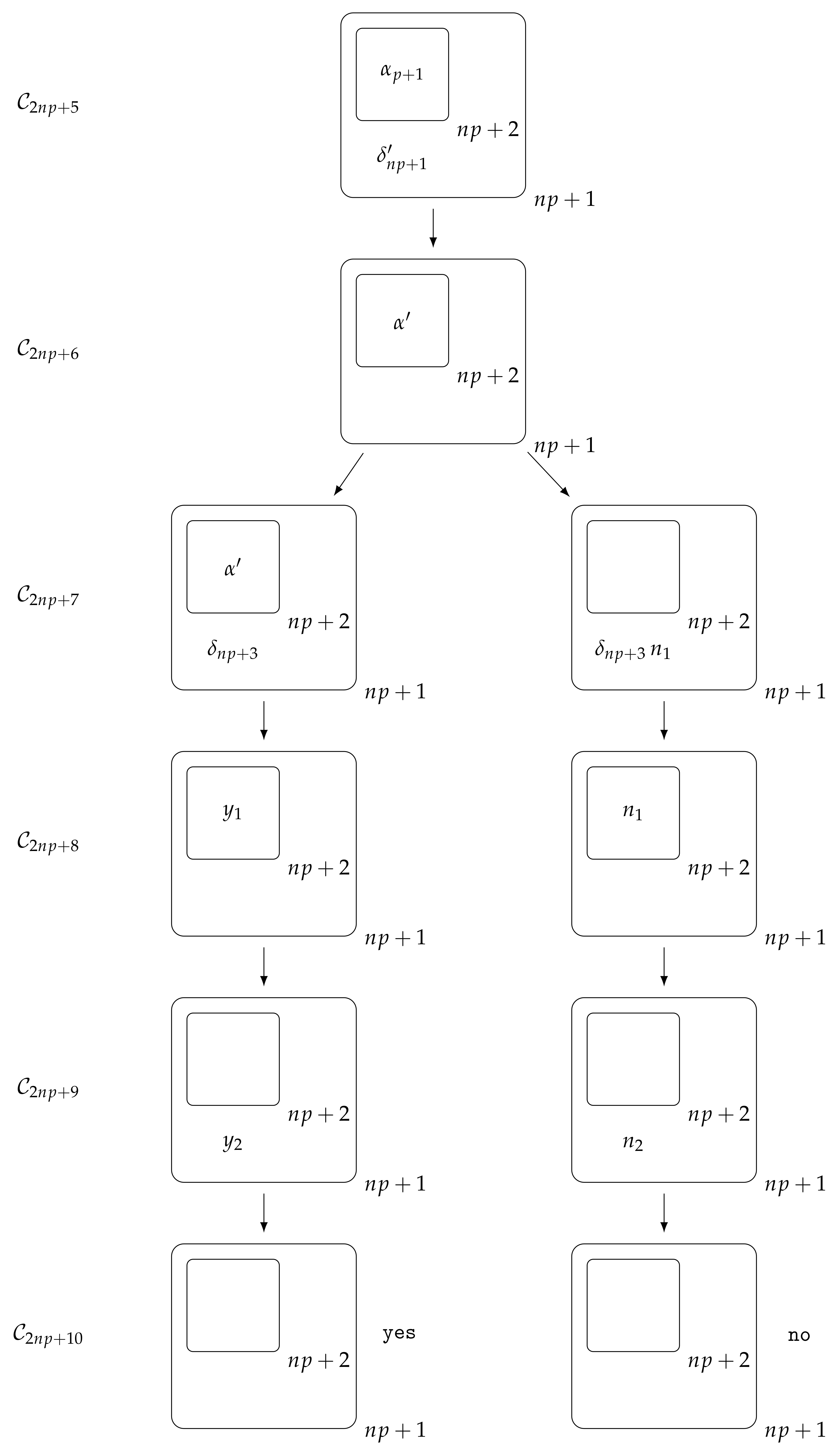
4.4. Output Stage

In configuration ${\mathcal{C}}_{2np+7}$, the existence of an object ${\alpha }^{\prime }$ in a membrane labelled by $np+2$ implies that no objects ${\alpha }_j$ remained in such a membrane; that is, that all clauses are satisfied by the corresponding truth assignment. Therefore, if there exists an object ${\alpha }^{\prime }$ in such a membrane, it implies that the formula $\phi$ is satisfiable. Thus, two different scenarios can be observed. On the one hand, if the formula is satisfiable, there exists at least one membrane labelled by $np+2$ at configuration ${\mathcal{C}}_{2np+7}$ such that it contains an object ${\alpha }^{\prime }$. In the next step, an object $y_1$ will be generated in such a membrane, that will be sent out, first to membrane $np+1$ as an object $y_2$, and finally to the environment as an object $\mathtt{yes}$. On the other hand, if the formula is unsatisfiable, no objects ${\alpha }^{\prime }$ remain in any of the membranes labelled by $np+2$ at configuration ${\mathcal{C}}_{2np+7}$. Objects $n_1$ will be sent to the membrane $np+1$ and, in the next step, they will be sent back to any membrane $np+2$, taking into account that the target membranes are selected in a non-deterministic way. In the next step, as the object ${\delta }_{np+3}$ still exists in membrane $np+1$, it reacts with an object $n_1$, transforming it into an object $n_2$ at the skin membrane, and in the last step of the configuration, it will be sent out to the environment as an object $\mathtt{no}$. It is important to take into account that, in the affirmative case, object ${\delta }_{np+3}$ is consumed, and since only one object of this kind exists, objects $n_1$ will not have any objects to react with. This stage takes exactly three computational steps, both in the affirmative case and in the negative case. In Figure 1, a graphical description of this process is provided to clarify how this stage works.

5. Results

The results of the paper will be discussed in this section.

Theorem 1.

$\mathtt{SAT}\in {\mathbf{PMC}}_{\mathcal{CDEC}\left(\right(2,1\left)\right)}$

Proof. 

The family of P systems constructed previously verifies the following:

• All the systems from $\mathbf{\Pi }=\{\Pi (n)\mid n\in \mathbb{N}\}$ are recognizer P systems from $\mathcal{CDEC}\left(\right(2,1\left)\right)$.
• The family $\mathbf{\Pi }$ is polynomially uniform by Turing machines given that, for each $n,p\in \mathbb{N}$, rules of $\Pi (\langle n,p\rangle )$ from $\mathbf{\Pi }$ are defined recursively by $n,p\in \mathbb{N}$, and the quantity of resources needed for constructing an element of the family is of polynomial order with respect to n and p, as it is shown below:

  –

  Alphabet size: $3n^2{p}^2+(11+\lfloor \frac{np}{2}\rfloor )np+2p+16\in \Theta \left(n^2{p}^2\right)$

  –

  Initial number of membranes: $np+5\in \Theta \left(np\right)$

  –

  Initial number of objects in cells: $np+p+4\in \Theta \left(np\right)$

  –

  Number of rules: $3n^2{p}^2\lfloor \frac{np}{2}\rfloor +2n{p}^2+15np+2p+16\in \Theta \left(n^3{p}^3\right)$

  –

  Maximum number of objects involved in a rule: $3\in \Theta \left(1\right)$.

• The pair of polynomial-time computable functions $(cod,s)$ defined complies the following: for each formula $\phi$ from $\mathtt{SAT}$, $s\left(\phi \right)$ is a natural number, $cod\left(\phi \right)$ is the input multiset of the system $\Pi \left(s\right(\phi \left)\right)$ and for each $t\in \mathbb{N}$, $s^{-1}\left(t\right)$ is a finite set.
• The family $\mathbf{\Pi }$ is polynomially bounded in time: in fact, for each formula $\phi$ from $\mathtt{SAT}$, the recognizer P system $\Pi \left(s\right(\phi \left)\right)+cod\left(\phi \right)$ takes exactly $2np+10$ computational steps in return an answer, either positive or negative, being n the number of variables and p the number of clauses of $\phi$.
• The family $\mathbf{\Pi }$ is sound with respect to $(X,cod,s)$: in fact, for each formula $\phi$, if the computations of $\Pi \left(s\right(\phi \left)\right)+cod\left(\phi \right)$ are accepting computations, then $\phi$ is satisfiable.
• The family $\mathbf{\Pi }$ is complete with respect to $(X,cod,s)$: in fact, for each formula $\phi$ that is satisfiable, all the computations of $\Pi \left(s\right(\phi \left)\right)+cod\left(\phi \right)$ are accepting computations.

□

Corollary 1.

$\mathbf{NP}\cup \mathbf{co}-\mathbf{NP}\subseteq {\mathbf{PMC}}_{\mathcal{CDEC}\left(\right(2,1\left)\right)}$

Proof. 

It is enough to observe that $\mathtt{SAT}$ is an NP-complete problem, $\mathtt{SAT}\in {\mathbf{PMC}}_{\mathcal{CDEC}\left(\right(2,1\left)\right)}$ and the class ${\mathbf{PMC}}_{\mathcal{CDEC}\left(\right(2,1\left)\right)}$ is closed under polynomial-time reduction and under complementary. □

In fact, this family does not use the environment with an active role, therefore:

Corollary 2.

$\mathbf{NP}\cup \mathbf{co}-\mathbf{NP}\subseteq {\mathbf{PMC}}_{\widehat{\mathcal{CDEC}}(2,1)}^{}$

Proof. 

It is enough to observe that $\mathbf{NP}\cup \mathbf{co}-\mathbf{NP}\subseteq {\mathbf{PMC}}_{\mathcal{CDEC}\left(\right(2,1\left)\right)}$ from the fact that a uniform family of recognizer membrane systems from $\mathcal{CDEC}\left(\right(2,1\left)\right)$ solving the problem $\mathtt{SAT}$ in polynomial time has been constructed, and this solution does use the environment only as the output of the system, $\mathcal{E}=\varnothing$, and does not take any object from it. □

Corollary 3.

$\mathbf{NP}\cup \mathbf{co}-\mathbf{NP}\subseteq {\mathbf{PMC}}_{\widehat{\mathcal{CDEC}}\left(3\right)}^{}$

6. Discussion

The idea of this solution is to use the power of division rules to generate all the possible truth assignments and objects first, and later on to use the parallel communication between membranes to transport all the needed objects. It is important to take into account that this is a great difference with P systems with active membranes, since in these systems, communication rules between membranes are limited to one object per membrane and time step. While the first stage takes the majority of the time, checking of the clauses and output of the system are executed in five time steps, using the created workspace in the generation stage. This implies that a great optimization (for instance, in the form of a parallel implementation) would be needed in order to generate the exponential number of membranes in polynomial (in this case, linear) time. In a practical way, this could lead to an interesting competitor with respect to the state-of-art $\mathtt{SAT}$ solvers, that are necessary to solve industrial propositional logic formulae used to improve some engineering processes.

7. Contributions

In this work, a solution to $\mathtt{SAT}$ by means of a family of recognizer membrane systems from $\widehat{\mathcal{CDEC}}(2,1)$ is given. In previous works, a similar result in the tissue-like counterpart was given, but using the environment as an active element. An interesting work would be to prove that the role of the environment is also irrelevant in tissue P systems with evolutional symport/antiport rules and division rules. Besides, similar results using separation rules instead of division rules were provided in the same work. Taking into account the differences between division rules and separation rules and between tissue-like and cell-like, it would be interesting to see if this result can also be translated to the cell-like framework. In this sense, a complete study of the role of the environment while using separation rules, both in the tissue-like and in the cell-like frameworks will be studied.

References

1. Păun, G. Computing with membranes. Turku Cent. Comput.-Sci.-Tucs Rep. 1998, 208, 108–143. [Google Scholar]
2. Martín-Vide, C.; Păun, G.; Pazos, J.; Rodríguez-Patón, A. Tissue P systems. Theor. Comput. Sci. 2003, 296, 295–326. [Google Scholar] [CrossRef] [Green Version]
3. Ionescu, M.; Păun, G.; Yokomori, T. Spiking neural P systems. Fundam. Inform. 2006, 71, 279–308. [Google Scholar]
4. Bao, T.; Yang, Q.; Peng, H.; Luo, X.; Wang, J. Computational power of sequential dendrite P systems. Theor. Comput. Sci. 2021, 893, 133–145. [Google Scholar] [CrossRef]
5. Wang, L.; Liu, X.; Zhao, Y. Universal Nonlinear Spiking Neural P Systems with Delays and Weights on Synapses. Comput. Intell. Neurosci. 2021, 2021, 3285719. [Google Scholar] [CrossRef]
6. Wu, T.; Pan, L.; Yu, Q.; Tan, K.C. Numerical Spiking Neural P Systems. IEEE Trans. Neural Netw. Learn. Syst. 2021, 32, 2443–2457. [Google Scholar] [CrossRef] [PubMed]
7. Păun, G. Membrane Computing: An Introduction, 1st ed.; Springer: Berlin/Heidelberg, Germany, 2002. [Google Scholar]
8. Păun, G.; Rozenberg, G.; Salomaa, A. The Oxford Handbook of Membrane Computing, 1st ed.; Oxford University Press, Inc.: New York, NY, USA, 2010. [Google Scholar]
9. Ciobanu, G.; Pérez-Jiménez, M.J.; Păun, G. Applications of Membrane Computing, 1st ed.; Springer: Berlin/Heidelberg, Germany, 2006. [Google Scholar]
10. Frisco, P.; Gheorghe, M.; Pérez-Jiménez, M.J. Applications of Membrane Computing in Systems and Synthetic Biology, 1st ed.; Springer International Publishing: Basel, Switzerland, 2014. [Google Scholar]
11. Zhang, G.; Pérez-Jiménez, M.J.; Gheorghe, M. Real-Life Applications with Membrane Computing, 1st ed.; Springer: Cham, Switzerland, 2017. [Google Scholar]
12. Zhang, G.; Pérez-Jiménez, M.J.; Riscos-Núñez, A.; Verlan, S.; Konur, S.; Hinze, T.; Gheorghe, M. Membrane Computing Models: Implementations, 1st ed.; Springer: Singapore, 2021. [Google Scholar]
13. Păun, G. Computing with membranes: Attacking NP-Complete Problems. In Proceedings of the Second International Conference on Unconventional Models of Computation, Brussels, Belgium, 13–16 December 2000; pp. 94–115. [Google Scholar]
14. Pérez-Jiménez, M.J.; Romero-Jiménez, Á.; Sancho-Caparrini, F. Complexity classes in models of cellular computing with membranes. Nat. Comput. 2003, 2, 265–285. [Google Scholar] [CrossRef]
15. Păun, G.; Pérez-Jiménez, M.J.; Riscos-Núñez, A. Tissue P Systems with Cell Division. In Proceedings of the Second Brainstorming Week on Membrane Computing, Sevilla, Spain, 2–7 February 2004; pp. 380–386. [Google Scholar]
16. Porreca, A.E.; Murphy, N.; Pérez-Jiménez, M.J. An optimal frontier of the efficiency of tissue P systems with cell division. In Proceedings of the Tenth Brainstorming Week on Membrane Computing, Sevilla, Spain, 30 January–3 February 2012; pp. 141–166. [Google Scholar]
17. Díaz-Pernil, D.; Pérez-Jiménez, M.J.; Romero-Jiménez, Á. Efficient simulation of tissue-like P systems by transition cell-like P systems. Nat. Comput. 2009, 8, 797–806. [Google Scholar] [CrossRef]
18. Pan, L.; Pérez-Jiménez, M.J.; Riscos-Núñez, A.; Rius, M. New frontiers of the efficiency in tissue P systems. In Proceedings of the Asian Conference on Membrane Computing (ACMC 2012), Wuhan, China, 15–18 October 2012; pp. 61–73. [Google Scholar]
19. Pérez-Jiménez, M.J.; Sosík, P. An Optimal Frontier of the Efficiency of Tissue P Systems with Cell Separation. Fundam. Inform. 2015, 138, 45–60. [Google Scholar] [CrossRef]
20. Macías-Ramos, L.F.; Pérez-Jiménez, M.J.; Riscos-Núñez, A.; Rius, M.; Valencia-Cabrera, L. The efficiency of tissue P systems with cell separation relies on the environment. In Proceedings of the Thirteenth International Conference on Membrane Computing (CMC 2012), Budapest, Hungary, 28–31 August 2013; pp. 277–290. [Google Scholar]
21. Pérez-Jiménez, M.J.; Riscos-Núñez, A.; Rius, M.; Romero-Campero, F.J. A polynomial alternative to unbounded environment for tissue P systems with cell division. Int. J. Comput. Math. 2013, 90, 760–775. [Google Scholar] [CrossRef]
22. Macías-Ramos, L.F.; Pérez-Jiménez, M.J.; Riscos-Núñez, A.; Valencia-Cabrera, L. Membrane fission versus cell division: When membrane proliferation is not enough. Theor. Comput. Sci. 2015, 608, 57–65. [Google Scholar] [CrossRef]
23. Macías-Ramos, L.F.; Song, B.; Song, T.; Pan, L.; Pérez-Jiménez, M.J. Limits on efficient computation in P systems with symport/antiport. In Proceedings of the Fifteenth Brainstorming Week on Membrane Computing, Sevilla, Spain, 31 January–3 February 2017; pp. 147–160. [Google Scholar]
24. Macías-Ramos, L.F.; Song, B.; Valencia-Cabrera, L.; Pan, L.; Pérez-Jiménez, M.J. Membrane fission: A computational complexity perspective. Complexity 2016, 21, 321–334. [Google Scholar] [CrossRef]
25. Orellana-Martín, D.; Valencia-Cabrera, L.; Riscos-Núñez, A.; Pérez-Jiménez, M.J. A path to computational efficiency through membrane computing. Theor. Comput. Sci. 2019, 777, 443–453. [Google Scholar] [CrossRef]
26. Orellana-Martín, D.; Valencia-Cabrera, L.; Song, B.; Pan, L.; Pérez-Jiménez, M.J. P systems with symport/antiport rules: When do the surroundings matter? Theor. Comput. Sci. 2020, 805, 206–217. [Google Scholar] [CrossRef]
27. Valencia-Cabrera, L.; Song, B.; Macías-Ramos, L.F.; Pan, L.; Riscos-Núñez, A.; Pérez-Jiménez, M.J. Minimal cooperation in P systems with symport/antiport: A complexity approach. In Proceedings of the Thirteenth Brainstorming Week on Membrane Computing, Sevilla, Spain, 2–6 February 2015; pp. 301–323. [Google Scholar]
28. Song, B.; Zhang, C.; Pan, L. Tissue-like P systems with evolutional symport/antiport rules. Inf. Sci. 2017, 378, 177–193. [Google Scholar] [CrossRef]
29. Orellana-Martín, D. The P vs NP Problem: Development of New Techniques through Bio-Inspired Models of Computation. Ph.D. Thesis, University of Sevilla, Sevilla, Spain, 2019. [Google Scholar]
30. Pan, L.; Song, B.; Valencia-Cabrera, L.; Pérez-Jiménez, M.J. The computational complexity of tissue P systems with evolutional symport/antiport rules. Complexity 2018, 3745210, 21. [Google Scholar] [CrossRef]
31. Orellana-Martín, D.; Valencia-Cabrera, L.; Song, B.; Pan, L.; Pérez-Jiménez, M.J. Narrowing frontiers with evolutional communication rules and cell separation. In Proceedings of the Sixteenth Brainstorming Week on Membrane Computing, Sevilla, Spain, 30 January–2 February 2018; pp. 123–162. [Google Scholar]
32. Orellana-Martín, D.; Valencia-Cabrera, L.; Song, B.; Pan, L.; Pérez-Jiménez, M.J. Tuning Frontiers of Efficiency in Tissue P systems with Evolutional Communication Rules. Complexity 2021, 2021, 7120840. [Google Scholar] [CrossRef]
33. Rozenberg, G.; Salomaa, A. Handbook of Formal Languages, 1st ed.; Springer: Berlin/Heidelberg, Germany, 1997. [Google Scholar]
Figure 1. Evolution of the final stage in the affirmative case (left) and in the negative case (right).
Axioms 10 00327 g001
Publisher’s Note: MDPI stays neutral with regard to jurisdictional claims in published maps and institutional affiliations.