Article

Global Stability Condition for the Disease-Free Equilibrium Point of Fractional Epidemiological Models †

by
Ricardo Almeida
,
Natália Martins
*,‡ and
Cristiana J. Silva
Center for Research and Development in Mathematics and Applications (CIDMA), Department of Mathematics, University of Aveiro, 3810-193 Aveiro, Portugal
*
Author to whom correspondence should be addressed.
Dedicated to Professor Delfim F. M. Torres on the occasion of his 50th birthday.
These authors contributed equally to this work.
Axioms 2021, 10(4), 238; https://doi.org/10.3390/axioms10040238
Submission received: 23 July 2021 / Revised: 15 September 2021 / Accepted: 17 September 2021 / Published: 25 September 2021

Abstract

:
In this paper, we present a new result that allows for studying the global stability of the disease-free equilibrium point when the basic reproduction number is less than 1, in the fractional calculus context. The method only involves basic linear algebra and can be easily applied to study global asymptotic stability. After proving some auxiliary lemmas involving the Mittag–Leffler function, we present the main result of the paper. Under some assumptions, we prove that the disease-free equilibrium point of a fractional differential system is globally asymptotically stable. We then exemplify the procedure with some epidemiological models: a fractional-order SEIR model with classical incidence function, a fractional-order SIRS model with a general incidence function, and a fractional-order model for HIV/AIDS.

1. Introduction

Fractional differential equations play an important role in modeling real-life phenomena. By replacing an integer-order derivative with a real-order fractional derivative, often we can fit the system of equations to the real data more efficiently because many dynamical systems cannot be completely described by ODEs. To mention a few of them, we refer applications to bioengineering [1,2], biology [3], Lévy motion [4], harmonic oscillators with damping [5], economy [6,7], and engineering [8,9]. In this work, we are particularly interested in applications of fractional calculus in epidemiological models. This topic has been intensively studied in the recent past, from the well formulation of the problem, the existence of equilibrium points, modeling, and forecasting of epidemiological systems. For example, Refs. [10,11,12] proposed fractional epidemiological models to study the spread of COVID-19 in different countries, Refs. [13,14] investigated the HIV infection, in Ref. [15], a varicella outbreak in China was considered, the spread of dengue fever outbreak in the Cape Verde islands was studied in [16], and in [17] a fractional measles model was proposed. Stability studies were given in e.g., [13,18,19,20,21] and numerical methods in e.g., [22,23,24]. We also refer to [25] where a review of several fractional epidemiological models was carried out.
An important problem is the study of the global stability of the equilibrium points, in order to better understand the evolution of the disease over time. That is, the system will evolve to the equilibrium point, independently of the starting points. The study of local stability is a relatively simple matter, as it usually involves finding the eigenvalues of the Jacobian matrix and studying their sign. However, the question of global stability is not, in many cases, simple to answer as it usually involves constructing suitable Lyapunov-like functions and there is no routine on how to find them. We emphasize here the fact that the use of the Lyapunov stability theory to establish the global asymptotic stability for fractional differential equations is more complicated than for the ODEs (see, e.g., [26,27,28,29]). This was the motivation to investigate a new method to study global asymptotic stability for dynamical systems described by fractional differential equations. In [30], a novel method was presented. By writing the system in a matricial form and analyzing the matrices involved is such procedure, under some simple assumptions, we can ensure that the equilibrium point is globally stable if the basic reproduction number R 0 is less than 1. The aim of this work is to generalize the main result of [30] to the fractional setting. To our knowledge, this is the first work on global stability following this last approach to the problem.
The paper is organized as follows. In Section 2, we present some concepts and known results needed for this work. Section 3 presents the new contributions of this paper. After deducing some auxiliary lemmas, we prove the main result of this work, Theorem 2. Under some assumptions that can be easily verified for a wide range of epidemiological models given by fractional differential systems, we prove that, if the basic reproduction number is less than 1, then the equilibrium point is globally asymptotically stable. Lastly, in Section 4, we present three examples to show the utility of our research.

2. Preliminaries

We begin this section with some basic definitions and results of the fractional calculus needed in this work. For more details, we refer the reader to [31,32].
Throughout the text, α ] 0 , 1 [ and Γ ( z ) = 0 t z 1 e t d t , z > 0 , is the Gamma function.
Definition 1.
Let f : R 0 + R be an integrable function. The (left-sided) Riemann–Liouville fractional integral of function f of order α is given by
I 0 + α f ( t ) : = 1 Γ ( α ) 0 t ( t τ ) α 1 f ( τ ) d τ , t > 0 .
Definition 2.
The (left-sided) Caputo fractional derivative of order α of function f C 1 ( R 0 + , R ) is defined by
C D 0 + α f ( t ) : = 1 Γ ( 1 α ) 0 t ( t τ ) α f ( τ ) d τ , t > 0 .
Next, we recall the definition of the generalized Mittag–Leffler function, which is a special function that generalizes the standard exponential function. The Mittag–Leffler function is of great importance in fractional calculus because it arises naturally in the solution of fractional-order differential and integral equations.
Definition 3.
The Mittag–Leffler function with two parameters is defined by
E α , β ( t ) : = k = 0 t k Γ ( α k + β ) , t C ,
with α , β 0 . When β = 1 , we define the one parameter Mittag–Leffler function E α ( t ) : = E α , 1 ( t ) .
To understand the theory of fractional differential equations, one needs to know properties of these special functions. Its main properties and applications can be found, for example, in [33]. We emphasize here the fact that E α , β ( t ) can take negative values (cf. [34]).
Recently, we have observed an increasing interest in the Mittag–Leffler function for matrix arguments, since the solution of many systems of differential equations of noninteger order can be expressed using this matrix function. For theoretical properties and a survey on numerical approximation of the matrix Mittag–Leffler function, we recommend the recent paper [35] and the references cited therein.
Definition 4.
Given A C n × n , the matrix Mittag–Leffler function with two parameters is defined through the convergent series
E α , β ( A ) : = k = 0 A k Γ ( α k + β )
where α , β 0 . If β = 1 , we define the one parameter matrix Mittag–Leffler function E α ( A ) : = E α , 1 ( A ) .
Remark 1.
For α = β = 1 , the matrix Mittag–Leffler function is the matrix exponential, that is, E 1 , 1 ( A ) = exp ( A ) = k = 0 A k k ! . Unfortunately, as noticed in [36], there are several works where some properties of the matrix exponential were incorrectly extended to the matrix Mittag–Leffler function and then used to solve certain linear matrix fractional differential equations. One of the properties that cannot be extended to the matrix Mittag–Leffler function is the semigroup property: for given commutating matrices A and B, in general, we have E α ( A + B ) E α ( A ) · E α ( B ) . We note, however, that, if matrices A and B commute and α 1 , then E α ( A + B ) E α ( A ) · E α ( B ) .
We recall now two properties of the matrix Mittag–Leffler function that are useful in the present work (see [35]):
  • if A = diag ( a 11 , , a n n ) , then E α , β ( A ) = diag ( E α , β ( a 11 ) , , E α , β ( a n n ) ) ;
  • if there exists a non-singular matrix P such that A = P D P 1 , then E α , β ( A ) = P E α , β ( D ) P 1 .
To finalize this section, we review some concepts on matrix theory.
Definition 5.
We say that a square matrix A is an M-matrix if the off-diagonal entries are nonpositive and the real parts of all eigenvalues are nonnegative.
Given a square matrix A, the set of eigenvalues of A is denoted by σ ( A ) . The spectral bound of matrix A is defined as m ( A ) = max { Re ( λ ) : λ σ ( A ) } , where Re ( λ ) denotes the real part of λ , and the spectral radius of A is defined as ρ ( A ) = max { | λ | : λ σ ( A ) } .
The following result is a fundamental tool in the proof of Lemma 4.
Lemma 1
([36]). Let A = a b c d be a diagonalizable matrix of order 2 with eigenvalues λ 1 = ( a + d ) Ω 2 and λ 2 = ( a + d ) + Ω 2 where Ω : = ( a d ) 2 + 4 b c . Let e 1 : = E α , β ( λ 1 ) and e 2 : = E α , β ( λ 2 ) . If Ω and c are not zero, the matrix Mittag–Leffler function of matrix A is
E α , β ( A ) = 1 2 Ω ( d a ) ( e 1 e 2 ) + Ω ( e 1 + e 2 ) 2 b ( e 1 e 2 ) 2 c ( e 1 e 2 ) ( d a ) ( e 1 e 2 ) + Ω ( e 1 + e 2 ) .
We remark that, in Lemma 1, if Ω = 0 or c = 0 , a simple formula for the Mittag–Leffler function of a diagonalizable matrix of order 2 can be easily obtained.
Theorem 1
(cf. [37]). Let A R n × n . If the spectrum of A satisfies the relation
σ ( A ) λ C { 0 } : | arg ( λ ) | > α π 2 ,
then lim t E α ( A t α ) = 0 .

3. Main Results

Suppose that the epidemiological model under study is described by the fractional differential system
C D 0 + α X ( t ) = F ( X , I ) C D 0 + α I ( t ) = G ( X , I ) G ( X , 0 ) = 0
with nonnegative initial conditions X ( 0 ) = X 0 R m and I ( 0 ) = I 0 R n , where the components of the vector X denote the number of uninfected individuals (e.g., susceptible, recovered, vaccinated, etc.) and the components of I denote the number of the infected and infectious (the ones that can transmit the disease, such as the asymptomatic but infectious and active infected). In addition, we assume that function F is continuous, G is of class C 1 , and the fractional differential system (1) with initial conditions X ( 0 ) = X 0 and I ( 0 ) = I 0 admits a unique solution.
Throughout this paper, we denote by U 0 = ( X , 0 ) R m + n the disease-free equilibrium (DFE) point of the system (1), that is, F ( X , 0 ) = G ( X , 0 ) = 0 .
Let A : = G I ( X , 0 ) and assume that matrix A can be written in the form A = M D , where M , D are two square matrices with M 0 (all entries are nonnegative), and D > 0 is a diagonal matrix. The following result was proven in [38]:
m ( A ) < 0 if   and   only   if ρ ( M D 1 ) < 1 ,
or
m ( A ) > 0 if   and   only   if ρ ( M D 1 ) > 1 .
The value
R 0 : = ρ ( M D 1 )
plays an important role in epidemiological models, and it is known as the basic reproduction number. This number gives the average number of secondary cases produced by one infected individual in a population where all individuals are susceptible to the infection.
The following result is well known in the literature. For the convenience of the reader, we present here one possible proof that follows from the fact that the scalar Mittag–Leffler function is completely monotonic ([39,40]).
Lemma 2.
For 0 < α < 1 , E α , α ( t ) 0 , for all t R .
Proof. 
Clearly, E α , α ( t ) 0 , for all t 0 . To prove that E α , α ( t ) 0 , for all t > 0 , we use the fact that the scalar Mittag–Leffler function E α ( t ) , t 0 , is completely monotonic, that is,
( 1 ) m d m d t m E α ( t ) 0 , m N .
Since
α d d t E α ( t ) = E α , α ( t ) , t 0 ,
it follows from (2) that
E α , α ( t ) 0 , t 0 .
This completes the proof. □
The following result is also useful in this work.
Lemma 3.
For 0 < α < 1 , E α , α : R R is an increasing function.
Proof. 
It is clear that E α , α is an increasing function on R 0 + . Now, we prove that d d t E α , α ( t ) 0 , for all t R 0 . Since
d d t E α , α ( t ) = α d 2 d t 2 E α ( t ) = k = 1 k t k 1 Γ ( k α + α ) ,
from (2), we conclude that d d t E α , α ( t ) 0 , proving the desired result. □
Now, we prove the following lemma that shows the applicability of our main result (Theorem 2).
Lemma 4.
Let A R 2 × 2 be a matrix and 0 < α < 1 . If matrix A is diagonalizable and A is an M-matrix, then E α , α ( A ) 0 .
Proof. 
With our assumptions and using the notations from Lemma 1, we have that b , c , Ω R 0 + , λ 1 , λ 2 R 0 , and λ 2 λ 1 . First, suppose that Ω 0 and c 0 . Hence, from Lemmas 2 and 3, we conclude that e 2 : = E α , α ( λ 2 ) e 1 : = E α , α ( λ 1 ) 0 . It remains to be proved that
Ω ( e 1 + e 2 ) ( d a ) ( e 1 e 2 ) and Ω ( e 1 + e 2 ) ( d a ) ( e 1 e 2 ) .
Suppose that d a (the other case is similar). Then, we just need to prove the first inequality. Since both sides of the inequality are nonnegative, we have that
[ ( a d ) 2 + 4 b c ] ( e 1 + e 2 ) 2 ( d a ) 2 ( e 1 e 2 ) 2 ,
which is equivalent to
( a d ) 2 e 1 2 + ( a d ) 2 e 2 2 + 2 ( a d ) 2 e 1 e 2 + 4 b c ( e 1 + e 2 ) 2 ( a d ) 2 e 1 2 + ( a d ) 2 e 2 2 2 ( a d ) 2 e 1 e 2
proving the desired. Now, we suppose that c = 0 and a d . If a < d , then we get
E α , β ( A ) = e 1 b a d ( e 1 e 2 ) 0 e 2 0 ,
and, if a > d , then
E α , β ( A ) = e 2 b a d ( e 2 e 1 ) 0 e 1 0 .
If c = 0 and a = d , then
E α , β ( A ) = e 1 0 0 e 1 0
since b = 0 (otherwise, A is not diagonalizable). If Ω = 0 , the proof is trivial since in this case A is diagonalizable iff a = d and c = d = 0 . □
The following result is a fundamental tool in the proof of Theorem 2.
Lemma 5.
Let B R n × n be an invertible matrix and H : R m + n R n be a continuous function. Suppose that the fractional differential equation
C D 0 + α I ( t ) = B · I ( t ) H ( X ( t ) , I ( t ) )
with initial condition I ( 0 ) = I 0 R n , has a unique solution. Then, the solution of this initial value problem satisfies
I ( t ) = E α ( B t α ) · I 0 0 t B 1 · d d s E α ( B s α ) · H ( X ( t s ) , I ( t s ) ) d s .
Proof. 
The proof follows the ideas from [41] (Theorem 7.2). First, observe that
C D 0 + α ( E α ( B t α ) · I 0 ) = B · E α ( B t α ) · I 0 .
To compute
C D 0 + α 0 t B 1 · d d s E α ( B s α ) · H ( X ( t s ) , I ( t s ) ) d s ,
let
y ¯ ( t ) = 0 t B 1 · d d s E α ( B s α ) · H ( X ( t s ) , I ( t s ) ) d s .
Since
B 1 · d d s E α ( B s α ) = α s α 1 E α ( B s α ) = α s α 1 k = 1 k ( B s α ) k 1 Γ ( k α + 1 ) = k = 1 B k 1 s α k 1 Γ ( k α ) ,
we get the following:
y ¯ ( t ) = k = 1 B k 1 Γ ( k α ) 0 t s α k 1 H ( X ( t s ) , I ( t s ) ) d s = k = 1 B k 1 Γ ( k α ) 0 t ( t τ ) α k 1 H ( X ( τ ) , I ( τ ) ) d τ = k = 1 B k 1 · I 0 + α k H ( X ( t ) , I ( t ) ) .
Thus,
C D 0 + α y ¯ ( t ) = k = 1 B k 1 · C D 0 + α I 0 + α k H ( X ( t ) , I ( t ) ) = k = 1 B k 1 · I 0 + α ( k 1 ) H ( X ( t ) , I ( t ) ) = k = 0 B k · I 0 + α k H ( X ( t ) , I ( t ) ) = H ( X ( t ) , I ( t ) ) + k = 1 B k · I 0 + α k H ( X ( t ) , I ( t ) ) = H ( X ( t ) , I ( t ) ) + B · y ¯ ( t ) .
Hence, we may conclude that
C D 0 + α I ( t ) = B · E α ( B t α ) · I 0 H ( X ( t ) , I ( t ) ) B · y ¯ ( t ) = B · E α ( B t α ) · I 0 y ¯ ( t ) H ( X ( t ) , I ( t ) ) = B · I ( t ) H ( X ( t ) , I ( t ) ) ,
proving the desired result. □
We are now in conditions to present a new global stability condition for the DFE of system (1) when R 0 < 1 . Knowing that an equilibrium point is globally asymptotically stable with respect to the system that describes the evolution of the uninfected individuals, and with some extra assumptions related to the matrices involved in the system associated with infected and infectious individuals, we can conclude that the equilibrium point is in fact globally asymptotically stable with respect to the complete system. Although the result imposes some restrictions in order to be applied, for many epidemiological models, it can be easily used, as we will illustrate in Section 4.
Theorem 2.
Suppose that
1.
For C D 0 + α X ( t ) = F ( X , 0 ) , the vector X is globally asymptotically stable;
2.
Function G can be written as G ( X , I ) = A · I G ^ ( X , I ) , where G ^ ( X , I ) 0 for all ( X , I ) , and A = G I ( X , 0 ) can be written as A = M D , where M 0 and D > 0 is a diagonal matrix;
3.
Matrix A is diagonalizable, the real parts of the eigenvalues of A are nonpositive, and E α , α ( A ) 0 ;
4.
I ( t ) 0 for all t > 0 (nonnegativity of solutions).
If R 0 < 1 , then the DFE, U 0 = ( X , 0 ) , is a globally asymptotically stable equilibrium of system (1), for all 0 < α < 1 .
Proof. 
First, observe that, since R 0 < 1 , then m ( A ) < 0 (see [38]), and so matrix A is invertible. Since
C D 0 + α I ( t ) = G ( X ( t ) , I ( t ) ) = A · I ( t ) G ^ ( X ( t ) , I ( t ) ) ,
then, by Lemma 5, we get
0 I ( t ) = E α ( A t α ) · I 0 0 t A 1 d d s E α ( A s α ) · G ^ ( X ( t s ) , I ( t s ) ) d s E α ( A t α ) · I 0 ,
since
A 1 d d s E α ( A s α ) = α s α 1 E α ( A s α ) = s α 1 E α , α ( A s α ) 0 .
Since the real parts of the eigenvalues of matrix A are negative, from Theorem 1, we get
lim t E α ( A t α ) = 0 ,
and hence
lim t I ( t ) = 0 .
Since X is globally asymptotically stable with respect to C D 0 + α X ( t ) = F ( X , 0 ) , which in turn is the limiting system of C D 0 + α X ( t ) = F ( X , I ) , then we get
lim t X ( t ) = X ( t ) ,
which completes the proof. □
Remark 2.
Note that the assumption E α , α ( A ) 0 in Theorem 2 is trivially satisfied if matrix A has dimensions 1 or 2 (by Lemmas 2 and 4, respectively). In addition, if α 1 , since E α , α ( A ) exp ( A ) , the above condition also holds for any matrix A R n × n .

4. Examples

In this section, we illustrate our main result, Theorem 2, by considering three Caputo fractional-order compartmental models and show that the disease free equilibrium is globally stable in all the cases, whenever R 0 < 1 . We stress that usually (see e.g., [21]) the global stability of the disease free equilibrium is proved by considering an appropriate Lyapunov function and LaSalle’s invariance principle [42], which are often difficult to apply especially when the model has a considerable number of variables and parameters. Our main result allows us to prove the global stability of the disease free equilibrium in an easier and simpler way. For the numerical implementation of the fractional derivatives, we have used the Adams–Bashforth–Moulton scheme, which has been implemented in the Matlab code fde12 by Garrappa [43].
The code implements the predictor–corrector PECE method of Adams–Bashforth–Moulton type described in [44]. We fixed a time step size of h = 2 6 and consider, without loss of generality, the fractional-order derivatives α { 0.8 , 0.85 , 0.9 , 0.95 , 1.0 } .

4.1. A Fractional SEIR Model with Traditional Incidence Rate

We start by considering a Caputo fractional-order version of the classical SEIR model that has been applied to describe the transmission dynamics of infectious diseases where there exists a significant latency period during which the individuals are infected but not yet infectious. During this period, the individual is in the so-called exposed compartment E, see e.g., [45]. The other compartments of the model are susceptible S, infected I, and recovered R, and each of them denotes a fraction of the total population. The following assumptions are considered: the birth and death rates are assumed to be equal, and denoted by μ ; the incidence rate is the traditional one, given by β S I , where β represents the transmission rate; the latent period is denoted by ε ; infected individuals recover at a rate γ and remain recovered with permanent immunity. All parameters are assumed to be positive. The model is given by the following system:
C D 0 + α S ( t ) = μ μ S ( t ) β S ( t ) I ( t ) , C D 0 + α E ( t ) = ( ε + μ ) E ( t ) + β S ( t ) I ( t ) , C D 0 + α I ( t ) = ε E ( t ) ( γ + μ ) I ( t ) , C D 0 + α R ( t ) = γ I ( t ) μ R ( t ) .
The disease-free equilibrium of the model (3) is given by
Σ 0 = S 0 , E 0 , I 0 , R 0 = 1 , 0 , 0 , 0 .
Following the notation from Section 3, we have
A = ε μ β ε γ μ .
The matrix A can be written as A = M D with
M = 0 β ε 0
and
D = ε + μ 0 0 γ + μ .
The point X = ( 1 , 0 ) is globally asymptotically stable for the system of uninfected individuals:
C D 0 + α S ( t ) = μ μ S ( t ) , C D 0 + α R ( t ) = μ R ( t ) .
It is easy to verify that the function
R ( t ) = R 0 E α μ t α
satisfies the second equation of (4). From [41] (Theorem 7.2), the solution of the first equation of (4) is the function
S ( t ) = S 0 E α μ t α + 0 t μ s α 1 E α , α μ s α d s .
Simple computations lead to
S ( t ) = S 0 E α μ t α E α μ t α + 1 .
Thus,
( S ( t ) , R ( t ) ) ( 1 , 0 ) a s t .
In addition, by Lemma 4, E α , α ( A ) is nonnegative and so, by Theorem 2, the disease-free equilibrium of the model (9) is globally asymptotically stable.
Consider the following parameter values: μ = 1 / 80 , β = 0.05 and γ = 1 , ε = 1 . Then, the eigenvalues of the matrix A are 0.7888 and 1.2361 ; therefore, m ( A ) < 0 . Moreover, we confirm that R 0 : = ρ ( M D 1 ) = 0.2893 < 1 .
Through adequate numerical simulations, we illustrate the global stability of the disease free equilibrium, whenever R 0 < 1 , considering different values of α and initial conditions. In Figure 1, we consider different values for α and the initial condition x 0 from (5).
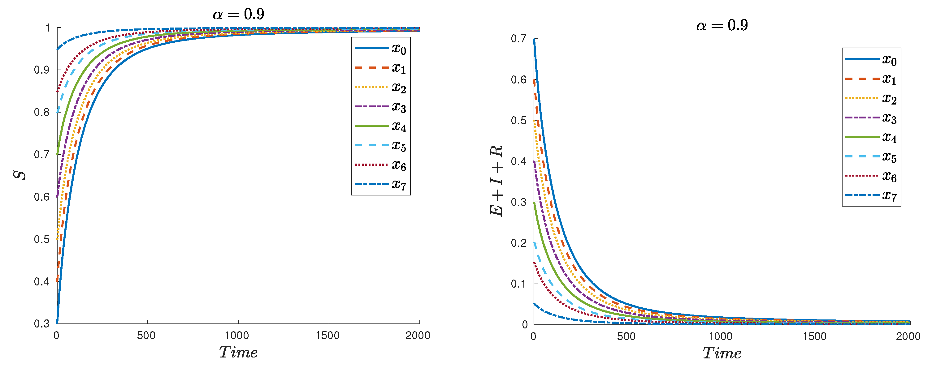
The global stability of the disease free equilibrium Σ 0 = ( 1 , 0 , 0 , 0 ) is illustrated in Figure 2, considering different initial conditions x i , i = 0 , , 7 , given by (5):
x 0 = S 0 , 0 , E 0 , 0 , I 0 , 0 , R 0 , 0 = ( 0.3 , 0.5 , 0.1 , 0.1 ) , x 1 = S 0 , 1 , E 0 , 1 , I 0 , 1 , R 0 , 1 = ( 0.4 , 0.1 , 0.3 , 0.2 ) , x 2 = S 0 , 2 , E 0 , 2 , I 0 , 2 , R 0 , 2 = ( 0.5 , 0.05 , 0.4 , 0.05 ) , x 3 = S 0 , 3 , E 0 , 3 , I 0 , 3 , R 0 , 3 = ( 0.6 , 0.1 , 0.2 , 0.1 ) , x 4 = S 0 , 4 , E 0 , 4 , I 0 , 4 , R 0 , 4 = ( 0.7 , 0.05 , 0.1 , 0.15 ) , x 5 = S 0 , 5 , E 0 , 5 , I 0 , 5 , R 0 , 5 = ( 0.8 , 0.1 , 0.1 , 0.0 ) , x 6 = S 0 , 6 , E 0 , 6 , I 0 , 6 , R 0 , 6 = ( 0.85 , 0.05 , 0.1 , 0.0 ) , x 7 = S 0 , 7 , E 0 , 7 , I 0 , 7 , R 0 , 7 = ( 0.95 , 0.025 , 0.025 , 0.0 ) .

4.2. A Fractional SIRS Model with General Incidence Rate

In the second example, we consider the Caputo fractional-order version of the classical S I R S model from [21], given by the following system:
C D 0 + α S ( t ) = Λ μ S ( t ) β I ( t ) S ( t ) 1 + k 1 S ( t ) + k 2 I ( t ) + k 3 S ( t ) I ( t ) + λ R ( t ) , C D 0 + α I ( t ) = β I ( t ) S ( t ) 1 + k 1 S ( t ) + k 2 I ( t ) + k 3 S ( t ) I ( t ) ( μ + r ) I ( t ) , C D 0 + α R ( t ) = r I ( t ) ( μ + λ ) R ( t ) .
The model considers a homogeneous population divided into three subgroups: susceptible individuals S ( t ) , infected and infectious individuals I ( t ) , and recovered R ( t ) , individuals at time t. The parameters Λ , β , μ , and r, represent the recruitment rate of the population, the infection rate, the natural death rate, and the recovery rate of the infected individuals, respectively. The rate that recovered individuals lose immunity and return to the susceptible class is represented by λ . While contacting with infected individuals, the susceptible become infected at the incidence rate
β S I 1 + k 1 S + k 2 I + k 3 S I ,
where k 1 , k 2 , and k 3 are nonnegative constants [21]. We remark that system (6) admits a unique positive solution (see [21] (Theorem 7)).
The disease-free equilibrium of the model (6) is given by
Σ 0 = S 0 , I 0 , R 0 = Λ μ , 0 , 0 .
In this case, following the notation from Section 3,
A = M D = Λ β Λ k 1 + μ μ r
with
M = Λ β Λ k 1 + μ and D = [ μ + r ] .
Hence,
R 0 = ρ ( M D 1 ) = Λ β ( μ + r ) ( Λ k 1 + μ ) .
We easily conclude that A < 0 whenever R 0 < 1 .
In what follows, we prove that the first condition of Theorem 2 holds, that is, X = ( Λ / μ , 0 ) is globally asymptotically stable for the system of uninfected individuals:
C D 0 + α S ( t ) = Λ μ S ( t ) + λ R ( t ) , C D 0 + α R ( t ) = ( μ + λ ) R ( t ) .
The solution of the fractional differential equations (7) is the functions
R ( t ) = R 0 E α ( μ + λ ) t α
and
S ( t ) = S 0 E α μ t α + 0 t Λ + λ R 0 E α ( μ + λ ) ( t s ) α s α 1 E α , α μ s α d s .
Obviously R ( t ) 0 , as t goes to infinity. Now, we prove that S ( t ) Λ / μ , as t . First, observe that
0 t s α 1 E α , α μ s α d s = k = 0 ( μ ) k Γ ( k α + α ) 0 t s k α + α 1 d s = k = 0 ( μ ) k Γ ( k α + α + 1 ) t k α + α = 1 μ k = 0 ( μ ) k + 1 Γ ( ( k + 1 ) α + 1 ) t ( k + 1 ) α = 1 μ E α μ t α 1 .
For the other term inside the integral, we get
0 t E α ( μ + λ ) ( t s ) α s α 1 E α , α μ s α d s = m = 0 k = 0 ( ( μ + λ ) ) m ( μ ) k Γ ( m α + 1 ) Γ ( k α + α ) 0 t ( t s ) m α s k α + α 1 d s .
To evaluate this integral, we use the known formula involving the Beta function:
B ( x , y ) = Γ ( x ) Γ ( y ) Γ ( x + y ) , x , y > 0 .
With the change of variable u = s / t , we get
0 t ( t s ) m α s k α + α 1 d s = t m α 0 t ( 1 s / t ) m α s k α + α 1 d s = t m α + k α + α 0 1 ( 1 u ) m α u k α + α 1 d u = t m α + k α + α B ( k α + α , m α + 1 ) = t m α + k α + α Γ ( k α + α ) Γ ( m α + 1 ) Γ ( m α + k α + α + 1 ) .
Thus, we prove that the solution S ( · ) is given by
S ( t ) = S 0 E α μ t α + Λ μ 1 E α μ t α + λ R 0 m = 0 k = 0 ( ( μ + λ ) ) m ( μ ) k Γ ( m α + k α + α + 1 ) t m α + k α + α .
Observe that, as t goes to infinity,
S 0 E α μ t α 0 and Λ μ 1 E α μ t α Λ μ .
To sum up, it remains to prove that the double sum converges to zero. For that purpose, we recall the concept of the Mittag–Leffler function of two variables (cf. [46]) E α , β ( x , y , · ) . With such notation, we can write
m = 0 k = 0 ( ( μ + λ ) ) m ( μ ) k Γ ( m α + k α + α + 1 ) t m α + k α + α = t α E α , α ( ( μ + λ ) t α , μ t α , α + 1 )
which converges to zero, as t goes to infinity, by [46] (Theorem 3.1). This proves the desired conclusion. We also remark that, by Lemma 2, E α , α ( A ) is nonnegative. Therefore, by Theorem 2, the disease-free equilibrium of the model (6) is globally asymptotically stable.
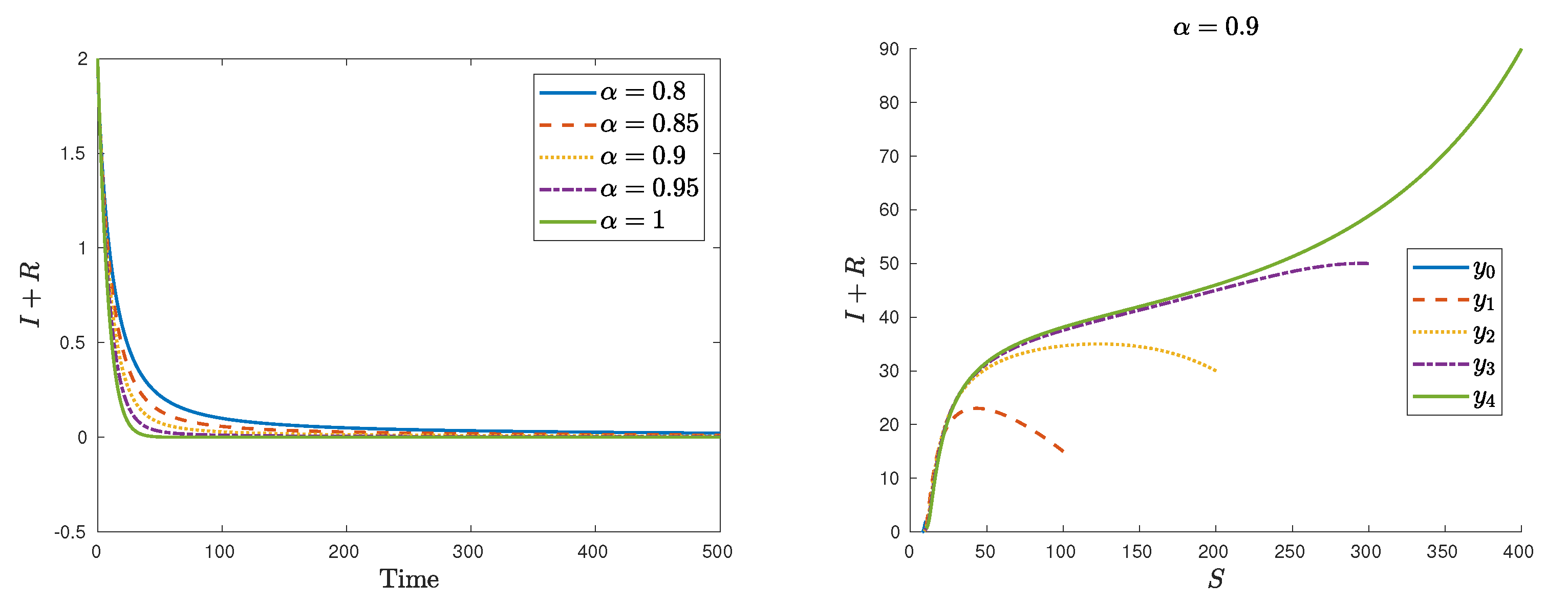
Considering the parameter values from [21], Λ = 0.8 , μ = 0.1 , λ = 0.5 , β = 0.1 , r = 0.5 , k 1 = 0.1 , k 2 = 0.02 , and k 3 = 0.003 , we have R 0 = 0.7407 < 1 . For initial conditions, we consider the following ones and without any specific criteria:
y 0 = S 0 , 0 , I 0 , 0 , R 0 , 0 = ( 10 , 1 , 1 ) , y 1 = S 0 , 1 , I 0 , 1 , R 0 , 1 = ( 100 , 10 , 5 ) , y 2 = S 0 , 2 , I 0 , 2 , R 0 , 2 = ( 200 , 20 , 10 ) , y 3 = S 0 , 3 , I 0 , 3 , R 0 , 3 = ( 300 , 30 , 20 ) , y 4 = S 0 , 4 , I 0 , 4 , C 0 , 4 , A 0 , 5 = ( 400 , 40 , 50 ) .
The stability of the disease free equilibrium for model (6) is illustrated in Figure 3.

4.3. A Modified Fractional SICA Model for HIV/AIDS

In this example, we consider a modified Caputo fractional-order model for HIV/AIDS, based on the model proposed in [14,47]. We show that this fractional model satisfies the conditions of Theorem 2 and, through some numerical simulations, we illustrate the global stability of the disease free equilibrium, when R 0 < 1 .
In this model, the total population is assumed to be homogeneous and divided into four mutually-exclusive compartments: susceptible individuals (S); HIV-infected individuals with no clinical symptoms of AIDS but able to transmit HIV to other individuals (I); HIV-infected individuals under antiretroviral (ART) treatment (the so called chronic stage) with a viral load remaining low (C); and HIV-infected individuals with AIDS clinical symptoms (A). Analogously to the assumption made in [47], we consider that individuals in the chronic stage C have a very low viral load and do not transmit HIV infection [48], but, differently from [47], we assume that individuals with AIDS A, due to their higher viral load, may transmit HIV virus, at a rate η A β with η A > 1 . Therefore, effective contact with people infected with HIV is at a rate λ , given by
λ = β I + η A A ,
where β is the effective contact rate for HIV transmission. We assume that the recruitment rate is equal to the natural death rate and is denoted by μ . The following assumptions are the same as in [14]. HIV-infected individuals with no AIDS symptoms I progress to the class of individuals with HIV infection under ART treatment C, at a rate ϕ , and HIV-infected individuals with AIDS symptoms are treated for HIV at rate γ . Individuals in the class C leave for the class I, at a rate ω . HIV-infected individuals with AIDS symptoms A that start treatment move to the class of HIV-infected individuals I, moving to the chronic class C only if the treatment is maintained. HIV-infected individuals with no AIDS symptoms I that do not take ART treatment progress to the AIDS class A, at rate ρ . Only HIV-infected individuals with AIDS symptoms A suffer from an AIDS induced death, at a rate d. The total population at time t, denoted by N ( t ) , is given by N ( t ) = S ( t ) + I ( t ) + C ( t ) + A ( t ) . The Caputo fractional-order system that describes the previous assumptions is given by
C D 0 + α S ( t ) = μ β I ( t ) + η A A ( t ) S ( t ) μ S ( t ) , C D 0 + α I ( t ) = β I ( t ) + η A A ( t ) S ( t ) ( ρ + ϕ + μ ) I ( t ) + ω C ( t ) + γ A ( t ) , C D 0 + α C ( t ) = ϕ I ( t ) ( ω + μ ) C ( t ) , C D 0 + α A ( t ) = ρ I ( t ) ( γ + μ + d ) A ( t ) .
The disease free equilibrium of system (9) is given by
Σ 0 = S 0 , I 0 , C 0 , A 0 = 1 , 0 , 0 , 0 .
Using the notation from Section 3, we have
A = β ρ ϕ μ β η A + γ ρ γ μ d .
The matrix A can be written as A = M D with
M = β β η A + γ ρ 0
and
D = ρ + ϕ + μ 0 0 γ + μ + d .
In this case, we will prove that X = ( 1 , 0 ) is globally asymptotically stable for the system of uninfected individuals:
C D 0 + α S ( t ) = μ μ S ( t ) , C D 0 + α C ( t ) = ( ω + μ ) C ( t ) .
The solution of (11) is
C ( t ) = C 0 E α ( ω + μ ) t α
and
S ( t ) = S 0 E α μ t α + 0 t μ s α 1 E α , α μ s α d s .
Similarly to Example Section 4.1, we can prove that the disease-free equilibrium of the model (9) is globally asymptotically stable.
Let us consider the parameter values from Table 1.
Then, the eigenvalues of the matrix A are 0.9612 and 1.4474 ; therefore, m ( A ) < 0 . Moreover, we confirm that R 0 : = ρ ( M D 1 ) = 0.1863 < 1 .
We now show, using numerical simulations, that for different values of α and initial conditions, the global stability of the disease free equilibrium holds, whenever R 0 < 1 .
In Figure 4, we consider different values for α and the initial conditions x 0 from (12).
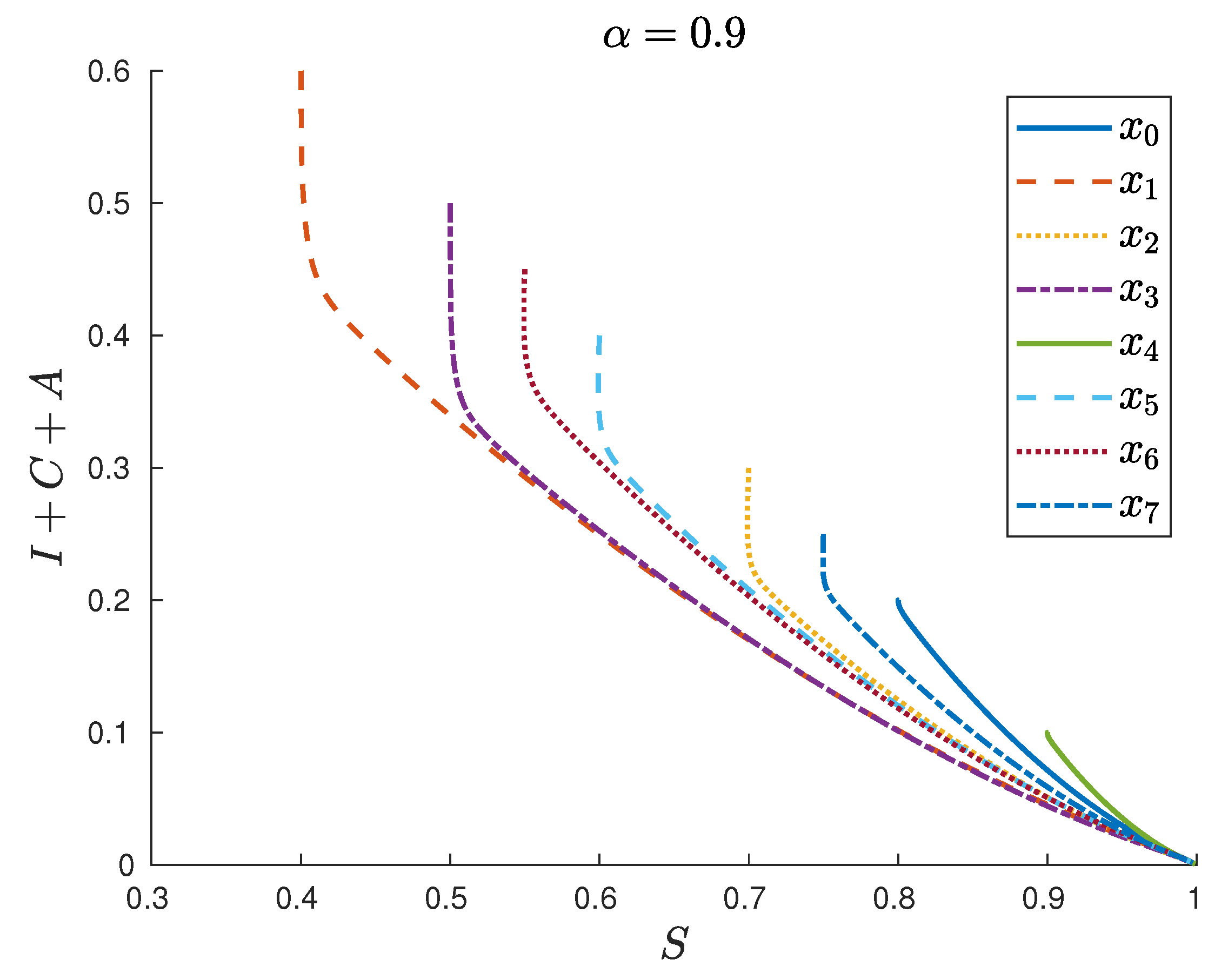
The global stability of the disease free equilibrium (10) is illustrated in Figure 5, considering different initial conditions x i , i = 0 , , 7 , given by (12).
x 0 = S 0 , 0 , I 0 , 0 , C 0 , 0 , A 0 , 0 = ( 0.8 , 0.1 , 0.1 , 0 ) , x 1 = S 0 , 1 , I 0 , 1 , C 0 , 1 , A 0 , 1 = ( 0.4 , 0.2 , 0.2 , 0.2 ) , x 2 = S 0 , 2 , I 0 , 2 , C 0 , 2 , A 0 , 2 = ( 0.7 , 0.1 , 0.1 , 0.1 ) , x 3 = S 0 , 3 , I 0 , 3 , C 0 , 3 , A 0 , 3 = ( 0.5 , 0.1 , 0.2 , 0.2 ) , x 4 = S 0 , 4 , I 0 , 4 , C 0 , 4 , A 0 , 4 = ( 0.9 , 0.05 , 0.05 , 0 ) , x 5 = S 0 , 5 , I 0 , 5 , C 0 , 5 , A 0 , 5 = ( 0.6 , 0.2 , 0.1 , 0.1 ) , x 6 = S 0 , 6 , I 0 , 6 , C 0 , 6 , A 0 , 6 = ( 0.55 , 0.25 , 0.1 , 0.1 ) , x 7 = S 0 , 7 , I 0 , 7 , C 0 , 7 , A 0 , 7 = ( 0.75 , 0.1 , 0.1 , 0.05 ) .

5. Conclusions

A new and simple result for the global stability for the disease-free equilibrium of fractional epidemiological models is presented. We highlight here the fact that the approach available in the literature so far involves the determination of an appropriate Lyapunov function, very laborious computations and, in the end, the application of LaSalle’s invariance principle. Our new method uses only basic results from matrix theory and some well-known results from fractional-order differential equations.
We also remark that the applicability of our main result, Theorem 2, is only possible if the matrix A satisfies the condition E α , α ( A ) 0 . We proved that, under the assumptions of Theorem 2, this condition holds if matrix A has dimensions 1 or 2. It would be interesting to check under what conditions we can guarantee that E α , α ( A ) 0 if the matrix A has dimensions greater than 2. Since many epidemiological models divide the population into subpopulations of epidemiological significance where the number of the infectious compartments are at most 2, our main result can be applied to a wide variety of epidemiological models.

Author Contributions

Conceptualization, R.A., N.M., and C.J.S.; methodology, R.A., N.M., and C.J.S.; formal analysis, R.A., N.M., and C.J.S.; writing—original draft preparation, R.A., N.M., and C.J.S.; writing—review and editing, R.A., N.M., and C.J.S. All authors have read and agreed to the published version of the manuscript.

Funding

Work is supported by Portuguese funds through the CIDMA-Center for Research and Development in Mathematics and Applications, and the Portuguese Foundation for Science and Technology (FCT-Fundação para a Ciência e a Tecnologia), within project UIDB/04106/2020. Cristiana J. Silva is also supported by FCT via the FCT Researcher Program CEEC Individual 2018 with reference CEECIND/00564/2018.

Institutional Review Board Statement

Not applicable.

Informed Consent Statement

Not applicable.

Data Availability Statement

Not applicable.

Acknowledgments

The authors are grateful to the two reviewer’s valuable comments that improved the manuscript.

Conflicts of Interest

The authors declare no conflict of interest.

References

  1. Ionescu, C.; Lopes, A.; Copot, D.; Machado, J.A.T.; Bates, J.H.T. The role of fractional calculus in modeling biological phenomena: A review. Commun. Nonlinear Sci. Numer. Simul. 2017, 51, 141–159. [Google Scholar] [CrossRef]
  2. Jesus, I.S.; Machado, J.A.T.; Cunha, J.B. Fractional electrical impedances in botanical elements. J. Vib. Control 2008, 14, 1389–1402. [Google Scholar] [CrossRef] [Green Version]
  3. Boukhouima, A.; Hattaf, K.; Lotfi, E.M.; Mahrouf, M.; Torres, D.F.M.; Yousfi, N. Lyapunov functions for fractional-order systems in biology: Methods and applications. Chaos Solitons Fractals 2020, 140, 110224. [Google Scholar] [CrossRef]
  4. Benson, D.A.; Wheatcraft, S.W.; Meerschaert, M.M. The fractional-order governing equation of Lévy motion. Water Resour. Res. 2000, 36, 1413–1423. [Google Scholar] [CrossRef]
  5. Stanislavsky, A.A. Fractional oscillator. Phys. Rev. E 2004, 70, 051103. [Google Scholar] [CrossRef] [Green Version]
  6. Skovranek, T. The Mittag–Leffler fitting of the Phillips curve. Mathematics 2019, 7, 589. [Google Scholar] [CrossRef] [Green Version]
  7. Xie, Y.; Wang, Z.; Meng, B. Stability and bifurcation of a delayed time-fractional order business cycle model with a general liquidity preference function and investment function. Mathematics 2019, 7, 846. [Google Scholar] [CrossRef] [Green Version]
  8. Maalej, B.; Khlif, R.J.; Mhiri, C.; Elleuch, M.H.; Derbel, N. Adaptive fractional control optimized by genetic algorithms with application to polyarticulated robotic systems. Math. Probl. Eng. 2021, 2021, 5579541. [Google Scholar] [CrossRef]
  9. Paola, M.; Pinnola, F.P.; Zingales, M. Fractional differential equations and related exact mechanical models. Comput. Math. Appl. 2013, 66, 608–620. [Google Scholar] [CrossRef] [Green Version]
  10. Barros, L.C.; Lopes, M.M.; Pedro, F.S.; Esmi, E.; Santos, J.P.C.; Sánchez, D.E. The memory effect on fractional calculus: An application in the spread of COVID-19. Comput. Appl. Math. 2021, 40, 72. [Google Scholar] [CrossRef]
  11. Bushnaq, S.; Saeed, T.; Torres, D.F.M.; Zeb, A. Control of COVID-19 dynamics through a fractional-order model. Alex. Eng. J. 2021, 60, 3587–3592. [Google Scholar] [CrossRef]
  12. Ndaïrou, F.; Area, I.; Nieto, J.J.; Silva, C.J.; Torres, D.F.M. Fractional model of COVID-19 applied to Galicia, Spain and Portugal. Chaos Solitons Fractals 2021, 144, 110652. [Google Scholar] [CrossRef] [PubMed]
  13. Liu, Z.; Lu, P. Stability analysis for HIV infection of CD4+ T-cells by a fractional differential time-delay model with cure rate. Adv. Differ. Equ. 2014, 2014, 298. [Google Scholar] [CrossRef]
  14. Silva, C.J.; Torres, D.F.M. Stability of a fractional HIV/AIDS model. Math. Comput. Simul. 2019, 164, 180–190. [Google Scholar] [CrossRef] [Green Version]
  15. Almeida, R.; Cruz, A.M.C.B.; Martins, N.; Monteiro, M.T.T. An epidemiological MSEIR model described by the Caputo fractional derivative. Int. J. Dyn. Control 2019, 7, 776–784. [Google Scholar] [CrossRef] [Green Version]
  16. Diethelm, K. A fractional calculus based model for the simulation of an outbreak of dengue fever. Nonlinear Dyn. 2013, 71, 613–619. [Google Scholar] [CrossRef]
  17. Qureshi, S.; Jan, R. Modeling of measles epidemic with optimized fractional order under Caputo differential operator. Chaos Solitons Fractals 2021, 145, 110766. [Google Scholar] [CrossRef]
  18. Goufo, E.F.D.; Maritz, R.; Munganga, J. Some properties of the Kermack-McKendrick epidemic model with fractional derivative and nonlinear incidence. Adv. Differ. Equ. 2014, 2014, 278. [Google Scholar] [CrossRef] [Green Version]
  19. Khan, M.A.; Ullah, S.; Ullah, S.; Farhan, M. Fractional order SEIR model with generalized incidence rate. AIMS Math. 2020, 5, 2843–2857. [Google Scholar] [CrossRef]
  20. Özalp, N.; Demirci, E. A fractional order SEIR model with vertical transmission. Appl. Math. Model. 2011, 54, 1–6. [Google Scholar] [CrossRef]
  21. Ammi, M.R.S.; Tahiri, M.; Torres, D.F.M. Global Stability of a Caputo Fractional SIRS Model with General Incidence Rate. Math. Comput. Sci. 2021, 15, 91–105. [Google Scholar] [CrossRef] [Green Version]
  22. Günay, B.; Agarwal, P.; Guirao, J.L.G.; Momani, S. A fractional approach to a computational eco-epidemiological model with holling type-II functional response. Symmetry 2021, 13, 1159. [Google Scholar] [CrossRef]
  23. Hassouna, M.; Ouhadan, A.; Kinani, E.H.E. On the solution of fractional order SIS epidemic model. Chaos Solitons Fractals 2018, 117, 168–174. [Google Scholar] [CrossRef] [PubMed]
  24. Seo, Y.; Zeb, A.; Zaman, G.; Jung, I. Square-root dynamics of a SIR-model in fractional order. Appl. Math. 2012, 3, 1882–1887. [Google Scholar] [CrossRef] [Green Version]
  25. Chen, Y.; Liu, F.; Yu, Q.; Li, T. Review of fractional epidemic models. Appl. Math. Model. 2021, 97, 281–307. [Google Scholar] [CrossRef]
  26. Hattaf, K.; Yousfi, N. Global stability for fractional diffusion equations in biological systems. Complexity 2020, 2020, 5476842. [Google Scholar] [CrossRef]
  27. Nabti, A.; Ghanbari, B. Global stability analysis of a fractional SVEIR epidemic model. Math. Methods Appl. Sci. 2021, 44, 8577–8597. [Google Scholar] [CrossRef]
  28. Salahshour, S.; Ahmadian, A.; Salimi, M.; Pansera, B.A.; Ferrara, M. A new Lyapunov stability analysis of fractional-order systems with nonsingular kernel derivative. Alex. Eng. J. 2020, 59, 2985–2990. [Google Scholar] [CrossRef]
  29. Xu, Q.; Zhuang, S.; Xu, X.; Che, C.; Xia, Y. Stabilization of a class of fractional-order nonautonomous systems using quadratic Lyapunov functions. Adv. Differ. Equ. 2018, 2018, 14. [Google Scholar] [CrossRef] [Green Version]
  30. Castillo–Chavez, C.; Feng, Z.; Huang, W. On the computation of R0 and its role in global stability. IMA Vol. Math. Its Appl. 2002, 125, 229–250. [Google Scholar]
  31. Podlubny, I. Fractional Differential Equations, Mathematics in Science and Engineering, 198; Academic Press Inc.: San Diego, CA, USA, 1999. [Google Scholar]
  32. Samko, S.G.; Kilbas, A.A.; Marichev, O.I. Fractional Integrals and Derivatives, Translated from the 1987 Russian Original; Gordon and Breach: Yverdon, Switzerland, 1993. [Google Scholar]
  33. Haubold, H.J.; Mathai, A.M.; Saxena, R.K. Mittag–Leffler functions and their applications. J. Appl. Math. 2011, 2011, 298628. [Google Scholar] [CrossRef] [Green Version]
  34. Hilfer, R.; Seybold, H.J. Computation of the generalized Mittag–Leffler function and its inverse in the complex plane. Integral Transform. Spec. Funct. 2006, 17, 637–652. [Google Scholar] [CrossRef]
  35. Popolizio, M. On the Matrix Mittag–Leffler Function: Theoretical Properties and Numerical Computation. Mathematics 2019, 7, 1140. [Google Scholar] [CrossRef] [Green Version]
  36. Sadeghi, A.; Cardoso, J.R. Some notes on properties of the matrix Mittag–Leffler function. Appl. Math. Comput. 2018, 338, 733–738. [Google Scholar] [CrossRef]
  37. Cong, N.D.; Doan, T.S.; Tuan, H.T. Asymptotic stability of linear fractional systems with constant coefficients and small time-dependent perturbations. Vietnam J. Math. 2018, 46, 665–680. [Google Scholar] [CrossRef] [Green Version]
  38. Diekmann, O.; Heesterbeek, J.A.P.; Metz, J.A.J. On the definition and the computation of the basic reproduction ratio R0 in models for infectious diseases in heterogeneous population. J. Math. Biol. 1990, 28, 365–382. [Google Scholar] [CrossRef] [Green Version]
  39. Miller, K.S.; Samko, S.G. A note on the complete monotonicity of the generalized Mittag–Leffler function. Real Anal. Exch. 1997, 23, 753–755. [Google Scholar] [CrossRef]
  40. Pollard, H. The completely monotonic character of the Mittag-Leffer function Eα(-x). Bull. Am. Math. Soc. 1948, 54, 1115–1116. [Google Scholar] [CrossRef] [Green Version]
  41. Diethelm, K. The Analysis of Fractional Differential Equations, An Application-Oriented Exposition Using Differential Operators of Caputo Type; LNM Springer: Berlin, Germany, 2010; Volume 2004. [Google Scholar]
  42. LaSalle, J.P. The Stability of Dynamical Systems, Regional Conferences Series in Applied Mathematics; SIAM: Philadelphia, PA, USA, 1976. [Google Scholar]
  43. Garrappa, R. Predictor-Corrector PECE Method for Fractional Differential Equations, MATLAB Central File Exchange, File ID: 32918. 2012. Available online: https://www.mathworks.com/matlabcentral/fileexchange/32918-predictor-corrector-pece-method-for-fractional-differential-equations (accessed on 13 July 2021).
  44. Diethelm, K.; Freed, A.D. The Frac PECE subroutine for the numerical solution of differential equations of fractional order. In Forschung und Wissenschaftliches Rechnen 1998; Heinzel, S., Plesser, T., Eds.; Gessellschaft fur Wissenschaftliche Datenverarbeitung: Gottingen, Germany, 1999; pp. 57–71. [Google Scholar]
  45. Li, M.Y.; Muldowney, J.S. Global stability for the SEIR model in epidemiology. Math. Biosci. 1995, 125, 155–164. [Google Scholar] [CrossRef]
  46. Lavault, C. Integral representations and asymptotic behaviour of a Mittag–Leffler type function of two variables. Adv. Oper. Theory 2018, 3, 365–373. [Google Scholar] [CrossRef]
  47. Silva, C.J.; Torres, D.F.M. A SICA compartmental model in epidemiology with application to HIV/AIDS in Cape Verde. Ecol. Complex. 2017, 30, 70–75. [Google Scholar] [CrossRef] [Green Version]
  48. Pebody, R. Undetectable Viral Load and Transmission–Information for People with HIV. November 2020. Available online: https://www.aidsmap.com/about-hiv/undetectable-viral-load-and-transmission-information-people-hiv (accessed on 13 July 2021).
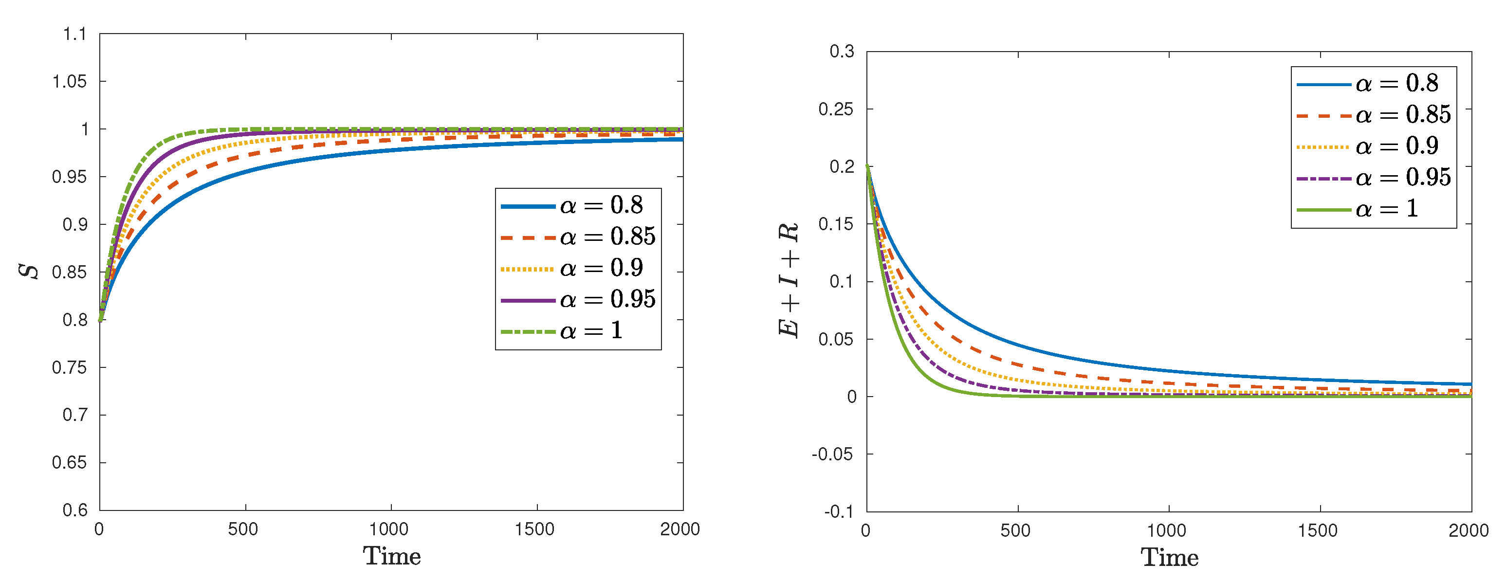
Figure 1. Stability of the disease free equilibrium Σ 0 = ( 1 , 0 , 0 , 0 ) , for the SEIR fractional model (3), considering different values of α { 0.8 , 0.85 , 0.9 , 0.95 , 1.0 } . On the left: S. On the right: E + I + R .
Axioms 10 00238 g001
Figure 2. Global stability of the disease free equilibrium Σ 0 = ( 1 , 0 , 0 , 0 ) , for the fractional model (3), considering α = 0.9 and different initial conditions x i , i = 0 , , 7 , from (5). On the left S and on the right E + I + R .
Axioms 10 00238 g002
Figure 3. Stability of the disease free equilibrium Σ 0 = ( Λ μ = 8 , 0 , 0 ) , for the SIRS fractional model (6). In the left: I + R , considering different values of α { 0.8 , 0.85 , 0.9 , 0.95 , 1.0 } and initial condition y 1 from (8). On the right: S and I + R , considering the initial conditions y i , i = 0 , , 4 from (8) and fixed α = 0.9 .
Axioms 10 00238 g003
Figure 4. Stability of the disease free equilibrium Σ 0 = ( 1 , 0 , 0 , 0 ) , for the SICA fractional model (9), considering different values of α { 0.8 , 0.85 , 0.9 , 0.95 , 1.0 } . On the left: S. On the right: I + C + A.
Axioms 10 00238 g004
Figure 5. Global stability of the disease free equilibrium Σ0 = (1, 0, 0, 0), for the fractional model (9), considering α = 0.9 and different initial conditions xi, i = 0, …, 7, from (12), on the x-axis S and on the y-axis I + C + A.
Axioms 10 00238 g005
Table 1. Parameter values of model (9) corresponding to R 0 = 0.1863 < 1 .
SymbolDescriptionValue
μRecruitment rate/natural death rate1/69.54
βHIV transmission rate0.05
ηAModification parameter1.3
ϕHIV treatment rate for I individuals1
ρDefault treatment rate for I individuals0.1
γAIDS treatment rate0.33
ωDefault treatment rate for C individuals0.09
dAIDS induced death rate1
Publisher’s Note: MDPI stays neutral with regard to jurisdictional claims in published maps and institutional affiliations.