Abstract
COVID-19 is a highly contagious disease which has spread across the world. A deterministic model that considers an important component of individuals with vertically transmitted underlying diseases (high-risk susceptible individuals), rather than the general public, is formulated in this paper. We also consider key parameters that are concerned with the disease. An epidemiological threshold, , is computed using next-generation matrix approach. This is used to establish the existence and global stability of equilibria. We identify the most sensitive parameters which effectively contribute to change the disease dynamics with the help of sensitivity analysis. Our results reveal that increasing contact tracing of the exposed individuals who are tested for COVID-19 and hospitalizing them, largely has a negative impact on . Results further reveal that transmission rate between low-risk/high-risk susceptible individuals and symptomatic infectious individuals and incubation rate of the exposed individuals have positive impact on . Numerical simulations show that there are fewer high-risk susceptible individuals than the general public when . This may be due to the fact that high-risk susceptible individuals may prove a bit more difficult to control than the low-risk susceptible individuals as a result of inherited underlying diseases present in them. We thus conclude that high level of tracing and hospitalizing the exposed individuals, as well as adherence to standard precautions and wearing appropriate Personal Protective Equipment (PPE) while handling emergency cases, are needed to flatten the epidemic curve.
Keywords:
high-risk susceptible individuals; contact tracing; Lyapunov functions; global stability; sensitivity analysis MSC:
34D23; 93C15; 93D20
1. Introduction
Until now, the COVID-19 pandemic remains a global concern due to the continuous increase in the number of infectious individuals. The number of confirmed cases has been growing very fast on a daily basis and it has been declared a worldwide pandemic disease. The disease started in Wuhan, Hubei Province, China, in 2020 and since then, it has spread across the world [1]. Presently, the pandemic has disrupted economies all over the world. Since December 2019, the world has reported 148,329,348 confirmed cases and 3,128,962 death cases [2]. High fever, severe chest pain, body aches, headache, difficulty in breathing, fatigue, pains, sore throat, skin rashes, running nose, taste loss, and diarrhea are the symptoms of COVID-19, but the main and most common symptoms are dry cough and fatigue [1].
With ongoing community transmission from asymptomatic infectious individuals, disease burden is expected to rise. Consequently, there will be an ongoing need for people with underlying diseases who are front-line health care workers in patient-facing roles. This is due to the fact that their work requires close personal exposure to patients with SARS-CoV-2. They are at high risk of infection contributing to further spread [3]. SARS-Cov-2 infects all susceptible individuals. However, evidence to date suggests that a group of people is at a higher risk of contacting the virus quickly than the general public, due to compromised immune system. These are people with underlying medical conditions. An underlying disease affects the immunity, nutritional status and general well-being of patients-factors that play a critical role in protecting individuals against COVID-19. The World Health Organization emphasizes that this group of individuals (high-risk susceptible individuals) must protect themselves from COVID-19 in order to protect others. Furthermore, the highly susceptible individuals experience severe symptoms that may lead to death when they contact COVID-19. In response to the pandemic, government authorities at various levels have put in place various control measures such as imposing strict mandatory lockdown, use of a face mask in public, regular hand washing, and social distancing. Therefore, in order to reduce COVID-19 spread, contact tracing of suspected infected individuals has been stepped up in several countries and detected cases are quickly placed in isolation for prompt treatment [4].
The use of mathematical models to describe the transmission and spread of COVID-19, so as to gain insights into the disease behaviour and develop strategies for its curtailment, has been extensively studied by researchers. (see in [5,6,7,8,9,10,11,12,13,14,15,16,17,18] and the references cited therein.) Our model has a unique difference from the models developed in [10,18] as follows: the authors of [18] developed a mathematical model of COVID-19 to investigate the impact of non-pharmaceutical interventions for possible control of the disease. In their model, they only considered symptomatically infected and asymptomatically infected individuals without considering some individuals in the susceptible population who are more vulnerable to the disease than the rest of the susceptible population. These are front-line health care workers, pregnant women, children and family of COVID-19 patients. For instance, any COVID-19 patient who visits hospital for medical treatment will be attended to by these health care workers and this puts them in higher risk of contacting the virus. Classifying these individuals as a risk and treating them as a genuine threat is a national priority. Furthermore, in [10], they modeled the effects of non-pharmaceutical interventions on COVID-19 spread in Kenya. Their model excludes the class of high risk susceptible individuals which is taken into account in our model. The work in [19] investigated a class of SEIRS epidemic models with a general nonlinear incidence function. Systems of differential equations are also used as HIV infection model with transitions between uninfected cells and infected cells. The classical HIV infection divided the cells population into following three main compartments depending on cell status, target cells, infected cells producing viruses, matured virus particles, and its concentrations are denoted by , and , respectively. The authors of [20] developed a nonlinear mathematical model of MERS-COV to study the dynamical behaviour of the disease with two discrete-time delays. We highlight the main objectives of the study to achieve our aim in what follows.
- (1)
- It is noteworthy to mention that the high-risk susceptible individuals that we refer to, in this paper, are individuals with vertically transmitted or inherited underlying diseases, i.e., HIV, asthma and so on. These individuals are at higher-risk of contacting COVID-19 than the rest of individuals in the population and thus the need for the inclusion of high-risk susceptible individuals in order to understand the disease dynamics.
- (2)
- Global stability analyses of the disease-free and endemic equilibrium points are derived
- (3)
- Robust sensitivity analysis of the model is performed to determine the contributory effects of the factors/parameters on the spread of COVID-19.
The rest of the paper is organized as follows. Section 2 has the model formulation and computation of basic reproduction number. In Section 3, global stability of disease-free and endemic equilibrium points are established. Sensitivity analysis of the model parameters is performed in Section 4. Some simulations are done in order to confirm our theoretical results, regarding the global stability of equilibriums, in Section 5. Section 6 wraps the modeling work with conclusion.
2. Materials and Methods
The total population size, N, is divided into eight mutually exclusive compartments; S, J, E, A, B, H, C, and R, which is interpreted as (i) low-risk susceptible individuals, (ii) high-risk susceptible individuals, (iii) exposed individuals, (iv) asymptomatic infectious individuals, (v) symptomatic infectious individuals, (vi) hospitalized individuals, (vii) death class, and (viii) recovered individuals. People with vertically transmitted or inherited disease are assumed as the high-risk susceptible individuals. Individuals in S and J can be exposed to Severe Acute Respiratory Syndrome Coronavirus 2 (SARS-CoV-2) through contact with either A or B, and we assume that the disease is faster transmitted in symptomatic infectious population than the asymptomatic infectious population, and include a variability factor . It is assumed that the transmission rate in classes S and J are the same. We also assume that individuals in H are in isolation and therefore cannot transmit the disease. We assume that new recruits enter human population by birth, immigration, or emigration at the rate . Furthermore, there is vertical transmission recruitment into class J at a rate . With contact tracing, a fraction, p, of the exposed individuals is tested for COVID-19 at a rate q and become hospitalized. A fraction of the remaining fraction of the exposed individuals who show no clinical symptoms of COVID-19 at the end of incubation period become asymptomatic at a progression rate , while the remaining fraction of the exposed individuals who show clinical symptoms at the end of incubation period becomes symptomatic at a progression rate . Fraction of low-risk and high-risk susceptible individuals who adhere to COVID-19 prevention guidelines (wearing of face masks, hand washing, and maintaining social distancing) is denoted as , while represents the expected decrease in the risk of infection due to strict and correct compliance to COVID-19 prevention guidelines by low-risk and high-risk susceptible individuals. Further, a fraction of low-risk and high-risk susceptible individuals who are on lockdown within a population is denoted as , while is the expected decrease in the risk of infection due to lock-down. The asymptomatic and symptomatic infectious individuals are hospitalized at the rates and k and recover at the rates and d. The hospitalized individuals recover at the rate but die due to COVID-19 at the rate u. The symptomatic infectious individuals also die due to COVID-19 at the rate . Dead individuals are buried at the rate a. and are the transmission rate of J and A and J and B while and are the transmission rate of S and A and S and B. We ignore the transmission route from death compartment as the likelihood of transmission when handling human remains is low [21].
Applying the assumptions, description of terms above, Table 1, Table 2 and Figure 1, the differential equations which describe the dynamics of COVID-19 are formulated below.
with initial conditions
where

Table 1.
Description of state variables of model (1)–(8).

Table 2.
Summary of the parameters.
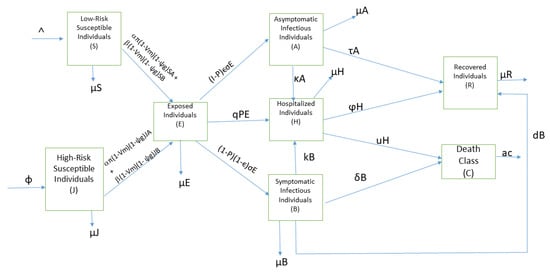
Figure 1.
Scheme of COVID-19 model.
2.1. Positivity of Solutions
Theorem 1.
Let and let the initial data for (1)–(8) be and . Then, the solutions of the model will remain non-negative for all time .
Proof.
From (1), it can be seen that
Further simplification gives
Furthermore, from (2), it can be seen that
Further simplification gives
for
We can use similar arguments to show that □
Therefore, the model (1)–(8) is well posed and epidemiologically feasible in the region
Equations (1)–(5) are independent of H, C, and R, and therefore we decouple the compartments H, C, and R from the above equations which gives
Remark 1.
Models (1)–(8) are potentially analytically solvable by using the Lie algebra method through matrix exponentials. See in [25] and the references therein. Based on the Kolmogorov equation and the Wei–Norman method, the analytical solution for the proposed model can be obtained in terms of matrix exponentials.
2.2. Basic Reproduction Number
First, we obtain the disease-free equilibrium point as . Calculation of gives . This gives . We use the next-generation operator approach in [26] to obtain the basic reproduction number . The approach is explored on the model (9)–(13) as follows:
Considering only the disease compartments, the rate of appearance of new infections and the transition rate are given, respectively, by
where
is the maximum eigenvalue given as
This is the same as
Further simplification of gives
for
3. Global Stability Analysis
In reality, there are always small perturbations. It is of interest to know whether such deviations from steady state will lead to drastic changes or will be damped out in the advancement of time. Therefore, in what follows, we establish a global asymptotic stability of the disease-free equilibrium, that is, solution trajectories of sub-population, irrespective of where they start, converge to the disease-free equilibrium solution for . This is stated and proved below.
3.1. Global Stability of Disease-Free Equilibrium Solution
Theorem 2.
The disease-free equilibrium solution is globally asymptotically stable if and unstable if
Proof.
Consider the following linear Lyapunov function
Its time derivative along solution path of COVID-19 model (9)–(13) is
where
Because and , we have
whenever
Therefore, for and if and only if or , and . Consequently, the largest invariant set in is the singleton and by LaSalle’s Invariance Principle [27], is globally asymptotically stable. The epidemiological implication of the above result is that COVID-19 can be eradicated from the population when irrespective of the initial sizes of the sub-population of the model. □
3.2. Global Stability of Endemic Equilibrium Point
Theorem 3.
The model (9)–(13) has a unique endemic equilibrium solution whenever , and no endemic equilibrium solution otherwise.
Proof.
The following equations are satisfied by the endemic equilibrium solution :
Making , , , and the subject of formula in (14)–(18) gives
Adding (14)–(16), we get
Substituting (19)–(22) in (23) yields
From (24), we can obtain to be
Substituting in (19)–(22) gives
Calculation of yields
The above results exist if only .
Further, we establish the global asymptotic stability of the endemic equilibrium solution by proving that solution trajectories converge to the endemic equilibrium point for . We shall carry this out by constructing a suitable Lyapunov candidate function of Goh–Volterra type (see [28,29] and the references cited therein). The result below establishes the global stability of the endemic equilibrium solution . □
Theorem 4.
If , then the endemic equilibrium of the model (9)–(13) is globally asymptotically stable in the interior of the region D.
Proof.
Given the following equations which are satisfied by the endemic equilibrium point :
Consider the following Lotka–Volterra Lyapunov function
where
The Lyapunov time derivative along the solutions of the model gives
Further simplification gives
Substituting and by their values and employing (29)–(33) gives
Using (29)–(35), we have
By arithmetic-geometric means inequality, i.e., , where and , it follows that with if and only if , , , , .
Therefore, the largest compact invariant subset of the set where is
Therefore, by stability theorem of Lyapunov and LaSalle’s Invariance Principle, it follows that every solution in D approaches for as .
The implication of the above result is that COVID-19 will establish itself in the population for . □
4. Sensitivity Analysis
We perform a sensitivity analysis of COVID-19 model in order to determine the parameters that are most influential in the transmission dynamics and spread of the disease. Sensitivity analysis is helpful for experimental design, data assimilation, and reduction of complex nonlinear models. A very high sensitivity indicates that more care should be taken in the estimation of the associated parameters. Following the approach in [30], we define sensitivity index of a variable to a parameter as the ratio of relative change in the variable to the relative change in the parameter.
When the variable is a differentiable function of the parameter, the sensitivity index may be alternatively defined using partial derivatives.
Definition 1.
The normalized forward sensitivity index of a variable, u(p), that depends differentiably on a parameter, p, is defined as
for
Consequently, we derive analytical expression for the sensitivity index of as
where denotes each parameter involved in
is defined as
We have Table 3 which summarizes the sensitivity indices on with respect to parameters, i.e.,

Table 3.
Numerical values of sensitivity indices of with respect to parameter involved.
In order to know the most influential parameters concerned with the basic reproduction of the disease, sensitivity analysis is performed. We categorize the most sensitive parameters in descending order to the least sensitive ones in Table 3, after ranking the sensitivity functions. The most sensitive parameters that have positive indices on are the recruitment rate , followed by the transmission rate between low-risk/high-risk susceptible individuals and symptomatic infectious individuals , followed by the incubation rate , followed by the transmission rate between low-risk/high-risk susceptible individuals and asymptomatic infectious individuals , followed by vertically transmitted recruitment rate . From the sensitivity analysis results, we can confidently say that the intervention strategies must focus on the reduction in the above parameters in order to have a disease-free population. On the other hand, the most sensitive parameters in a negative sense is the natural death rate , followed by the fraction of the exposed individuals who are tested for COVID-19 p and become hospitalized, followed by the lockdown efficacy for low and high risk susceptible individuals m, followed by the fraction of low-risk and high-risk susceptible individuals who are on lockdown , followed by the fraction of the exposed individuals who become asymptomatic , followed by rate of testing q, followed by hospitalization rate of symptomatic k, followed by effectiveness of adherence for low-risk and high-risk susceptible individuals g, followed by the recovery rate of symptomatic individuals d, followed by the fraction of low-risk and high-risk susceptible individuals who adhere to prevention guidelines , followed by hospitalization rate of asymptomatic infectious individuals , followed by COVID-19-caused death rate , followed by recovery rate of asymptomatic infectious individuals . It is clear to see that a fraction p, of the exposed individuals who are tested for COVID-19 at a rate q, and become hospitalized, has significant contribution to the disease dynamics. Therefore, high level of contact tracing through testing and hospitalization of the exposed individuals who are tested for COVID-19, are needed at the beginning of the epidemic. The sensitivity indices of the model (9)–(12) are graphically shown in Figure 2.
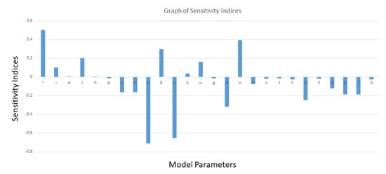
Figure 2.
Sensitivity analysis between and its associated parameters.
5. Numerical Simulations
Numerical simulations for COVID-19 model are presented in this section with the parameters mostly taken from the literature. See Table 1 and Table 2 for the description of variables and parameters with their values. Figure 3 represents the solution trajectories of the model for initial conditions , when , and so that . From Figure 3, it can be seen that the population of exposed individuals E, asymptomatic infectious individuals A, symptomatic infectious individuals B, hospitalized individuals H, and death class C converge to disease-free equilibrium solution and never turn to epidemic for and this gives an increase in the population of low-risk susceptible individuals S and high- risk susceptible individuals. This implies that COVID-19 is cleared from the population for as shown in Theorem 2. It can be viewed that the graph of high risk susceptible individuals J do not rise as much as the graph of low risk susceptible individuals S. This may be due to the fact that the high risk susceptible individuals may prove a bit more difficult to control than the low risk susceptible individuals due to their constant and inevitable exposure to the virus. Figure 4 presents the solution trajectories when = 300,000, and for initial conditions , so that . From Figure 4, it can be seen that irrespective of the initial size of the infectious population, the infectious individuals remain in the population for . Therefore, the limit of the solution trajectories is the endemic equilibrium solution. This implies that solution trajectories converge to the endemic equilibrium point. Thus, as established in Theorem 4, the disease establishes itself in the population.
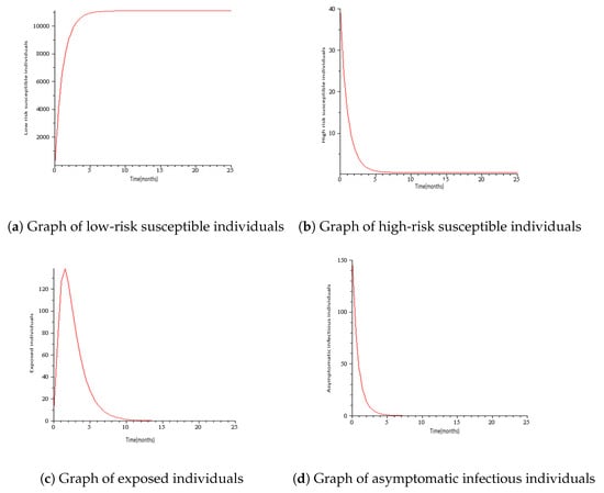
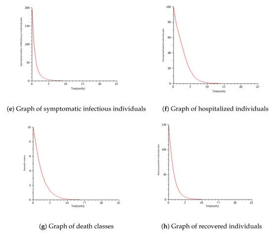
Figure 3.
Simulation results showing the global stability of the disease-free equilibrium.
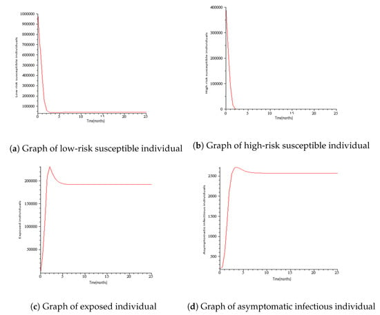
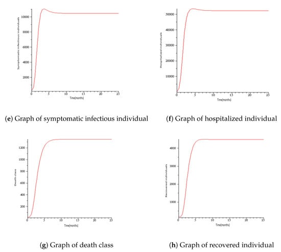
Figure 4.
Simulation results showing the global stability of the endemic equilibrium.
6. Conclusions
We have developed an epidemic model for the transmission dynamics of COVID-19. Previous research in the literature has concentrated on mathematical modeling of COVID-19, taking into account, the general public (susceptible population) without considering individuals with vertically transmitted underlying diseases (high-risk susceptible individuals), on the disease dynamics. Therefore, we formulate a mathematical model that incorporates a very important factor of individuals with higher risk of contacting the disease rather than the general public. These include HIV patients, HCV patients, asthma patient etc. The epidemiological threshold quantity, , is derived and we establish that our model has a globally asymptotic stable disease-free equilibrium solution whenever . For the case where , we have proved that there exists a unique endemic equilibrium solution, which is proved analytically to be globally asymptotically stable. We illustrate that COVID-19 disappears from the population when but persists in the population for . See Figure 3 and Figure 4. Numerical simulations reveal two equilibria: disease-free equilibrium solution and endemic equilibrium solution, which are shown to be globally asymptotically stable for and . We perform the sensitivity analysis of the basic reproduction number to each of the parameters to explore the significance of each parameter to . Sensitivity analysis results reveal that increase in the fraction of exposed individuals who are tested for COVID-19, through contact tracing, largely has negative impact on . Therefore, in order to reduce the continuous increase in the spread of the disease in the population, increase in the effective contact tracing of the exposed individuals through testing must be activated. Then, the problem of limited hospital spaces should be addressed in order to absorb higher number of COVID-19 cases. It is also pertinent that the front-line health care workers who have underlying diseases, some of which are funeral directors and mortuary personnel, who handle the bodies of those confirmed to have died from COVID-19, should avoid unnecessary manipulation of the body that may expel air from the lungs. This study can help epidemiologists and public health officials to focus more on the parameters in formulating a disease control policy. This work can be extended by placing control on the most sensitive parameter in the model so as to know the duration of time to apply control for the disease to die out. This can be achieved through optimal control analysis. It can also be extended by considering the role of high risk susceptible population on the spread of COVID-19 in a meta-population model.
Author Contributions
T.S.F. carried out the modeling and analyses. L.N.N. and T.T.M. provided data and its processing. All authors have read and agreed to the published version of the manuscript.
Funding
There is no external funding for this research. The APC was funded by the authors.
Institutional Review Board Statement
Not applicable.
Informed Consent Statement
Not applicable.
Data Availability Statement
The article contains the data used to support the findings of this study.
Acknowledgments
The authors thank the Computer Science Department of Lead City University, Nigeria, for provision of conducive space to carry out this research as well as University of Yaounde I, Cameroon.
Conflicts of Interest
The authors declare no conflict of interest.
References
- WHO. Q and A on Coronaviruses (COVID-19). Available online: https://www.who.int/emergencies/diseases/novel-coronavirus-2019/question-and-answers-hub/q-a-detail/q-a-coronaviruses (accessed on 16 July 2020).
- World Health Organization. Coronavirus (COVID-19 Dashboard). Available online: https://covid19.who.int/?adgroupsurvey=adgroupsurveygclid=EAIaIQobChMIp9yer5Ta8gIVJ8BMAh3xnw8WEAAYASABEgItCvD_BwE (accessed on 28 April 2021).
- CDC. COVID-19 response team, characteristic of health care personnel with COVID-19: United States. MMWR Morb. Mortal. Wkly. Rep. 2020, 69, 477–481. [Google Scholar]
- Dunford, D.; Dale, B.; Stylianou, N.; Lowther, E.; Ahmed, M.; Arenas, I.D.l. Coronavirus: The World in Lock-Down in Maps and Charts. BBC News, 7 April 2020. [Google Scholar]
- Adewole, M.O.; Onifade, A.A.; Abdullahi, F.A.; Kasali, F.; Ismail, A.I.M. Modeling the dynamics of COVID-19 in Nigeria. Int. J. Appl. Comput. Math. 2021, 7. [Google Scholar] [CrossRef] [PubMed]
- Dwomoh, D.; Iddi, S.; Adu, B.; Aheto, J.M.; Sedzro, K.M.; Fobil, J.; Bosomprah, S. Mathematical modeling of covid-19 infection dynamics in Ghana: Impact evaluation of integrated government and individual level interventions. Infect. Dis. Model. 2021, 6, 381–397. [Google Scholar] [PubMed]
- DarAssi, M.A.; Safi, M.A.; Ahmad, M. Global dynamics of discrete-time MERS-CoV model. Mathematics 2021, 563. [Google Scholar] [CrossRef]
- Enahoro, A.I.; Ngonghala, C.N.; Gumel, A.B. Will an imperfect vaccine curtail the COVID-19 pandemic in the US? Infect. Dis. Model. 2020, 5, 510–524. [Google Scholar]
- Gebremeskel, A.B.; Berhe, H.W.; Atsbaha, H.A. Mathematical modeling and analysis of covid-19 epidemic and predicting its future situation in Ethiopia. Results Phys. 2021, 22, 103853. [Google Scholar] [CrossRef]
- Gathungu, D.K.; Ojiambo, V.N.; Kimathi, M.E.M.; Mwalili, S.M. Modeling the effect of non-pharmaceutical interventions on Covid-19 spread in Kenya. Interdiscip. Perspect. Infect. Dis. 2020. [Google Scholar] [CrossRef]
- Iwuoha, V.C.; Aniche, E.T. COVID-19 lockdown and physical distancing policies are elitist:towards an indigenous (Afro-centred) approach to containing the pandemic in sub-urban slums in Nigeria. Local Environ. 2020, 25, 631–640. [Google Scholar] [CrossRef]
- Mohsen, A.A.; Al-Hussein, H.F.; Zhou, X.; Hattaf, K. Global stability of covid-19 model involving the quarantine strategy and media coverage effects. AIMS Public Health 2020, 7, 587–605. [Google Scholar] [CrossRef]
- Nkamba, L.N.; Manyombe, M.L.M.; Manga, T.T.; Mbang, J. Modeling Analysis of a SEIQR Epidemic Model to Assess the Impact of Undetected Cases and Containment Measures of the COVID-19 Outbreak in Cameroon. Lond. J. Press 2020, 20. [Google Scholar] [CrossRef]
- Olaniyi, S.; Obabiyi, O.S.; Okosun, K.O.; Oladipo, A.T.; Adewale, S.O. Mathematical Modeling and Optimal Cost-Effectiveness Control of COVID-19 Transmission Dynamics. Eur. Phys. J. Plus 2020, 135, 938. [Google Scholar] [CrossRef]
- Riyapan, P.; Shuaib, S.E.; Intarasit, A. A Mathematical model of COVID-19 pandemic: A case study of Bangkok, Thailand. Comput. Math. Methods Med. 2021, 11. [Google Scholar] [CrossRef]
- Shahrear, P.; Rahman, S.M.S.; Nahid, M.D.H. Prediction and mathematical analysis of the outbreak of coronavirus (covid-19) in Bangladesh. Results Appl. Math. 2021, 10. [Google Scholar] [CrossRef]
- Sinan, M.; Ali, A.; Shah, K.; Assiri, T.A.; Nofai, T.A. Stability analysis and optimal control of covid-19 pandemic SEIQR fractional mathematical model with harmonic mean type incidence rate and treatment. Results Phys. 2021, 22, 103873. [Google Scholar] [CrossRef]
- Ullah, S.; Khan, M.A. Modeling the impact of non-pharmaceutical interventions on the dynamics of novel coronavirus with optimal control analysis with a case study. Chaos Solitons Fractals 2020, 139, 110075. [Google Scholar] [CrossRef]
- Fan, X.; Wang, L.; Teng, Z. Global dynamics for a class of discrete SEIRS (susceptible-exposed-infected-recovered-susceptible) epidemic model with general nonlinear incidence. Adv. Differ. Equ. 2016, 123. [Google Scholar] [CrossRef] [Green Version]
- Batarfi, H.; Elaiw, A.; Alshareef, A. Dynamical behaviour of MERS-COV model with discrete delays. J. Comput. Anal. Appl. 2019, 26, 37–49. [Google Scholar]
- European Centre for Disease Prevention and Control. Considerations Related to the Safe Handling of Bodies of Deceased Person with Suspected or Confirmed COVID-19; ECDC: Stockholm, Sweden, 2020. [Google Scholar]
- Iboi, E.A.; Sharomi, O.O.; Ngonghala, C.N.; Gumel, A.B. Mathematical modeling and analysis of COVID-19 pandemic in Nigeria. medRxiv 2020. [Google Scholar] [CrossRef]
- Tridip, S.; Nadim, S.K.S.; Joydev, C. Assessment of 21 days lockdown effect. arXiv 2020, arXiv:2004.03487. [Google Scholar]
- Ahmad, M.D.; Usman, M.; Khan, A.; Imran, M. Optimal control analysis of Ebola disease with control strategies of quarantine and vaccination. Infect. Dis. Poverty 2016, 5, 1–2. [Google Scholar] [CrossRef] [Green Version]
- Shang, Y. Lie algebra method for solving biological population model. J. Theor. Appl. Phys. 2013, 7. [Google Scholar] [CrossRef] [Green Version]
- Diekmann, O.; Heesterbeak, J.A.P.; Metz, J.A.J. On the definition and computation of the basic reproduction ratio, R0, in models for infectious diseases in heterogeneous populations. J. Math. Biol. 1990, 284, 365–382. [Google Scholar]
- Lasalle, J.P. The Stability of Dynamical Systems; SIAM: Philadelphia, PA, USA, 1976. [Google Scholar]
- Mathur, K.S.; Narayan, P. Dynamics of an SVEIRS epidemic model with vaccination and standard incidence rate. J. Appl. Comput. Math. 2018, 118. [Google Scholar] [CrossRef]
- Guo, H.; Li, M.Y. Global stability in a mathematical model of tuberculosis. Can. Appl. Math. Quaterly 2006, 4. [Google Scholar] [CrossRef]
- Arriola, L.M.; Hyman, J.M. Being sensitive to uncertainty. J. Comput. Eng. 2007. [Google Scholar] [CrossRef]
Publisher’s Note: MDPI stays neutral with regard to jurisdictional claims in published maps and institutional affiliations. |
© 2021 by the authors. Licensee MDPI, Basel, Switzerland. This article is an open access article distributed under the terms and conditions of the Creative Commons Attribution (CC BY) license (https://creativecommons.org/licenses/by/4.0/).