Non-Standard Discrete RothC Models for Soil Carbon Dynamics

Abstract

Soil Organic Carbon (SOC) is one of the key indicators of land degradation. SOC positively affects soil functions with regard to habitats, biological diversity and soil fertility; therefore, a reduction in the SOC stock of soil results in degradation, and it may also have potential negative effects on soil-derived ecosystem services. Dynamical models, such as the Rothamsted Carbon (RothC) model, may predict the long-term behaviour of soil carbon content and may suggest optimal land use patterns suitable for the achievement of land degradation neutrality as measured in terms of the SOC indicator. In this paper, we compared continuous and discrete versions of the RothC model, especially to achieve long-term solutions. The original discrete formulation of the RothC model was then compared with a novel non-standard integrator that represents an alternative to the exponential Rosenbrock–Euler approach in the literature.

1. Introduction

The United Nations Convention to Combat Desertification (UNCCD) is an international agreement, established in 1994, that links the environment and development with sustainable land management. The first objective indicated in the UNCCD 2018–2030 Strategic Framework is to improve the conditions of affected ecosystems, combat desertification/land degradation and promote sustainable land management [1]. For each country, the commitment is to achieve no net loss of land-based natural capital by 2030 [2]. No net loss means that the quantity and quality of land-based natural capital are maintained or increased, despite the impacts of global environmental change, whether due to human or natural causes. Land degradation is monitored through the changes of the values of a specific set of consistently measured indicators from their baseline quantities, conventionally identified as their initial values. The deviations from the baseline values of these indicators are the basis for monitoring land degradation.

Soil Organic Carbon (SOC) is one key indicator of land degradation [3]. Monitoring the SOC stocks and the loss of soil organic carbon due to land use changes is fundamental for maintaining the physical, chemical and biological quality of soil [4]. Soil organic carbon positively affects soil functions with regard to habitats, biological diversity, soil fertility, crop production potential, erosion control and water retention. A high SOC content improves the processes of soil formation, nutrient storage, water holding capacity and the absorption of organic or inorganic pollutants. Thus, a reduction of the SOC stock not only indicates soil degradation, but may also have potential negative effects on soil-derived ecosystem services.

Starting from the SOC baseline, predictive spatial modelling can simulate the carbon dynamics, estimate carbon sequestration under the actual land use and evaluate the deviation from the baseline average value of total carbon [5]. Moreover, a dynamical model may determine the optimal potential land use pattern that is suitable to achieve land degradation neutrality in terms of SOC indicator values. Well-validated models, such as Rothamsted Carbon (RothC) [6], CENTURY [7] and MOMOS [8], which take into account the interactions among the climate, pedology, cropping systems and soil and crop management, can be used to predict SOC changes under different management practices and climatic conditions. These models are essentially compartmental, meaning that they represent soil organic matter as a few discrete compartments (generally two to five) characterized by different chemical characteristics of the soil’s degradation. The decomposition rates, applied to each compartment, are governed by kinetic and stoichiometric laws and are mainly ruled by the environmental conditions (e.g., soil moisture level, aeration and soil temperature). These models are used in a variety of ways and often for long-term studies. Indeed, being able to compute and predict long-term solutions is extremely valuable for various reasons: it gives a synthetic view of the system in the given agro-climatic conditions; it makes it possible to test if a studied soil has reached equilibrium or not; and it allows envisioning what would be the consequences of specific events on a given soil [9]. In this paper, we compared continuous and discrete versions of the RothC model, especially regarding long-term solutions. Moreover, since the discrete RothC version can be interpreted as a first-order approximation of the continuous model, we introduced a non-standard discrete approximation that can be interpreted as a novel discrete model of soil carbon dynamics. The original discrete formulation of the RothC model was then compared to the novel non-standard integrator, which represents a different approach with respect to the Exponential Rosenbrock–Euler (ERE) discretization [10].

2. Rothamsted Carbon Model—Continuous Formulation

The SOC indicator is considered to be the result of the equilibrium between the inputs and outputs of the soil system. SOC contained in the organic matter is constantly built up and decomposed and is then released into the atmosphere as CO${}_2$ and recaptured through photosynthesis. Inputs in the soil organic matter decomposition model consist of two major components: living organisms’ biomass (mainly plant roots and microbial biomass) and plant and animal residues at various stages of decomposition. Outputs result from the heterotrophic respiration processes when soil organic carbon is used as an energy source by soil organisms and returned to the atmosphere as CO${}_2$ fluxes. The Rothamsted Carbon model [6,11] (RothC) is a model of carbon turnover in non-waterlogged soils [12]. Initially developed for arable soils, it was later expanded to grasslands and forests. It takes into account the effects of temperature, moisture content and soil type. The RothC model divides the soil carbon into four active compartments and one inactive, characterized by different chemical decomposition rates of degradability (see Figure 1). The Inert Organic Matter (IOM) represents the inactive pool, resistant to decomposition, which does not receive carbon (C) inputs. At each time step, incoming plant residues are split between easily Decomposable Plant Material (DPM) and Resistant Plant Material (RPM), depending on the ratio ${\displaystyle \frac{\gamma }{1-\gamma }}$, which estimates the decomposability of the particular plant material inputs, which in turn depends on the specific cultivation being considered. The fraction $2\eta$ of the input of Farmyard Manure (FYM), if any, is equally split between the DPM and RPM compartments; the remaining part $1-2\eta$ enters in the system directly as Humified organic matter (HUM). Both DPM and RPM decompose to form CO${}_2$, microbial Biomass (BIO) and more HUM. The fraction $\alpha +\beta$ of metabolised C incorporated into the sum of compartments BIO+HUM is determined by the clay content of the soil, while the remaining part $1-\alpha -\beta$ is released as CO${}_2$ and lost by the system. The BIO+HUM carbon content is then split into ${\displaystyle \frac{\alpha }{\alpha +\beta }}$ percent BIO and ${\displaystyle \frac{\beta }{\alpha +\beta }}$ percent HUM. Finally, both BIO and HUM decompose to form more CO${}_2$, BIO and HUM.

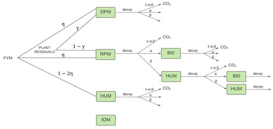
Figure 1. Flow diagram of the Rothamsted Carbon (RothC) model. FYM, Farmyard Manure; DPM, Decomposable Plant Material; RPM, Resistant Plant Material; BIO, microbial Biomass; HUM, Humified organic matter; IOM, Inert Organic Matter.

The four active compartments undergo decomposition as a function of different rate constants, which correspond to the entries of the vector $\mathbf{k}=[k_{dpm},k_{rpm},k_{bio},k_{hum}]$ and of the rate modifier $\rho \left(t\right)$, which depends on the clay content of the soil, on climatic variables (rainfall, temperature, open pan evaporation) and land cover.

In real soil systems, processes involved in the RothC model are continuous in time, and thus, in [10], the author proposed the following continuous formulation:

$$\dot{\mathbf{c}}=\rho \left(t\right)A\mathbf{c}+\mathbf{b}\left(t\right),\mathbf{c}\left(t_0\right)={\mathbf{c}}_0\ge 0$$

(1)

where $\mathbf{c}\left(t\right)={[c_{dpm}\left(t\right),c_{rpm}\left(t\right),c_{bio}\left(t\right),c_{hum}\left(t\right)]}^T$ and ${\mathbf{c}}_0\ge 0$ denotes the vector of the initial concentrations. The matrix A is given by:

$$A=\left(\begin{array}{cccc}-k_{dpm}& 0& 0& 0\\ \\ {\displaystyle 0}& -k_{rpm}& 0& 0\\ \\ {\displaystyle \alpha k_{dpm}}& \alpha k_{rpm}& (\alpha -1)k_{bio}& \alpha k_{hum}\\ \\ {\displaystyle \beta k_{dpm}}& \beta k_{rpm}& \beta k_{bio}& (\beta -1)k_{hum}\end{array}\right).$$

The vector $\mathbf{b}\left(t\right)$ represents the carbon amount entering the system at time t. It considers both the input of plant residues $g\left(t\right){\mathbf{a}}^{\left(g\right)}$ and the input of FYM $f\left(t\right){\mathbf{a}}^{\left(f\right)}$, so that:

$$\mathbf{b}\left(t\right):=g\left(t\right){\mathbf{a}}^{\left(g\right)}+f\left(t\right){\mathbf{a}}^{\left(f\right)}.$$

The entries of vectors ${\mathbf{a}}^{\left(g\right)}:={[\gamma ,1-\gamma ,0,0]}^T$ and ${\mathbf{a}}^{\left(f\right)}:={[\eta ,\eta ,0,1-2\eta ]}^T$ are the fraction inputs $0\le \gamma \le 1$, $0\le \eta \le 1/2$, which sum up to one; the carbon of plant residues enters the soil only through the DPM and RPM compartments, while the carbon amount of FYM enters through the DPM, RPM and HUM compartments.

It can be shown that, under the hypothesis $0<\alpha +\beta \le 1$ and $\rho \left(t\right)>0$, the solution of the homogeneous part of the RothC system (1) with non-negative initial data verifies the more general assumptions stated in [13,14] for biochemical systems, which ensure the well-posedness and positivity of the solution. Comparison theorems guarantee the positivity of the solution of the complete RothC system when $g\left(t\right),f\left(t\right)$ are assumed positive.

Definition 1.

We define as the SOC indicator of the continuous RothC model (1) the function $SOC\left(t\right)=c_{iom}+c_{dpm}\left(t\right)+c_{rpm}\left(t\right)+c_{bio}\left(t\right)+c_{hum}\left(t\right)$ for $t\ge t_0$, where $c_{iom}$ denotes the constant carbon content in the compartment IOM.

Theorem 1.

Let $\alpha ,\beta >0$ and $\delta :=1-\alpha -\beta >0$; suppose $0<g\left(t\right)+f\left(t\right)\le B$ and $\rho \left(t\right)$ are uniformly bounded from below by a constant $\mu >0$. The set:

$$\Omega =\left\{{\displaystyle (c_{dpm},c_{rpm},c_{bio},c_{hum})\in R_{+}^4:0\le (c_{dpm}+c_{rpm}+c_{bio}+c_{hum})\le \frac{B}{\mu \delta k_{min}}}\right\}$$

with $k_{min}={min}_i\mathbf{k}\left(i\right)$ is positively invariant and globally attractive for Model (1).

Proof. 

By denoting $\omega \left(t\right)=SOC\left(t\right)-c_{iom}$, from System (1), and recalling that ${\mathbf{e}}^T{\mathbf{a}}^{\left(g\right)}={\mathbf{e}}^T{\mathbf{a}}^{\left(f\right)}=1$, we can show that:

$$\dot{\omega }={\mathbf{e}}^T\dot{\mathbf{c}}=\rho \left(t\right){\mathbf{e}}^{T}A\mathbf{c}+g{\mathbf{e}}^T{\mathbf{a}}^{\left(g\right)}+f{\mathbf{e}}^T{\mathbf{a}}^{\left(f\right)}=g\left(t\right)+f\left(t\right)-\rho \left(t\right)\delta {\mathbf{k}}^T\mathbf{c}$$

(2)

where $\mathbf{e}={[1,1,1,1]}^T$. Consequently,

$$\dot{\omega }\le g\left(t\right)+f\left(t\right)-\rho \left(t\right)\delta k_{min}\omega \le B-\mu \delta k_{min}\omega$$

so that:

$${\displaystyle \omega \left(t\right)\le \frac{B}{\mu \delta k_{min}}-\left[{\displaystyle \frac{B}{\mu \delta k_{min}}-\omega \left(t_0\right)}\right]e^{-\mu \delta k_{min}(t-t_0)}.}$$

Therefore, if ${\displaystyle \omega \left(t_0\right)\le \frac{B}{\mu \delta k_{min}}}$, then ${\displaystyle \omega \left(t\right)\le \frac{B}{\mu \delta k_{min}}}$, with $\Omega$, resulting in a positively invariant set for model (1). Moreover, if ${\displaystyle \omega \left(t_0\right)\ge \frac{B}{\mu \delta k_{min}}}$, then ${\displaystyle {lim}_{t\to \infty }\omega \left(t\right)\le \frac{B}{\mu \delta k_{min}}}$ and $\Omega$ is globally attractive for Model (1).  □

Under the hypothesis of Theorem 1, the set:

$${\Omega }_{SOC}=\left\{{\displaystyle SOC\in R_{+},c_{iom}\le SOC\le c_{iom}+\frac{B}{\mu \delta k_{min}}}\right\}$$

is globally attractive for the SOC model:

$$\dot{SOC}={\mathbf{e}}^T\dot{\mathbf{c}}=\rho \left(t\right){\mathbf{e}}^{T}A\mathbf{c}+g\left(t\right)+f\left(t\right).$$

(3)

Finally, to complete the understanding of the mathematical features of the RothC model, we provide the following theorem:

Theorem 2.

Suppose $g\left(t\right)$ and $f\left(t\right)$ are integrable on every finite subinterval of $[t_0,+\infty )$. If $\alpha +\beta =1$, then ${\displaystyle SOC\left(t\right)=SOC\left(t_0\right)+{\int }_{t_0}^t(g\left(s\right)+f\left(s\right))ds}$.

Proof. 

Under the assumption $\alpha +\beta =1$, the unit vector $\mathbf{e}\in ker\left(A^T\right)$. We have $\dot{SOC}={\mathbf{e}}^T\dot{\mathbf{c}}=\rho {\mathbf{e}}^{T}A\mathbf{c}+g{\mathbf{e}}^T{\mathbf{a}}^{\left(g\right)}+f{\mathbf{e}}^T{\mathbf{a}}^{\left(f\right)}=g+f.$  □

Long-Term Solutions

When the RothC model is used in real application, the first step is to run the model to equilibrium to calculate the required carbon inputs needed to match the initial SOC content measured. Hence, being able to compute and predict the long-term solution are extremely valuable in order to avoid long-run simulations, which can lead to numerical artefacts if numerical tools are not properly used [15].

We firstly consider the (unrealistic) case when no CO${}_2$ release (i.e., $\alpha +\beta =1$) is considered.

Theorem 2 indicates that:

• if there is no external carbon input ($g=f=0$), then the SOC indicator is a linear invariant for the SOC model (3);
• if the carbon input $g+f$ is replaced by its average value $\widehat{g}+\widehat{f}$, then $SOC\left(t\right)$ grows linearly in time;
• if $g\left(t\right)$ and $f\left(t\right)$ are integrable on every finite subinterval of $[t_0,+\infty )$ and the improper integral ${\int }_{t_0}^{+\infty }(g\left(s\right)+f\left(s\right))ds$ converges to its value $C_{\infty }$, the indicator $SO{C}_R\left(t\right)$ increases in time tending to the finite amount $SO{C}^{*}:=SOC\left(t_0\right)+C_{\infty }$ (steady-state solution);
• if both $g\left(t\right)$ and $f\left(t\right)$ are integrable on every finite subinterval of $[t_0,+\infty )$ and ${\int }_{t_0}^t(g\left(s\right)+f\left(s\right))ds$ is a bounded periodic function of period T, then $SOC\left(t\right)$ oscillates indefinitely with period T (periodic solution).

Theorem 3.

Suppose $\alpha ,\beta ,\delta >0$ with $\alpha +\beta <1$ and $\mathbf{k}\left(i\right)>0$, $i=1,\dots 4$. For $\rho ,g,f$, not varying with time, the RothC model admits a unique positive globally stable equilibrium, which has the following expression:

$${\mathbf{c}}_{cont}^{*}={\displaystyle \frac{1}{\rho }}{\left[{\displaystyle \frac{g\gamma +f\eta }{k_{dpm}}},{\displaystyle \frac{g(1-\gamma )+f\eta }{k_{rpm}}},{\displaystyle \frac{(g+f)\alpha }{k_{bio}\delta }},{\displaystyle \frac{f(1-\alpha )(1-2\eta )+\beta (g+2f\eta )}{k_{hum}\delta }}\right]}^{⊺}.$$

(4)

Consequently, the $SOC$ indicator has ${\displaystyle SO{C}_{cont}^{*}=c_{iom}+{\mathbf{e}}^T{\mathbf{c}}_{cont}}$ as the equilibrium, which satisfies $SO{C}_{cont}^{*}\le c_{iom}+{\displaystyle \frac{f+g}{\rho k_{min}\delta }}$.

Proof. 

From the assumptions, it follows that $0<\alpha ,\beta <1$. The eigenvalues of the matrix A are given by ${\lambda }_1=-k_{dpm}<0$, ${\lambda }_2=-k_{rpm}<0$, and ${\lambda }_{3,4}$ are the roots of the second0order polynomial:

$${\lambda }^2+\lambda \left(k_{bio}(1-\alpha )+k_{hum}(1-\beta )\right)+\delta k_{bio}{k}_{hum}$$

with discriminant $\Delta \left(\lambda \right)={(\alpha -1)}^2{k}_{bio}^2+{(\beta -1)}^2{k}_{hum}^2+2k_{bio}{k}_{hum}(\alpha (\beta +1)+\beta -1)>0$. Consequently, from Descartes’ rule of sign, ${\lambda }_3,{\lambda }_4<0$. The matrix A turns out to be negative definite and admits an inverse. It is trivial to check that ${\displaystyle det\left(A\right)=\delta \prod _{i=1}^4\mathbf{k}\left(i\right)>0.}$ For constant (positive) values of $\rho ,g,f$, the equilibrium is achieved by solving the linear system $\rho A\mathbf{c}=-\mathbf{b}$, i.e.,

$${\mathbf{c}}_{cont}^{*}=-{\displaystyle \frac{1}{\rho }}{A}^{-1}\mathbf{b},$$

(5)

with:

$$-A^{-1}={\displaystyle \frac{1}{det\left(A\right)}}\left(\begin{array}{cccc}\delta k_{2,3,4}& 0& 0& 0\\ \\ 0& \delta k_{1,3,4}& 0& 0\\ \\ \alpha k_{1,2,4}& \alpha k_{1,2,4}& (1-\beta )k_{1,2,4}& \alpha k_{1,2,4}\\ \\ \beta k_{1,2,3}& \beta k_{1,2,3}& \beta k_{1,2,3}& \left(1-\alpha \right)k_{1,2,3}\end{array}\right)$$

where we adopted the convention that $k_{i,j,m}:=\mathbf{k}\left(i\right)\mathbf{k}\left(j\right)\mathbf{k}\left(m\right)$ with $i,j,m\in \{1,2,3,4\}$.

Finally, the stability of the equilibrium is guaranteed as A is negative definite.

As concerns the equilibrium of the $SOC$ indicator, first notice that, from (2), it results that ${\mathbf{k}}^T{\mathbf{c}}_{cont}^{*}={\displaystyle \frac{f+g}{\rho \delta }},$ then,

$${\displaystyle SO{C}_{cont}^{*}=c_{iom}+{\mathbf{e}}^T{\mathbf{c}}_{cont}^{*}\le c_{iom}+{\displaystyle \frac{1}{k_{min}}}{\mathbf{k}}^T{\mathbf{c}}_{cont}^{*}=c_{iom}+{\displaystyle \frac{f+g}{k_{min}\rho \delta }}.}$$

 □

When climatic and agricultural variables are considered, the functions $\rho \left(t\right)$, $g\left(t\right)$ and $f\left(t\right)$ are chosen to be time varying on a periodical basis, and the system defined by $\mathbf{c}\left(t\right)$ is expected to tend toward an oscillatory state as $t\stackrel{}{\to }+\infty$. If we introduce $\xi \left(t\right):={\int }_{t_0}^t\rho \left(s\right)ds$ for all $t\ge t_0$, then the solution of (1) is given by:

$$\mathbf{c}\left(t\right)=e^{\xi \left(t\right)A}{\mathbf{c}}_0+e^{\xi \left(t\right)A}{\int }_{t_0}^t{e}^{-\xi \left(s\right)A}\mathbf{b}\left(s\right)ds.$$

(6)

The study of the eigenvalues of $\xi \left(t\right)A$ enables characterizing the solution behaviour. We can first observe that if the eigenvalues of $A\xi \left(t\right)$ are negative, $\mathbf{c}\left(t\right)$ as $t\to +\infty$ does not depend on initial conditions ${\mathbf{c}}_0$. Secondly, if there exists a periodic solution $\mathbf{c}\left(t\right)$ with period T, then $\mathbf{c}(t_0+T)={\mathbf{c}}_0$, and the following theorem holds:

Theorem 4.

Assume that $\rho \left(t\right)$, $g\left(t\right)$ and $f\left(t\right)$ are periodic with period T. If $\alpha +\beta \ne 1$ and $\mathbf{k}\left(i\right)\ne 0$ for all $i\in [dpm,rpm,bio,hum]$, then $I-e^{\xi (t_0+T)A}$ is not singular. Starting from:

$${\mathbf{c}}_0:={(I-e^{\xi (t_0+T)A})}^{-1}{e}^{\xi (t_0+T)A}{\int }_{t_0}^{t_0+T}{e}^{-\xi \left(s\right)A}\mathbf{b}\left(s\right)ds$$

the RothC model admits a (unique) periodic solution.

Proof. 

From the periodicity of $\rho \left(t\right)$, it follows that:

$$\xi (t+T)={\int }_{t_0}^{t+T}\rho \left(s\right)ds={\int }_{t_0}^{t_0+T}\rho \left(s\right)ds+{\int }_{t_0+T}^{t+T}\rho \left(s\right)ds=\xi (t_0+T)+\xi \left(t\right).$$

By imposing in (6) that $\mathbf{c}(t_0+T)={\mathbf{c}}_0$, it follows that:

$${\mathbf{c}}_0=e^{\xi (t_0+T)A}\left({\mathbf{c}}_0+{\int }_{t_0}^{t_0+T}{e}^{-\xi \left(s\right)A}\mathbf{b}\left(s\right)ds\right).$$

(7)

Under the assumed hypothesis, A is not singular, and consequently, the matrix $I-e^{\xi (t_0+T)A}$ has the inverse. Exploiting the periodicity of $\mathbf{b}\left(t\right)$ inherited by the periodicity of both $g\left(t\right)$ and $f\left(t\right)$, we have that:

$$\begin{array}{ccc}\hfill \mathbf{c}(t+T)& =& e^{\xi (t+T)A}\left({\mathbf{c}}_0+{\int }_{t_0}^{t+T}{e}^{-\xi \left(s\right)A}\mathbf{b}\left(s\right)ds\right)\hfill \\ & =& e^{\xi \left(t\right)A}{e}^{\xi (t_0+T)A}\left({\mathbf{c}}_0+{\int }_{t_0}^{t_0+T}{e}^{-\xi \left(s\right)A}\mathbf{b}\left(s\right)ds+{\int }_{t_0+T}^{t+T}{e}^{-\xi \left(s\right)A}\mathbf{b}\left(s\right)ds\right)\hfill \\ & =& e^{\xi \left(t\right)A}{\mathbf{c}}_0+e^{\xi \left(t\right)A}{e}^{\xi (t_0+T)A}{\int }_{t_0}^t{e}^{-\xi (s+T)A}\mathbf{b}\left(s\right)ds\hfill \\ & =& e^{\xi \left(t\right)A}{\mathbf{c}}_0+e^{\xi \left(t\right)A}{\int }_{t_0}^t{e}^{-\xi \left(s\right)A}\mathbf{b}\left(s\right)ds\hfill \\ & =& \mathbf{c}\left(t\right).\hfill \end{array}$$

This proves the periodicity of $\mathbf{c}\left(t\right)$.  □

The condition $\alpha +\beta <1$ is always true for the RothC model due to the definition of $\alpha$ and $\beta$ (see [6]), and thus, the stock of carbon in each compartment tends towards a periodic solution in large times whatever the input values are.

Although the continuous approach (1) gives a simple explicit solution, the function of both the input variables and the parameters of the model, in real applications, first-order discretized versions are applied. We analyse the original discrete formulation of the RothC model, the Exponential Rosenbrock–Euler (ERE) version and a novel first-order non-standard procedure, closer to the classical discrete RothC procedure than the ERE model.

3. Non-Standard RothC Discrete Models

3.1. Original Discrete RothC

By denoting with I the identity matrix and with

$$\Lambda =\left(\begin{array}{cccc}0& 0& 0& 0\\ 0& 0& 0& 0\\ \alpha & \alpha & \alpha & \alpha \\ \beta & \beta & \beta & \beta \end{array}\right),D=\left(\begin{array}{cccc}{k}_{dpm}& 0& 0& 0\\ 0& k_{rpm}& 0& 0\\ 0& 0& k_{bio}& 0\\ 0& 0& 0& k_{hum}\end{array}\right)$$

the discrete (monthly) formulation of the RothC Version 26.3 [11] in vectorial form is given by:

$${\mathbf{c}}_{n+1}=(\Lambda +(I-\Lambda )e^{-\Delta t\rho \left(t_n\right)D}){\mathbf{c}}_n+\Delta t\mathbf{b}\left(t_n\right)$$

(8)

where ${\mathbf{c}}_n\approx \mathbf{c}\left(t_n\right)$ and the discrete temporal grid $t_{n+1}=t_0+n\Delta t$ advances with stepsize $\Delta t=1$.

Discrete RothC has been applied using data from long-term experiments across several ecosystems, climate conditions and Land Use (LU) classes. It has been extensively applied in Europe for SOC modelling, and applications of RothC to a long-term experiment in semi-arid conditions in Italy can be found in [16,17].

In the case when $g\left(t\right)$, $f\left(t\right)$ and $\rho \left(t\right)$ do not depend on time t, then $\mathbf{b}=g{\mathbf{a}}^{\left(g\right)}+f{\mathbf{a}}^{\left(f\right)}$; by setting $F(\Delta t)=\Lambda +(I-\Lambda )e^{-\Delta t\rho D}$, one can demonstrate that, whenever $\mathbf{k}\left(i\right)\ne 0$, $(I-F(\Delta t\left)\right)$ has an inverse, and the system yields a steady-state solution.

Theorem 5.

The steady-state solution ${\mathbf{c}}_{cont}^{*}$ in (5) of the continuous model (1) and the steady-state solution ${\mathbf{c}}_{RothC}^{*}(\Delta t)$ of the discrete RothC model (8) satisfy the following relation:

$${\mathbf{c}}_{cont}^{*}=\phi (-\Delta t\rho D){\mathbf{c}}_{RothC}^{*}(\Delta t)$$

where $\phi \left(z\right)=z^{-1}(e^z-1)$.

Proof. 

Firstly, evaluate $I-F(\Delta t)=(\Lambda -I)(e^{-\Delta t\rho D}-I)$. From ${\mathbf{c}}_{RothC}^{*}=F(\Delta t){\mathbf{c}}_{RothC}^{*}+\Delta t\mathbf{b}$, one can write:

$$\begin{array}{ccc}{\mathbf{c}}_{RothC}^{*}(\Delta t)\hfill & =\hfill & \Delta t{(I-F(\Delta t))}^{-1}\mathbf{b}\hfill \\ \\ \hfill & =\hfill & \Delta t{(e^{-\Delta t\rho D}-I)}^{-1}{(\Lambda -I)}^{-1}\mathbf{b}\hfill \end{array}$$

(9)

From the definition of ${\mathbf{c}}_{cont}^{*}$ in (5) and by noticing that the matrix A that defines the continuous problem (1) verifies the relation $A=(\Lambda -I)D$, it follows that:

$$\begin{array}{ccc}{\mathbf{c}}_{RothC}^{*}(\Delta t)\hfill & =\hfill & \phi {(-\Delta t\rho D)}^{-1}{\mathbf{c}}_{cont}^{*}\hfill \end{array}$$

 □

As the original discrete RothC model is applied with $\Delta t=1$, we can estimate the deviation of the equilibrium of the continuous model with respect to the equilibrium ${\mathbf{c}}_{RothC}^{*}\left(1\right)$ of the original discrete RothC model. Given the matrix norm $\parallel ·\parallel$ induced by a vector norm, as $-\rho D$ is negative definite, it results that $\parallel \phi (-\rho D)\parallel \le \parallel I\parallel =1$ and $\parallel {\mathbf{c}}_{cont}^{*}\parallel \le \parallel \phi (-\rho D){\mathbf{c}}_{RothC}^{*}\left(1\right)\parallel \le \parallel {\mathbf{c}}_{RothC}^{*}\left(1\right)\parallel$. This indicates that the equilibrium ${\mathbf{c}}_{RothC}^{*}\left(1\right)$ is, in norm, an overestimation of the theoretical equilibrium ${\mathbf{c}}_{cont}^{*}$. The relative error depends on the stepsize $\Delta t$ according to:

$${\displaystyle \frac{\parallel {\mathbf{c}}_{RothC}^{*}(\Delta t)-{\mathbf{c}}_{cont}^{*}\parallel }{\parallel {\mathbf{c}}_{cont}^{*}\parallel }}\le \parallel \phi {(-\Delta t\rho D)}^{-1}-I\parallel .$$

(10)

As concerns the equilibrium of the $SOC$ indicator, it results that:

$$SO{C}_{RothC}^{*}(\Delta t)=c_{iom}+{\mathbf{e}}^T{\mathbf{c}}_{RothC}^{*}(\Delta t)=c_{iom}+{\mathbf{e}}^T\phi {(-\Delta t\rho D)}^{-1}{\mathbf{c}}_{cont}^{*},$$

and consequently,

$$SO{C}_{RothC}^{*}(\Delta t)-SO{C}_{cont}^{*}={\mathbf{e}}^T\left(\phi {(-\Delta t\rho D)}^{-1}-I\right){\mathbf{c}}_{cont}^{*}={\mathbf{w}}^T(\Delta t){\mathbf{c}}_{cont}^{*}$$

where:

$$\mathbf{w}(\Delta t)=[{\displaystyle \frac{1-\phi (-\Delta t\rho k_{dpm})}{\phi (-\Delta t\rho k_{dpm})}},{\displaystyle \frac{1-\phi (-\Delta t\rho k_{rpm})}{\phi (-\Delta t\rho k_{rpm})}},{\displaystyle \frac{1-\phi (-\Delta t\rho k_{bio})}{\phi (-\Delta t\rho k_{bio})}},{\displaystyle \frac{1-\phi (-\Delta t\rho k_{hum})}{\phi (-\Delta t\rho k_{hum})}}]$$

(11)

a vector with positive entries that verifies ${lim}_{\Delta t\to 0}\mathbf{w}(\Delta t)=\mathbf{0}$.

Since the original discrete RothC model is applied with $\Delta t=1$, the deviation of the $SO{C}_{cont}^{*}$ of the continuous model with respect to the equilibrium $SO{C}_{RothC}^{*}\left(1\right)$ of the original discrete RothC model is given by $SO{C}_{RothC}^{*}\left(1\right)=SO{C}_{cont}^{*}+{\mathbf{w}}^T\left(1\right){\mathbf{c}}_{cont}^{*},$ thus indicating that the evaluation of soil organic carbon by means of the discrete RothC model is an overestimation of the theoretical value $SO{C}_{cont}^{*}$.

Usually, $\rho$, g and f vary through time, but it can be assumed that they have a periodic behaviour. Typically, if the agricultural practices are cyclic and if the weather conditions can be considered periodic, then $\rho =\rho \left(t\right)$, $g=g\left(t\right)$ and $f=f\left(t\right)$ will also behave periodically. Assuming that the periodicity of these variables is $T=N\Delta t$, one looks for a solution of $\mathbf{c}$ such that ${\mathbf{c}}_0={\mathbf{c}}_N$. Then, we can write:

$$\begin{array}{ccc}{\mathbf{c}}_{n+1}& =& (\Lambda +(I-\Lambda )e^{-\Delta t\rho \left(t_n\right)D}){\mathbf{c}}_n+\Delta t\mathbf{b}\left(t_n\right)\hfill \end{array}$$

for $n=0,\dots N-2$ and then impose the periodic condition ${\mathbf{c}}_N={\mathbf{c}}_0$:

$${\mathbf{c}}_0=(\Lambda +(I-\Lambda )e^{-\Delta t\rho \left(t_{N-1}\right)D}){\mathbf{c}}_{N-1}+\Delta t\mathbf{b}\left(t_{N-1}\right).$$

Setting $F_n:=F_n(\Delta t):=\Lambda +(I-\Lambda )e^{-\Delta t\rho \left(t_n\right)D}$, the above relations can be reformulated as:

$$\left(\begin{array}{ccccc}0& I& 0& \dots & 0\\ ⋮& \ddots & \ddots & \ddots & ⋮\\ ⋮& & \ddots & \ddots & 0\\ 0& \dots & \dots & 0& I\\ I& 0& \dots & 0& 0\end{array}\right)\left(\begin{array}{c}{\mathbf{c}}_0\hfill \\ {\mathbf{c}}_1\hfill \\ ⋮\hfill \\ {\mathbf{c}}_{N-2}\hfill \\ {\mathbf{c}}_{N-1}\hfill \end{array}\right)=\left(\begin{array}{ccccc}{F}_0& 0& \dots & \dots & 0\\ 0& F_1& \ddots & & \dots \\ ⋮& \ddots & \ddots & \ddots & ⋮\\ ⋮& & \ddots & \ddots & 0\\ 0& \dots & \dots & 0& F_{N-1}\end{array}\right)\left(\begin{array}{c}{\mathbf{c}}_0\hfill \\ {\mathbf{c}}_1\hfill \\ ⋮\hfill \\ {\mathbf{c}}_{N-2}\hfill \\ {\mathbf{c}}_{N-1}\hfill \end{array}\right)+\Delta t\left(\begin{array}{c}{\mathbf{b}}_0\hfill \\ {\mathbf{b}}_1\hfill \\ ⋮\hfill \\ {\mathbf{b}}_{N-2}\hfill \\ {\mathbf{b}}_{N-1}\hfill \end{array}\right)$$

which yields:

$$\left(\begin{array}{c}{\mathbf{c}}_0\hfill \\ {\mathbf{c}}_1\hfill \\ ⋮\hfill \\ {\mathbf{c}}_{N-2}\hfill \\ {\mathbf{c}}_{N-1}\hfill \end{array}\right)=-\Delta t{\left(\begin{array}{ccccc}{F}_0& -I& \dots & \dots & 0\\ 0& F_1& -I& & \dots \\ ⋮& \ddots & \ddots & \ddots & ⋮\\ ⋮& & \ddots & \ddots & -I\\ -I& \dots & \dots & 0& F_{N-1}\end{array}\right)}^{-1}\left(\begin{array}{c}{\mathbf{b}}_0\hfill \\ {\mathbf{b}}_1\hfill \\ ⋮\hfill \\ {\mathbf{b}}_{N-2}\hfill \\ {\mathbf{b}}_{N-1}\hfill \end{array}\right),$$

(12)

where ${\mathbf{b}}_n:=\mathbf{b}\left(t_n\right)$, for $n=0,\dots ,N-1$. Equation (12) provides a vector of dimension $4\times N$ and a sequence of states ${\mathbf{c}}_n={[c_n^{\left(dpm\right)},c_n^{\left(rpm\right)},c_n^{\left(bio\right)},c_n^{\left(hum\right)}]}^T$, $n=0,\dots N-1$, which characterizes the oscillatory state of the carbon stock in each compartment, keeping track of the temporal variability of the forcing variables over the period.

3.2. Exponential Rosenbrock–Euler Model

If we regard the stepping procedure in (8), which defines the original discrete RothC model as a first-order approximation of the solution of the continuous model (1), then different discrete RothC models can be formulated. As an example, the discretization of Equation (1) from $t_n=t_0+n\Delta t$ to $t_{n+1}=t_n+\Delta t$ by means of the exponential Rosenbrock–Euler model (for non-autonomous systems) [10,18,19] leads to:

$$\begin{array}{ccc}{\mathbf{c}}_{n+1}\hfill & =\hfill & e^{\Delta t\rho \left(t_n\right)A}{\mathbf{c}}_n+\Delta t\phi (\Delta t\rho \left(t_n\right)A)\mathbf{b}\left(t_n\right)\hfill \\ \\ \hfill & =\hfill & {\mathbf{c}}_n+\Delta t\phi (\Delta t\rho \left(t_n\right)A)\mathbf{f}(t_n;{\mathbf{c}}_n)\hfill \end{array}$$

(13)

where $\mathbf{f}(t;\mathbf{c}):=\rho \left(t\right)A\mathbf{c}\left(t\right)+\mathbf{b}\left(t\right)$. Notice that A is negative definite, and for $z<0$, it results in $0<\phi \left(z\right)<1$. In [10], it was shown that $A=(\Lambda -I)D$ and:

$$F_n(\Delta t)=\Lambda +(I-\Lambda )e^{-\Delta tD\rho \left(t_n\right)}\approx e^{\Delta t\rho \left(t_n\right)A},\Delta t\phi (\Delta t\rho \left(t_n\right)A)=\mathcal{O}\left(diag(\Delta t)\right).$$

Of course, the approximated solutions via the Exponential Rosenbrock–Euler (ERE) method (13) differ from the values given by the original discrete RothC model (8); the major consequence is that the constant discrete steady-state solution, which for the ERE method coincides with the continuous equilibrium ${\mathbf{c}}_{cont}^{*}$, does not depend on $\Delta t$. As concerns its stability, given A negative definite, it is enough to notice that the eigenvalues of $e^{\Delta t\rho \left(t_n\right)A}$ are positive, but all less than one.

To find periodic solutions via the ERE method, we can generalize the approach followed for the discrete original RothC model as follows. Suppose that $T=N\Delta t$, and let us impose that ${\mathbf{c}}_0={\mathbf{c}}_N$:

$$\begin{array}{ccc}{\mathbf{c}}_{n+1}& =& e^{\Delta tA\rho \left(t_n\right)}{\mathbf{c}}_n+\Delta t\phi (\Delta tA\rho \left(t_n\right))\mathbf{b}\left(t_n\right)\hfill \end{array}$$

for $n=0,\dots N-2$ and:

$${\mathbf{c}}_0=e^{\Delta tA\rho \left(t_{N-1}\right)}{\mathbf{c}}_{N-1}+\Delta t\phi (\Delta tA\rho \left(t_{N-1}\right))\mathbf{b}\left(t_{N-1}\right)$$

which yields:

$$\left(\begin{array}{c}{\mathbf{c}}_0\hfill \\ {\mathbf{c}}_1\hfill \\ ⋮\hfill \\ {\mathbf{c}}_{N-2}\hfill \\ {\mathbf{c}}_{N-1}\hfill \end{array}\right)=-\Delta t{\left(\begin{array}{ccccc}{e}^{\Delta tA\rho \left(t_0\right)}& -I& \dots & \dots & 0\\ 0& e^{\Delta tA\rho \left(t_1\right)}& -I& & \dots \\ ⋮& \ddots & \ddots & \ddots & ⋮\\ ⋮& & \ddots & \ddots & -I\\ -I& \dots & \dots & 0& e^{\Delta tA\rho \left(t_{N-1}\right)}\end{array}\right)}^{-1}\left(\begin{array}{c}{\tilde{\mathbf{b}}}_0\hfill \\ {\tilde{\mathbf{b}}}_1\hfill \\ ⋮\hfill \\ {\tilde{\mathbf{b}}}_{N-2}\hfill \\ {\tilde{\mathbf{b}}}_{N-1}\hfill \end{array}\right),$$

(14)

with ${\tilde{\mathbf{b}}}_n:=\phi (\Delta t\rho \left(t_n\right)A){\mathbf{b}}_n$, for $n=0,\dots ,N-1$.

The sequence of states ${\mathbf{c}}_n$, $n=0,\dots N-1$ characterizes the oscillatory state of the carbon stock in each compartment. Of course, the solution differs from the periodic solution provided in (12).

3.3. Novel Non-Standard Discrete RothC Model

The ERE procedure described in (13) belongs to the more general class of non-standard finite difference schemes [14,20]. Different first-order non-standard approximations can be used, depending on the function of the stepsize used to advance the first-order procedure. Each of them can be considered as discrete RothC models, alternative to the ERE model.

A discrete model, closer to the original formulation of the RothC model, can be introduced as follows. Consider the discrete formulation of RothC (8). Simple evaluations lead to the equivalent expressions:

$$\begin{array}{ccc}{\mathbf{c}}_{n+1}\hfill & =\hfill & F_n(\Delta t){\mathbf{c}}_n+\Delta t\mathbf{b}\left(t_n\right)\hfill \\ \\ \hfill & =\hfill & {\mathbf{c}}_n+\Delta t\phi (\Delta t\rho \left(t_n\right)\tilde{A})\rho \left(t_n\right)A{\mathbf{c}}_n+\Delta t\mathbf{b}\left(t_n\right)\hfill \end{array}$$

(15)

where the eigenvalues of the matrix $\tilde{A}=-A{(I-\Lambda )}^{-1}=-(I-\Lambda )D{(I-\Lambda )}^{-1}$ are the entries of the vector $-\mathbf{k}$, and the columns of:

$${(I-\Lambda )}^{-1}={\displaystyle \frac{1}{\delta }}\left(\begin{array}{cccc}\delta & 0& 0& 0\\ 0& \delta & 0& 0\\ \alpha & \alpha & \beta -1& \alpha \\ \beta & \beta & \beta & \alpha -1\end{array}\right)$$

(16)

are the corresponding eigenvectors.

A novel Non-Standard (NS) discrete RothC model is given by:

$$\begin{array}{ccc}{\mathbf{c}}_{n+1}\hfill & =\hfill & {\mathbf{c}}_n+\Delta t\phi (\Delta t\rho \left(t_n\right)\tilde{A})\mathbf{f}({\mathbf{c}}_n;t_n)\hfill \\ \\ \hfill & =\hfill & F_n(\Delta t){\mathbf{c}}_n+\Delta t\phi (\Delta t\rho \left(t_n\right)\tilde{A})\mathbf{b}\left(t_n\right)\hfill \end{array}$$

(17)

Indeed, we can prove that:

Theorem 6.

The NS model (17) is a non-standard first-order approximation of the continuous model (1), i.e.,

$$\Delta t\phi (\Delta t\rho \left(t_n\right)\tilde{A})=\mathcal{O}\left(diag(\Delta t)\right),for\Delta t\to 0.$$

Proof. 

From the definition of the exponential matrix, we have that:

$$\begin{array}{ccc}\hfill \Delta t\phi (\Delta t\rho \left(t_n\right)\tilde{A})& =& {\displaystyle \frac{1}{\rho \left(t_n\right)}}{\tilde{A}}^{-1}\left(e^{\Delta t\rho \left(t_n\right)\tilde{A}}-I\right)\hfill \\ \\ & =& {\displaystyle \frac{1}{\rho \left(t_n\right)}}{\tilde{A}}^{-1}\sum _{j=1}^{\infty }{\displaystyle \frac{1}{j!}}{\left(\Delta t\rho \left(t_n\right)\tilde{A}\right)}^j\hfill \\ \\ & =& diag(\Delta t)+{\displaystyle \frac{\Delta t^2}{2}}\rho \left(t_n\right)\tilde{A}+\sum _{j=2}^{\infty }{\displaystyle \frac{\Delta t^{j+1}}{(j+1)!}}{\left(\rho \left(t_n\right)\tilde{A}\right)}^j\hfill \end{array}$$

It follows that $\Delta t\phi (\Delta t\rho \left(t_n\right)\tilde{A})=\mathcal{O}\left(diag(\Delta t)\right),\mathrm{for}\Delta t\to 0.$  □

By comparing the ERE flow (13) with the above non-standard formulation (17), we notice that the main difference is in the replacement of the matrix A with the matrix $\tilde{A}$, which has a simple representation in Jordan form. This simplifies the evaluation of the matrix function $\phi (\Delta t\rho \left(t_n\right)\tilde{A})$ because it can be evaluated on the known eigenvalues $-\mathbf{k}\left(i\right)$ and eigenvectors in (16).

Moreover, the comparison of the original discrete formulation of the RothC model (8) with the novel NS procedure (17) allows us to notice that, different from the ERE method (13), the decomposition dynamic is now treated in the same way as the original discrete RothC model. The time updating procedure related to the carbon amount entering the system at time $t+\Delta t$ is now evaluated up to a factor given by $\phi (\Delta t\rho \left(t_n\right)\tilde{A})$, different from the ERE approximation, which advances evaluating $\phi (\Delta t\rho \left(t_n\right)A)$.

As the ERE method, in the case of constant functions $\rho ,g,f$, the novel method NS has ${\mathbf{c}}_{cont}^{*}$ as the steady-state solution.

Theorem 7.

Under the hypothesis $0<\alpha +\beta <1$, the equilibrium ${\mathbf{c}}_{cont}^{*}$ of the NS method (17) is globally stable.

Proof. 

It is enough to prove that the eigenvalues of $F_n(\Delta t)=\Lambda +(I-\Lambda )e^{-\Delta t\rho \left(t_n\right)D}$ are in modulus less than one. It is easy to see that two eigenvalues are given by $e^{-\Delta t\rho \left(t_n\right)k_{dpm}}$ and $e^{-\Delta t\rho \left(t_n\right)k_{rpm}}$. The others are the eigenvalues of the sub-matrix:

$$F_{3,4}=\left(\begin{array}{cc}\alpha -e^{-\Delta t\rho \left(t_n\right)k_{bio}}\left(\alpha -1\right)& \alpha -\alpha e^{-\Delta t\rho \left(t_n\right)k_{hum}}\\ \\ \beta -\beta e^{-\Delta t\rho \left(t_n\right)k_{bio}}& \beta -e^{-\Delta t\rho \left(t_n\right)k_{hum}}\left(\beta -1\right)\end{array}\right)$$

The eigenvalues lie in the union of the two Gershgorin sets:

$$K_1=\left\{z\in \mathbf{C}:|z-\alpha +e^{-\Delta t\rho \left(t_n\right)k_{bio}}\left(\alpha -1\right)|\le |\beta -\beta e^{-\Delta t\rho \left(t_n\right)k_{bio}}|\right\},$$

$$K_2=\left\{z\in \mathbf{C}:|z-\alpha +\alpha e^{-\Delta t\rho \left(t_n\right)k_{hum}}|\le |\beta -e^{-\Delta t\rho \left(t_n\right)k_{hum}}\left(\beta -1\right)|\right\}.$$

Notice that $F_{3,4}$ has positive entries. Set

$M=max\left(F_{3,4}(1,1)+F_{3,4}(2,1),F_{3,4}(1,2)+F_{3,4}(2,2)\right)$; if $z\in K_1\cup K_2$, then $\left|z\right|\le M$. evaluate:

$$F_{3,4}(1,1)+F_{3,4}(2,1)=(\alpha +\beta )(1-e^{-\Delta t\rho \left(t_n\right)k_{bio}})+e^{-\Delta t\rho \left(t_n\right)k_{bio}}<1$$

Similarly,

$$F_{3,4}(1,2)+F_{3,4}(2,2)=(\alpha +\beta )(1-e^{-\Delta t\rho \left(t_n\right)k_{hum}})+e^{-\Delta t\rho \left(t_n\right)k_{hum}}<1$$

Hence it results that the eigenvalue of $F_{3,4}$ are less than one in modulus.  □

To search for periodic solutions via the novel non-standard model, we need to solve the linear system:

$$-\left(\begin{array}{ccccc}{F}_0& -I& \dots & \dots & 0\\ 0& F_1& -I& & \dots \\ ⋮& \ddots & \ddots & \ddots & ⋮\\ ⋮& & \ddots & \ddots & -I\\ -I& \dots & \dots & 0& F_{N-1}\end{array}\right)\left(\begin{array}{c}{\mathbf{c}}_0\hfill \\ {\mathbf{c}}_1\hfill \\ ⋮\hfill \\ {\mathbf{c}}_{N-2}\hfill \\ {\mathbf{c}}_{N-1}\hfill \end{array}\right)=\Delta t\left(\begin{array}{c}{\widehat{\mathbf{b}}}_0\hfill \\ {\widehat{\mathbf{b}}}_1\hfill \\ ⋮\hfill \\ {\widehat{\mathbf{b}}}_{N-2}\hfill \\ {\widehat{\mathbf{b}}}_{N-1}\hfill \end{array}\right),$$

where ${\widehat{\mathbf{b}}}_n:=\phi (\Delta t\rho \left(t_n\right)\tilde{A}){\mathbf{b}}_n$, for $n=0,\dots ,N-1$. As already observed, we have the same coefficient matrix of the system (12), while the knowledge of the explicit Jordan form of the matrix $\tilde{A}$ simplifies the evaluation of the coefficients ${\widehat{\mathbf{b}}}_n$.

In the next two sections, we compare the behaviour of the different discrete models on the evaluation of steady-state and long-term periodic solutions. Firstly, the comparison is made on a theoretical basis comparing the accuracy of the methods in approximating the solutions of the continuous model; secondly, we tested both the ERE and the novel non-standard model with respect to the original discrete RothC model on a classical monthly time-scale experiment where real measurements were available.

A freely accessible MATLAB routine named NSRothC [21] was implemented to replicate all the simulations presented in the next sections. The package includes two versions. The first one (contNSRothC) allowed us to run the model with different stepsizes, when the continuous periodic input functions $\rho \left(t\right)$ and $\mathbf{b}\left(t\right)$ have the particular form presented in Section 4. In the second version (monNSRothC), the stepsize was fixed to one month, and the discrete monthly values of input residuals and FYM were required, as well as the monthly values of weather variables (temperature, rainfall and moisture). As an example, data from the Hoosfield spring barley experiment [6] were used.

4. Numerical Tests

Let us compare long-term solutions obtained by using the original discrete RothC model, the exponential Rosenbrock–Euler method and the novel non-standard first-order scheme. We set parameters $\alpha =0.1$, $\beta =0.12$, $\gamma =0.59$ and $\eta =0.49$. The vector of the decomposition rates $\mathbf{k}=[0.8333,0.0250,0.0550,0.0017]$ and functions $\rho \left(t\right)$, $g\left(t\right)$ and $f\left(t\right)$ are supposedly expressed on a monthly scale. They vary with the same period $T=12$ and have Gaussian distributions according to:

$$\rho \left(t\right)=a_{\rho }+{\displaystyle \frac{G(t,{\mu }_{\rho }^{\left(1\right)},{\sigma }_{\rho }^{\left(1\right)})}{{\displaystyle {\int }_{t_0}^{t_0+T}G(s,{\mu }_{\rho }^{\left(1\right)},{\sigma }_{\rho }^{\left(1\right)})ds}}}{b}_{\rho }^{\left(1\right)}+{\displaystyle \frac{G(t,{\mu }_{\rho }^{\left(2\right)},{\sigma }_{\rho }^{\left(2\right)})}{{\displaystyle {\int }_{t_0}^{t_0+T}G(s,{\mu }_{\rho }^{\left(2\right)},{\sigma }_{\rho }^{\left(2\right)})ds}}}{b}_{\rho }^{\left(2\right)}$$

$$g\left(t\right)=a_g+{\displaystyle \frac{G(t,{\mu }_g,{\sigma }_g)}{{\displaystyle {\int }_{t_0}^{t_0+T}G(s,{\mu }_g,{\sigma }_g)ds}}}{b}_g,f\left(t\right)=a_f+{\displaystyle \frac{G(t,{\mu }_f,{\sigma }_f)}{{\displaystyle {\int }_{t_0}^{t_0+T}G(s,{\mu }_f,{\sigma }_f)ds}}}{b}_f$$

where $G(t,\mu ,\sigma ):={\displaystyle \frac{1}{\sigma \sqrt{2\pi }}}{e}^{{\displaystyle \frac{-{\left(t-t_0-\mu -⌊{\displaystyle \frac{t-t_0}{T}}⌋T\right)}^2}{2{\sigma }^2}}}$ for $t\ge t_0$.

Values $a_{\rho }=0.3561$, ${\mu }_{\rho }^{\left(1\right)}=\frac{T}{2}$, ${\mu }_{\rho }^{\left(2\right)}=\frac{5T}{6}$ were set, amplitudes $b_{\rho }^{\left(1\right)}=0.9596$ and $b_{\rho }^{\left(2\right)}=1.4996$ were chosen, while dispersion coefficients were given by ${\sigma }_{\rho }^{\left(1\right)}={\sigma }_{\rho }^{\left(2\right)}=0.6738$. The function $\rho \left(t\right)$ in a time-span of three years is shown in Figure 2 on the left.

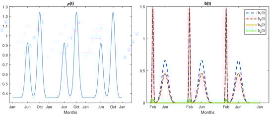
Figure 2. The function $\rho \left(t\right)$ (on the left) and the vectorial function $\mathbf{b}\left(t\right)$ (on the right) in a three-year time-span.

Values $a_g=0$, ${\mu }_g=\frac{T}{2}$, $b_g=2.7996$, ${\sigma }_g=0.9974$ define the function $g\left(t\right)$, while values $a_f=0$, ${\mu }_f=\frac{T}{6}$, $b_f=1.5$, ${\sigma }_f=0.1995$ define the function $f\left(t\right)$. The four components of the input function $\mathbf{b}\left(t\right):=g\left(t\right){\mathbf{a}}^{\left(g\right)}+f\left(t\right){\mathbf{a}}^{\left(f\right)}$ are depicted in Figure 2, on the right.

4.1. Steady-State Solution

To compare long-time periodic and steady-state solutions, we consider the average values of $\rho \left(t\right)$ and $\mathbf{b}\left(t\right)$ over one period T:

$$\begin{array}{ccc}\hfill \widehat{\rho }& =& a_{\rho }+{\displaystyle \frac{b_{\rho }^{\left(1\right)}}{T}}+{\displaystyle \frac{b_{\rho }^{\left(2\right)}}{T}}=0.5610,\hfill \\ \\ \hfill \widehat{\mathbf{b}}& =& \left(a_g+{\displaystyle \frac{b_g}{T}}\right){\mathbf{a}}^{\left(g\right)}+\left(a_f+{\displaystyle \frac{b_f}{T}}\right){\mathbf{a}}^{\left(f\right)}=0.2333{\mathbf{a}}^{\left(g\right)}+0.125{\mathbf{a}}^{\left(f\right)}={[0.1989,0.1569,0,0.025]}^T,\hfill \end{array}$$

and we evaluate the steady-state solution (4) of the continuous RothC model (1):

$${\mathbf{c}}_{cont}^{*}={[0.4254,11.1867,1.4887,61.6253]}^T.$$

(18)

We recall that both the ERE and the NS method have ${\mathbf{c}}_{cont}^{*}$ as the steady-state solution of their discrete flows, and consequently, they provide the value of $SO{C}_{cont}^{*}$ as the equilibrium for soil organic carbon; differently, the steady-state solution of the discrete RothC model (9) depends on the chosen stepsize $\Delta t$. In Table 1, we report the equilibrium solutions ${\mathbf{c}}_{RothC}^{*}(\Delta t)$ for decreasing values of the stepsize $\Delta t$. When we proceed with $\Delta t=1$, we obtain the original monthly time-stepping procedure, while $\Delta t=1/30$ represents a daily temporal updating. Notice that, as predicted by the theoretical results, $\parallel {\mathbf{c}}_{cont}^{*}{\parallel }_2=62.6516\le {\parallel {\mathbf{c}}_{RothC}^{*}\left(1\right)\parallel }_2=62.695$, i.e., the original discrete RothC model overestimates in norm the theoretical equilibrium value.

Table 1. Dependence of the steady-state solution of the discrete RothC model on the temporal stepsize $\Delta t$. The values in each compartment converge, with first-order accuracy, to the entries of ${\mathbf{c}}_{cont}^{*}={[0.4254,11.1867,1.4887,61.6253]}^T.$

$\Delta \mathit{t}$	1	$\frac{1}{5}$	$\frac{1}{10}$	$\frac{1}{15}$	$\frac{1}{20}$	$\frac{1}{25}$	$\frac{1}{30}$
${\mathbf{c}}_{RothC}^{*}$	0.5326	0.4456	0.4354	0.4321	0.4304	0.4294	0.4287
	11.2653	11.2024	11.1946	11.1919	11.1906	11.1899	11.1893
	1.5118	1.4933	1.4910	1.4902	1.4898	1.4896	1.4894
	61.6541	61.6311	61.6282	61.6272	61.6267	61.6265	61.6263

The reduction of the temporal stepsize of $1/30$ causes approximately the same reduction of the absolute errors as ${\displaystyle \frac{\parallel {\mathbf{c}}_{cont}^{*}-{\mathbf{c}}_{RothC}^{*}{\left(1\right)\parallel }_2}{\parallel {\mathbf{c}}_{cont}^{*}-{\mathbf{c}}_{RothC}^{*}{(1/30)\parallel }_2}}=31.534,$ with this confirming the first-order accuracy of the approximation of the steady-state solution. In Figure 3a, we report the relative errors ${\displaystyle \frac{\parallel {\mathbf{c}}_{cont}^{*}-{\mathbf{c}}_{RothC}^{*}{(\Delta t)\parallel }_2}{\parallel {\mathbf{c}}_{cont}^{*}{\parallel }_2}}$ in correspondence of halved stepsizes starting from $\Delta t=1$ together with their bounds evaluated in (10). In the same figure, we report the error on the equilibrium value of SOC normalized respect to ${\mathbf{c}}_{cont}^{*}$, i.e.,

$${\displaystyle \frac{SO{C}_{RothC}^{*}(\Delta t)-SO{C}_{cont}^{*}}{\parallel {\mathbf{c}}_{cont}^{*}{\parallel }_2}}={\mathbf{w}}^T(\Delta t){\displaystyle \frac{{\mathbf{c}}_{cont}^{*}}{\parallel {\mathbf{c}}_{cont}^{*}{\parallel }_2}}$$

where $\mathbf{w}(\Delta t)$ is defined in (11), with respect to the same reduction of the stepsize $\Delta t$.

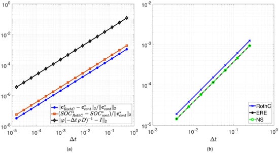
Figure 3. (a) Relative errors of ${\mathbf{c}}_{RothC}^{*}$ (blue) and ${SOC}_{RothC}^{*}$ (orange) with halved stepsizes, starting from $\Delta t=1$ The bounds on the relative error ${\parallel \phi {(-\Delta t\rho D)}^{-1}-I\parallel }_2$ in (10) are also plotted in black. The estimated order of convergence is 1.0037 for the relative error on ${\mathbf{c}}_{RothC}^{*}$ and 1.0022 for the relative error on SOC. (b) The log-log plot of the norm two errors of the periodic solutions of discrete RothC, Exponential Rosenbrock–Euler (ERE) and Non-Standard (NS) schemes, with respect to the reference solution obtained in the long run with the ode45 Matlab code, at $\Delta t=1/2^i,i=2,\dots ,8$. The estimated orders of convergence are 1.0042, 1.0017 and 1.0018 for the discrete RothC, ERE and NS schemes, respectively.

4.2. Periodic Solutions

In these experiments, we compared the periodic solutions provided by the three discrete models, obtained for the functions $\rho \left(t\right)$ and $\mathbf{b}\left(t\right)$ plotted in Figure 2. Different from the evaluation of steady-state solutions, the ERE and the novel NS procedure, as well as the discrete RothC model provide long-term periodic solutions affected by their own numerical errors, also depending on the chosen stepsize $\Delta t$. As shown in Figure 3b, the RothC discrete model provides the worst performance when compared with the other procedures in terms of errors with respect to the reference solution. In Figure 4, we plot the related SOC indicator (1) in a one-period time span obtained with the three discrete procedures applied with reduced stepsizes $\Delta t=1,1/2,1/4,1/8$. In the same figure, the reference solution obtained in the long run with the ode45 MATLAB function, with tolerance set at machine precision, is plotted. Notice that all the methods need to be applied with a $\Delta t<<1$ in order to have an acceptable level of accuracy when compared to the reference solution. Again, the original discrete RothC model was confirmed as a less accurate integrator of the continuous model (1) with respect to both the ERE and NS models.

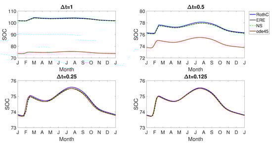
Figure 4. Periodic dynamics of the SOC indicator in a one-period span: convergence of approximated solutions to the reference solution (plotted as a continuous red line) obtained with MATLAB ode45 code, by an increasingly reduction of the stepsize $\Delta t$.

In our second experiment, we started at $t_0=1$ with ${\mathbf{c}}_0={\mathbf{c}}_{cont}^{*}$ in (18), and we proceeded until the final time $T_f=t_0+15T$ was reached. We recall that the period was set at $T=12$, and we used the monthly, weekly and daily update by setting $\Delta t=1$, $\Delta t=1/4$ and $\Delta t=1/30$, respectively. In Figure 5, we report the values of SOC obtained for the three different procedures. Two main observations have to be made: first, the initial value ${\mathbf{c}}_{cont}^{*}$ corresponding to the equilibrium solution with mean values $\widehat{\rho }$ and $\widehat{\mathbf{b}}$ was higher than the attained value of SOC reference value at $T_f$ when $\rho \left(t\right)$ and $\mathbf{b}\left(t\right)$ were not averaged. This indicates that the temporal oscillations of $\rho \left(t\right)$ and $\mathbf{b}\left(t\right)$ around their mean values cannot be neglected when evaluating, through the SOC indicator, the achievement of land degradation neutrality in the fifteen years from 2015–2030. Second, whatever discrete model is chosen, a qualitative long-term accordance between an approximate value of the SOC indicator and its theoretical solution needs, at least, a weekly update procedure.

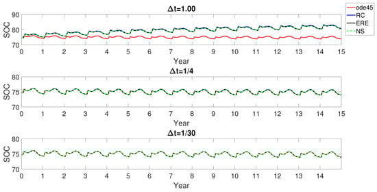
Figure 5. Long-term simulation of the SOC indicator over 15 years with the discrete RothC, ERE and NS methods. Stepsizes are set as $\Delta t=1$ (1 month), $\Delta t=1/4$ (1 week) and $\Delta t=1/30$ (1 day). The reference solution obtained by ode45 with tolerance at the machine precision is also plotted.

5. The Hoosfield Spring Barley Experiment

We illustrate the model and test the three methods using data from the Hoosfield spring barley experiment, one of the classical long-term experiments carried out at the Rothamster Experimental Station [22]. The same dataset was used as an example of the use of the RothC model in [6]. The Hoosfield experiment was conducted from 1852 till 2000. Spring barley has been grown continuously in the whole period, except in the years 1912, 1933, 1943 and 1967, when the experiment was fallowed to control weeds. The initial SOC content in the soil at 1852 was measured as $33.8632tC$ha${}^{-1}$, split out in the soil compartments in the following way: $2.7tC$ha${}^{-1}$ in IOM, $0.1533tC$ha${}^{-1}$ in DPM, $4.4852tC$ha${}^{-1}$ in RMP, $0.6671tC$ha${}^{-1}$ in BIO and $25.8576tC$ha${}^{-1}$ in HUM.

The $\rho$ function was estimated on a monthly basis from the weather dataset in [6], including average monthly air temperature, monthly open pan evaporation and monthly rainfall. It was also affected by the percentage of clay in the soil (23.4% in Rothamsted soil) and by the monthly soil cover factor (covered or fallow). Assuming that the soil was covered only from April to July for each crop year, the $\rho$ function assumed the values in Table 2. The other parameters of the model were set as $\alpha =0.10$, $\beta =0.12$, $\gamma =0.59$ and $\eta =0.49$. Moreover, the monthly decomposition rate vector $\mathbf{k}=[0.8333,0.0250,0.0550,0.0017]$ was considered.

Table 2. Monthly values for $\rho$ for the Hoosfield spring barley experiment, estimated from weather data in [6], clay content of 23.4% and soil cover factors in crop and fallow years.

	Jan.	Feb.	Mar.	Apr.	May	Jun.	July	Aug.	Sep.	Oct.	Nov.	Dec.
$\rho \left(t_n\right)$ Crop years	0.3561	0.3723	0.5068	0.4471	0.7473	0.7779	0.2491	0.4151	0.6570	1.1277	0.6092	0.4594
$\rho \left(t_n\right)$ Fallow years	0.3561	0.3723	0.5068	0.7451	1.2454	1.2965	0.4151	0.4151	0.6570	1.1277	0.6092	0.4594

Three different scenarios were simulated with the three numerical methods analysed in Section 3, and the results were compared with direct observations of SOC quantity in the soil in 1882, 1913, 1946, 1975, 1982 and 1987:

Scenario 1.

Unmanured treatment: For this scenario, the annual input of plant residuals was calculated to be $1.60tC$ha${}^{-1}$y${}^{-1}$, distributed as in Figure 6, in every year except in those that were fallow. For these years, a null plant residuals input was considered. In this scenario, FYM input was zero.

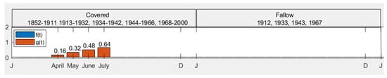Figure 6. Hoosfield barley experiment. Scenario 1: unmanured treatment.

Scenario 2.

Farmyard manure: The second treatment included inputs from both plant residuals and FYM, as scheduled in Figure 7. The annual input of plant residuals was calculated to be $2.8tC$ha${}^{-1}$y${}^{-1}$, greater than the one in Scenario 1, due to the farmyard treatment.

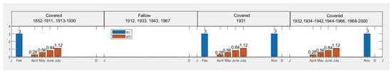Figure 7. Hoosfield barley experiment. Scenario 2: farmyard manure annually (two times in 1931).

Scenario 3.

Mixed treatment, farmyard manure till 1871: In this scenario, farmyard manure was assured every February till 1871 and nothing thereafter. This caused an annual plant residual input equal to $2.8tC$ha${}^{-1}$y${}^{-1}$ from 1852 till 1876 and equal to $1.60tC$ha${}^{-1}$y${}^{-1}$ in the following years, except for the fallow ones. Input data are shown in Figure 8.

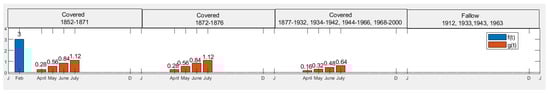Figure 8. Hoosfield barley experiment. Scenario 3: farmyard manure 1852–1871 and nothing thereafter.

Figure 9, Figure 10 and Figure 11 show the modelled data for total soil organic C in the three treatments, together with the measured data. The modelled results for Scenario 3 when the treatment considered FYM for only the first twenty years were considerably lower than the measurements; agreement was closer with the other two treatments (Scenarios 1 and 2). To test the models’ ability to predict the achievement of land degradation neutrality, note that all the simulations gave results in agreement with measured data, i.e., the loss of neutrality in 2000 for Scenario 1 and the achievement of neutrality for Scenario 2 with respect to the initial value in 1852. Measurements indicated the achievement of land degradation neutrality also for Scenario 3; in this case, however, the three models failed in predicting for $SOC\left(2000\right)$ a value lower than the initial one, i.e., $SOC\left(1852\right)=33.80tC\mathrm{h}{a}^{-1}$.

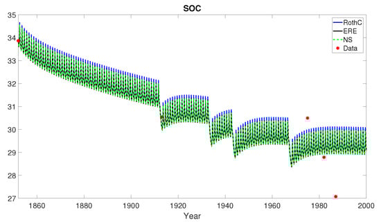
Figure 9. Hoosfield barley experiment. Scenario 1: unmanured treatment. Organic C in soil data (red bullets) modelled by the RothC (8), ERE (13) and NS (17) methods in the temporal horizon $[1852,2000]$ with $\Delta t=1$. According to Table 3, ERE approximation shows the best performance with respects to both the statistical indicators RMSE and modelling Efficiency (EF).

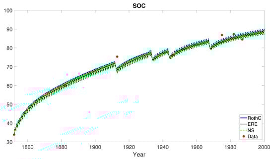
Figure 10. Hoosfield barley experiment. Scenario 2: farmyard manure annually. Organic C in soil data (red bullets) modelled by the RothC (8), ERE (13) and NS (17) methods in the temporal horizon $[1852,2000]$ with $\Delta t=1$. According to Table 3, RothC approximation shows the best performance with respect to both the statistical indicators RMSE and EF.

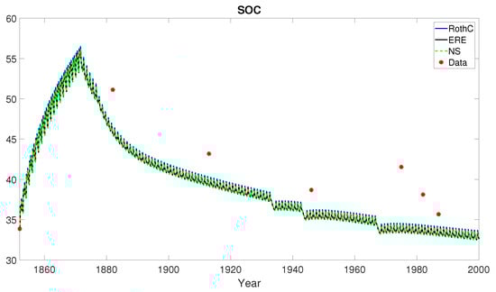
Figure 11. Hoosfield barley experiment. Scenario 3: farmyard manure 1852–1871 and nothing thereafter. Organic C in soil data (red bullets) modelled by the RothC (8), ERE (13) and NS (17) methods in the temporal horizon $[1852,2000]$ with $\Delta t=1$. According to Table 3, RothC approximation shows the best performance with respect to both the statistical indicators RMSE and EF.

To assess the performance of the discrete models and compare measured and simulated valued, as in [16], we used two well-known statistical indices: RMSE (Root Mean Squared Error) and EF (modelling Efficiency):

$$RMSE=\sqrt{{\displaystyle \frac{1}{N}}\sum _{i=1}^N{\left(O_i-S_i\right)}^2}EF=1-{\displaystyle \frac{{\displaystyle \sum _{i=1}^N{\left(O_i-S_i\right)}^2}}{{\displaystyle \sum _{i=1}^N{\left(O_i-\overline{O}\right)}^2}}}$$

where $O_i$ and $S_i$ are observed and simulated SOC at the ith value, $\overline{O}$ is the mean of the observed data and N is the number of observations. The closer the RMSE is to zero, the better the simulated solution describes the data. EF can range from $-\infty$ to one, with the best performance at EF = 1. Negative values of EF indicate that the observed mean is a better predictor than the model.

The results of the evaluation of the above indicators related to the three discrete models applied to approximate Hoosfield barley experiments data for the three different scenarios are reported in Table 3. The obtained values confirm that Scenario 3 was the worst case, i.e., the case when simulated data were more different from the measurements. The three discrete models provided similar values for the simulation of the three different treatments, and we could not select a method that clearly outperformed the others. However, from Table 3, we could set the ERE model as the best model for Scenario 1, while the RothC model provided better results for both Scenarios 2 and 3. Comparing the indicators for all scenarios with respect to the approximation of the experimental data, the minimum value of $RMSE=1.1596$ was assumed by the ERE model in Scenario 1, while the maximum value of $EF=0.9609$ was assumed by the RothC method in Scenario 2.

Table 3. RMSE and EF statistical indices for evaluating and comparing the performances of the RothC, ERE and novel non-standard NS models.

		Scenario 1			Scenario 2			Scenario 3
	RothC	ERE	NS	RothC	ERE	NS	RothC	ERE	NS
RMSE	1.1665	1.1596	1.1599	3.5406	3.6029	3.5961	4.5772	4.6310	4.6254
EF	0.7318	0.7350	0.7348	0.9609	0.9595	0.9597	0.2564	0.2388	0.2406

6. Conclusions

Soil organic carbon is one of the key indicators of land degradation status. In this paper, we analysed the RothC model, a simple tool developed for predicting the dynamic evolution of the content of soil organic carbon under the effect of weather conditions and land use data. Both the continuous version, based on a linear, non-autonomous differential system, and the original discrete monthly time-stepping procedure were considered. The aim of our study was to compare the qualitative analysis of both continuous and discrete dynamics in approximating steady-state and long-term periodic solutions. We focused on these aspects since they provide the information concerning the possible achievement of land degradation neutrality. We found that the steady-state solutions of the original discrete model were first-order accurate approximations of the steady-state solutions of the continuous differential model. The accuracy of the approximation represents the main weakness of the RothC discrete model when considered as a first-order accurate approximation of its continuous version. We point out that well-established numerical procedures such as, for example, the Exponential Rosenbrock–Euler (ERE) method, have, by construction, the same equilibria of the approximating differential system. Conversely, the discrete RothC model overestimates the steady-state equilibrium of the continuous flow, so that, in order to obtain the correct estimate with first-order accuracy, we have to reduce the stepsize of the updating time procedure. This fact may have a negative effect in real applications. It is necessary to run the RothC model to equilibrium first, in order to align the initial content of soil organic carbon with the measured one [6]. Nevertheless, the good matching of real data and numerical approximations, together with the available implementation in the RothC 26.3 open-source interface [6], justifies the wide use in the literature of the original discrete RothC model and explains the lack of use of more accurate numerical integrators. For this reason, in this paper, our additional objective was to propose a novel non-standard first-order procedure, the so-called NS discrete model, able to approximate the decomposition dynamics in the same way as the original discrete RothC model. This procedure features the same steady-state solution of the continuous model and exhibits a computational cost lower than the one required by the ERE time-stepping procedure. We also provided a simple code that implements both the original discrete RothC model and the monthly time-stepping NS and ERE models in a MATLAB environment. That allows the reproduction of our results and facilitates future comparisons among all the approaches. The discrete models were firstly tested on a hypothetical example as first-order accurate numerical integrators, and secondly, they were tested on the classical Hoosfield barley experiment to evaluate their ability in reproducing observed data. If we consider the discrete RothC model as a difference scheme, which approximates the continuous RothC differential system, numerical tests showed its coarseness with respect to both the ERE and NS procedures. When applied to the Hoosfield barley experiment, the three discrete models provided very similar results. However, the evaluation of the statistical error indicators still revealed the discrete RothC model as the best scheme for approximating real data in both Scenarios 2 and 3, while the ERE model outperformed the discrete RothC and the novel procedure in Scenario 1. In predicting the long-term behaviours, which are useful to establish the achievement of land degradation neutrality, the three discrete models failed in giving results in accordance with theoretical values in our hypothetical test, as well as with real data in the case of Scenario 3 of the Hoosfield spring barley experiment. This motivates our future research to consider more complex SOC dynamics. In particular, we will analyse the MOMOS model [23,24], which puts the microbial community at the centre of all transformation processes in the cycle of organic matter, from assimilation by degradation to loss by mineralization. Further analysis will also consider nonlinear SOC dynamics [25,26] and spatially explicit models described by partial differential equations [27,28] in order to deal with real domains, as protected areas, covered by non-homogeneous land use patterns. Finally, using field measurements and remote sensing information for modelling land degradation will significantly improve the obtained results [29]. The final aim is to select and provide a robust modelling tool for evaluating the trends of SOC stocks in the Alta Murgia National Park, where the achievement of land degradation neutrality is hampered by a combination of anthropic pressures and climate change [30,31,32].

References

- Orr, B.; Cowie, A.; Castillo Sanchez, V.; Chasek, P.; Crossman, N.; Erlewein, A.; Louwagie, G.; Maron, M.; Metternicht, G.; Minelli, S.; et al. Scientific conceptual framework for land degradation neutrality. In A Report of the Science-Policy Interface; United Nations Convention to Combat Desertification (UNCCD): Bonn, Germany, 2017. [Google Scholar]
- Aynekulu, E.; Lohbeck, M.; Nijbroek, R.P.; Ordoñez, J.C.; Turner, K.G.; Vågen, T.G.; Winowiecki, L.A. Review of Methodologies for Land Degradation Neutrality Baselines: Sub-National Case Studies from Costa Rica and Namibia; International Center for Tropical Agriculture (CIAT): Kampala, Uganda, 2017; 59p. [Google Scholar]
- FAO. Measuring and modelling soil carbon stocks and stock changes in livestock production systems: Guidelines for assessment (Version 1). In Livestock Environmental Assessment and Performance (LEAP) Partnership; FAO: Rome, Italy, 2019; p. 170. [Google Scholar]
- Paustian, K.; Collier, S.; Baldock, J.; Burgess, R.; Creque, J.; DeLonge, M.; Dungait, J.; Ellert, B.; Frank, S.; Goddard, T.; et al. Quantifying carbon for agricultural soil management: From the current status toward a global soil information system. Carbon Manag. 2019, 10, 567–587. [Google Scholar] [CrossRef]
- Ponce-Hernandez, R.; Koohafkan, P.; Antoine, J. Assessing Carbon Stocks and Modelling Win-Win Scenarios of Carbon Sequestration through Land-Use Changes; Food & Agriculture Org.: Rome, Italy, 2004; Volume 1. [Google Scholar]
- Coleman, K.; Jenkinson, D.S. ROTHC-26.3: A Model for the Turnover of Carbon in Soil: Model Description and Users Guide: K. Coleman and DS Jenkinson; IACR: Lyon, France, 1995. [Google Scholar]
- Parton, W. The CENTURY model. In Evaluation of Soil Organic Matter Models; Springer: Berlin/Heidelberg, Germany, 1996; pp. 283–291. [Google Scholar]
- Sallih, Z.; Pansu, M. Modelling of soil carbon forms after organic amendment under controlled conditions. Soil Biol. Biochem. 1993, 25, 1755–1762. [Google Scholar] [CrossRef]
- Martin, M.P.; Cordier, S.; Balesdent, J.; Arrouays, D. Periodic solutions for soil carbon dynamics equilibriums with time-varying forcing variables. Ecol. Model. 2007, 204, 523–530. [Google Scholar] [CrossRef][Green Version]
- Parshotam, A. The Rothamsted soil-carbon turnover model—Discrete to continuous form. Ecol. Model. 1996, 86, 283–289. [Google Scholar] [CrossRef]
- Coleman, K.; Jenkinson, D.; Crocker, G.; Grace, P.; Klir, J.; Körschens, M.; Poulton, P.; Richter, D. Simulating trends in soil organic carbon in long-term experiments using RothC-26.3. Geoderma 1997, 81, 29–44. [Google Scholar] [CrossRef]
- Morais, T.G.; Teixeira, R.F.; Domingos, T. Detailed global modelling of soil organic carbon in cropland, grassland and forest soils. PLoS ONE 2019, 14, e0222604. [Google Scholar] [CrossRef]
- Formaggia, L.; Scotti, A. Positivity and conservation properties of some integration schemes for mass action kinetics. SIAM J. Numer. Anal. 2011, 49, 1267–1288. [Google Scholar] [CrossRef]
- Martiradonna, A.; Colonna, G.; Diele, F. GeCo: Geometric Conservative non-standard schemes for biochemical systems. Appl. Numer. Math. 2020, 155, 38–57. [Google Scholar] [CrossRef]
- Diele, F.; Marangi, C. Geometric Numerical Integration in Ecological Modelling. Mathematics 2020, 8, 25. [Google Scholar] [CrossRef]
- Francaviglia, R.; Baffi, C.; Nassisi, A.; Cassinari, C.; Farina, R. Use of the “ROTHC” model to simulate soil organic carbon dynamics on a silty-loam inceptisol in Northern Italy under different fertilization practices. EQA-Int. J. Environ. Qual. 2013, 11, 17–28. [Google Scholar] [CrossRef]
- Farina, R.; Coleman, K.; Whitmore, A.P. Modification of the RothC model for simulations of soil organic C dynamics in dryland regions. Geoderma 2013, 200, 18–30. [Google Scholar] [CrossRef]
- Chen, Y.J.; Ascher, U.M.; Pai, D.K. Exponential Rosenbrock–Euler integrators for elastodynamic simulation. IEEE Trans. Vis. Comput. Graph. 2017, 24, 2702–2713. [Google Scholar] [CrossRef]
- Hochbruck, M.; Ostermann, A.; Schweitzer, J. Exponential Rosenbrock-type methods. SIAM J. Numer. Anal. 2009, 47, 786–803. [Google Scholar] [CrossRef]
- Mickens, R.E. Applications of Nonstandard Finite Difference Schemes; World Scientific: Singapore, 2000. [Google Scholar]
- Martiradonna, A. NSRothC-NonStandard RothC Models in Matlab. 2021. Available online: https://github.com/CnrIacBaGit/NSRothC (accessed on 8 February 2021).
- Rothamsted Experimental Station, Great Britain. Rothamsted: Guide to the Classical Field Experiments; AFRC Institute of Arable Crops Research: Hertsfordshire, UK, 1991. [Google Scholar]
- Pansu, M.; Sarmiento, L.; Rujano, M.; Ablan, M.; Acevedo, D.; Bottner, P. Modeling organic transformations by microorganisms of soils in six contrasting ecosystems: Validation of the MOMOS model. Glob. Biogeochem. Cycles 2010, 24, GB1008. [Google Scholar] [CrossRef]
- Pansu, M.; Machado, D.; Bottner, P.; Sarmiento, L. Modelling microbial exchanges between forms of soil nitrogen in contrasting ecosystems. Biogeosci. Discuss. 2014, 11, 915–927. [Google Scholar] [CrossRef]
- Hammoudi, A.; Iosifescu, O.; Bernoux, M. Mathematical analysis of a nonlinear model of soil carbon dynamics. Differ. Equ. Dyn. Syst. 2015, 23, 453–466. [Google Scholar] [CrossRef]
- Wang, Y.; Chen, B.; Wieder, W.R.; Leite, M.; Medlyn, B.E.; Rasmussen, M.; Smith, M.J.; Agusto, F.B.; Hoffman, F.; Luo, Y. Oscillatory behaviour of two nonlinear microbial models of soil carbon decomposition. Biogeosciences 2014, 11, 1817–1831. [Google Scholar] [CrossRef]
- Hammoudi, A.; Iosifescu, O. Mathematical Analysis of a Chemotaxis-Type Model of Soil Carbon Dynamic. Chin. Ann. Math. Ser. B 2018, 39, 253–280. [Google Scholar] [CrossRef]
- Elzein, A.; Balesdent, J. Mechanistic simulation of vertical distribution of carbon concentrations and residence times in soils. Soil Sci. Soc. Am. J. 1995, 59, 1328–1335. [Google Scholar] [CrossRef]
- Caspari, T.; van Lynden, G.; Bai, Z. Land Degradation Neutrality: An evaluation of methods. In Report Commissioned by German Federal Environment Agency (UBA); Umweltbundesamt: Dessau-Roßlau, Germany, 2015. [Google Scholar]
- Marangi, C.; Casella, F.; Diele, F.; Lacitignola, D.; Martiradonna, A.; Provenzale, A.; Ragni, S. Mathematical tools for controlling invasive species in Protected Areas. In Mathematical Approach to Climate Change and its Impacts; Springer: Berlin/Heidelberg, Germany, 2020; pp. 211–237. [Google Scholar]
- Lacitignola, D.; Diele, F.; Marangi, C. Dynamical scenarios from a two-patch predator–prey system with human control–Implications for the conservation of the wolf in the Alta Murgia National Park. Ecol. Model. 2015, 316, 28–40. [Google Scholar] [CrossRef]
- Baker, C.M.; Diele, F.; Lacitignola, D.; Marangi, C.; Martiradonna, A. Optimal control of invasive species through a dynamical systems approach. Nonlinear Anal. Real World Appl. 2019, 49, 45–70. [Google Scholar] [CrossRef]
Publisher’s Note: MDPI stays neutral with regard to jurisdictional claims in published maps and institutional affiliations. |
© 2021 by the authors. Licensee MDPI, Basel, Switzerland. This article is an open access article distributed under the terms and conditions of the Creative Commons Attribution (CC BY) license (https://creativecommons.org/licenses/by/4.0/).