An Inertial Generalized Viscosity Approximation Method for Solving Multiple-Sets Split Feasibility Problems and Common Fixed Point of Strictly Pseudo-Nonspreading Mappings

Abstract

In this paper, we propose a generalized viscosity iterative algorithm which includes a sequence of contractions and a self adaptive step size for approximating a common solution of a multiple-set split feasibility problem and fixed point problem for countable families of k-strictly pseudononspeading mappings in the framework of real Hilbert spaces. The advantage of the step size introduced in our algorithm is that it does not require the computation of the Lipschitz constant of the gradient operator which is very difficult in practice. We also introduce an inertial process version of the generalize viscosity approximation method with self adaptive step size. We prove strong convergence results for the sequences generated by the algorithms for solving the aforementioned problems and present some numerical examples to show the efficiency and accuracy of our algorithm. The results presented in this paper extends and complements many recent results in the literature.

1. Introduction

The problem of finding a point in the intersection of closed and convex subsets in real Hilbert spaces has appeared severally in diverse areas of mathematics and physical sciences. This problem is commonly referred to as the Convex Feasibility Problem (shortly, CFP), and finds its applications in various disciplines such as image restoration, computer tomograph and radiation therapy treatment planning, see [1]. A generalization of the CFP is the Split Feasibility Problem (SFP) which was introduced by Censor and Elfving [2] and defined as finding a point in a nonempty closed convex set, whose image under a bounded operator is in another set. Mathematically, the SFP can be formulated as:

$$\begin{array}{c}\hfill \mathrm{find}{x}^{*}\in C\mathrm{such}\mathrm{that}A{x}^{*}\in Q,\end{array}$$

(1)

where C and Q are nonempty closed convex subsets of ${\mathbb{R}}^N$ and ${\mathbb{R}}^M$ respectively, and A is a given matrix of dimension $N\times M.$ The SFP also models inverse problems arising from phase retrieval and intensity modulated radiation therapy [2]. Censor et al. [3] further introduced another generalization of the CFP and SFP called the Multiple Set Split Feasibility Problem (MSSFP) which is formulated as

$$\begin{array}{c}\hfill \mathrm{find}{x}^{*}\in C:={\cap }_{i=1}^k{C}_i\mathrm{such}\mathrm{that}A{x}^{*}\in Q:={\cap }_{j=1}^t{Q}_j,\end{array}$$

(2)

where $k\ge 1$ and $r\ge 1$ are given integers, A is a given $M\times N$ real matrix with $A^{*}$ its transpose, ${\left\{C_i\right\}}_{i=1}^k$ and ${\left\{Q_j\right\}}_{j=1}^t$ are nonempty closed convex subsets of ${\mathbb{R}}^N$ and ${\mathbb{R}}^M,$ respectively. Observe that when $k=r=1,$ the MSSFP reduces to SFP (1). In this paper, we focus on the MSSFP in a unified framework. We denote the set of solutions of (2) by $\Omega$ and assume that $\Omega$ is consistent (i.e., nonempty). It is well known that the MSSFP is equivalent to the following minimization problem:

$$\begin{array}{c}\hfill min\left\{\frac{1}{2}\parallel x-P_C{\left(x\right)\parallel }^2+\frac{1}{2}\parallel Ax-P_Q\left(Ax\right){\parallel }^2\right\},\end{array}$$

(3)

where $P_C$ and $P_Q$ are the orthogonal projections onto C and Q respectively. For solving (3), Censor et al. [3] defined a proximity function $p\left(x\right)$ for measuring the distance of a point to all sets as follows:

$$\begin{array}{c}\hfill p\left(x\right):=\frac{1}{2}{\displaystyle {\displaystyle \sum _{i=1}^k}}{\alpha }_i\parallel x-P_{C_i}{\left(x\right)\parallel }^2+\frac{1}{2}{\displaystyle {\displaystyle \sum _{j=1}^t}}{\beta }_j\parallel Ax-P_{Q_j}\left(Ax\right){\parallel }^2\end{array}$$

(4)

where ${\alpha }_i>0,{\beta }_j>0$$\forall i$ and j respectively, and ${\sum }_{i=1}^k{\alpha }_i+{\sum }_{j=1}^t{\beta }_j=1.$ It is easy to see that

$$\begin{array}{c}\hfill ▽p\left(x\right):={\displaystyle {\displaystyle \sum _{i=1}^k}}{\alpha }_i(x-P_{C_i}\left(x\right))+{\displaystyle {\displaystyle \sum _{j=1}^t}}{\beta }_j{A}^{*}(I-P_Q)Ax.\end{array}$$

Censor et al. [3] also introduced the following projection method for solving the MSSFP:

$$\begin{array}{c}\hfill x_{n+1}=P_{\Omega }(x_n-s▽p\left(x_n\right)),\end{array}$$

(5)

where s is a positive scalar. They further proved the weak convergence of (5) under the condition that the stepsize s satisfies

$$0<s_L\le s\le s_{\mu }<\frac{2}{L},$$

where $L={\sum }_{i=1}^k{\alpha }_i+\rho \left(A^{*}A\right){\sum }_{j=1}^t{\beta }_j$ is the Lipschitz constant of $▽p$. A major setback of (5) is the fact that the algorithm used a fixed stepsize which is restricted by the Lipschitz constant (this depends on the largest eigenvalue of the matrix $A^{*}A$). Computing the largest eigenvalue of $A^{*}A$ is usually difficult and its conservation results in slow convergence. More so, note that the projection onto the sets C and Q are often difficult to calculate when the sets are not simple. This can also result in the complication of (5). Several efforts have been made in order to find best appropriate modifications of (5) without the setbacks in infinite dimensional real Hilbert spaces. For instance, Zhao and Yang [4] introduced a new projection method such that the stepsize s is selected via an Armijo line search technique for solving the MSSFP. However, this line search process required extra inner iteration for obtaining a suitable stepsize. The authors in [5] also introduced a self-adaptive projection method which requires the computation of the stepsize directly without any inner iteration. More so, López et al. [6] introduced a relaxed projection method with a fixed stepsize and proved a weak convergence result for solving the MSSFP. He et al. [7] further combined a Halpern iterative scheme with the relaxed projection method and proved a strong convergence result for solving the MSSFP. Recently, Suantai et al. [8] introduced an inertial relaxed projection method with a self-adaptive stepsize for solving the MSSFP. Also, Wen et al. [9] introduced a cyclic-simultaneous projection method and proved weak convergence result for solving the MSSFP.

Constructing iterative schemes with a faster rate of convergence are usually of great interest. The inertial-type algorithm which originated from the equation for an oscillator with damping and conservative restoring force has been an important tool employed in improving the performance of algorithms and has some nice convergence characteristics. In general, the main feature of the inertial-type algorithms is that we can use the previous iterates to construct the next one. Since the introduction of the inertial-like algorithm, many authors combined the inertial term $\left[{\theta }_n(x_n-x_{n-1})\right]$ together with different kinds of iterative algorithms, including Mann, Kranoselski, Halpern, Viscosity, to mention a few, to approximate solutions of fixed point problems and optimization problems. Most authors were able to prove weak convergence results while few proved strong convergence results.

Polyak [10] was the first author to propose the heavy ball method, Alvarez and Attouch [11] employed this to the setting of a general maximal monotone operator using the Proximal Point Algorithm (PPA), which is called the inertial PPA, and is of the form:

$$\begin{array}{c}\hfill \left\{\begin{array}{c}{y}_n=x_n+{\theta }_n(x_n-x_{n-1}),\hfill \\ x_{n+1}={(I+r_{n}B)}^{-1}{y}_n,n>1.\hfill \end{array}\right.\end{array}$$

(6)

They proved that if $\left\{r_n\right\}$ is non-decreasing and $\left\{{\theta }_n\right\}\subset [0,1)$ with

$$\begin{array}{c}\hfill {\displaystyle {\displaystyle \sum _{n=1}^{+\infty }}}{\theta }_n\parallel x_n-x_{n-1}{\parallel }^2<+\infty ,\end{array}$$

(7)

then the Algorithm (6) converges weakly to a zero of a maximal monotone operator B. More precisely, condition (7) is true for ${\theta }_n<\frac{1}{3}$. Here ${\theta }_n$ is an extrapolation factor. Other initial-type algorithms can be found in, for instance [12,13,14,15,16,17].

Motivated by the works of Wen et al. [9] and López et al. [6], in this paper, we introduce a general viscosity relaxed projection method with inertial process for solving the MSSFP with the fixed point of strictly pseudo-nonspreading mappings in real Hilbert spaces. The stepsize of our algorithm is selected self-adaptively in each iteration and its convergence does not involve prior estimate of the matrix $A^{*}A.$ More so, we define some sublevel sets whose projections can be calculated explicitly using the formula in [18]. The general viscosity approximation method guarantees strong convergence of the sequences generated by the algorithm. This improves the weak convergence results proved in [6,9,19]. We further provide some numerical experiments to illustrate the performance and accuracy of our algorithm. Our results improve and complement the results of [6,7,8,9,19,20,21,22,23,24] and many other results in this direction.

2. Preliminaries

We state some known and useful results which will be needed in the proof of our main theorem. In the sequel, we denote strong and weak convergence by “→” and “⇀”, respectively.

Let C be a nonempty closed convex subset of a real Hilbert space H with inner product $\langle .,.\rangle$ and norm $\left|\right|.\left|\right|$. Let $S:C\to C$ be a nonlinear mapping and $F\left(S\right)=\{x\in C:Sx=x\}$ be the set of all fixed points of S.

A mapping $S:C\to C$ is called

• nonexpansive, if

  $$\begin{array}{c}\hfill \parallel Sx-Sy\parallel \le \parallel x-y\parallel ,\forall x,y\in C;\end{array}$$
• quasi-nonexpansive, if $F\left(S\right)$ is nonempty, and

  $$\begin{array}{c}\hfill \parallel Sx-p\parallel \le \parallel x-p\parallel ,\forall p\in F\left(S\right);\end{array}$$
• nonspreading [25], if

  $$\begin{array}{c}\hfill 2\parallel Sx-{Sy\parallel }^2\le \parallel Sx-{y\parallel }^2+\parallel Sy-{x\parallel }^2,\forall x,y\in C;\end{array}$$
• k-strictly pseudo-nonspreading in terms of Browder-Petryshyn [26], if there exists $k\in [0,1)$ such that

  $$\begin{array}{c}\hfill \parallel Sx-{y\parallel }^2\le \parallel x-{y\parallel }^2+k\parallel x-Sx-{(y-Sy)\parallel }^2+2\langle x-Sx,y-Sy\rangle ,\forall x.y\in C.\end{array}$$

Remark 1.

(a) 

If $S:C\to C$ is a nonspreading mapping with $F\left(S\right)\ne \varnothing$, then S is quasi-nonexpansive and $F\left(S\right)$ is closed and convex.

(b) 

It is also clear that every nonspreading mapping is k-strictly pseudo-nonspreading with k=0, but the converse is not true, see example 3 in [27].

Lemma 1.

[27] Let $T:C\to C$ be a k-strictly pseudo-nonspreading mapping with $k\in [0,1)$. Denote $T_{\beta }:=\beta I+(1-\beta )T$, where $\beta \in [k,1)$, then

(a) 

$F\left(T\right)=F\left(T_{\beta }\right),$

(b) 

the following inequality holds:

$$\begin{array}{c}\hfill \parallel T_{\beta }x-T_{\beta }{y\parallel }^2\le \parallel x-{y\parallel }^2+\frac{2}{1-\beta }\langle x-T_{\beta }x,y-T_{\beta }y\rangle ,\forall x,y\in C;\end{array}$$

(c) 

$T_{\beta }$ is a quasi-nonexpansive mapping.

Lemma 2.

[28] Let $C\subset H$ be nonempty, closed and convex set. Then, $\forall x,y\in H$ and $z\in C$

1. 

$\langle x-P_{C}x,z-P_{C}x\rangle \le 0,$

2. 

$\parallel P_{C}x-P_{C}y{\parallel }^2\le \langle P_{C}x-P_{C}y,x-y\rangle ,$

3. 

$\parallel P_{C}x-{z\parallel }^2\le \parallel x-{z\parallel }^2-\parallel P_{C}x-x{\parallel }^2.$

Lemma 3.

[29] Let H be a real Hilbert space and ${\left\{x_i\right\}}_{i\ge 1}$ be a bounded sequence in H. For ${\alpha }_i\in (0,1)$ such that ${\sum }_{i=1}^{\infty }{\alpha }_i=1$, the following identity holds

$$\begin{array}{c}\hfill \parallel {\displaystyle {\displaystyle \sum _{i=1}^{\infty }}}{\alpha }_i{x}_i{\parallel }^2={\displaystyle {\displaystyle \sum _{i=1}^{\infty }}}{\alpha }_i\parallel x_i{\parallel }^2-{\displaystyle {\displaystyle \sum _{1\le i<j<\infty }}}{\alpha }_i{\alpha }_j\parallel x_i-x_j{\parallel }^2.\end{array}$$

More so, from Lemma 3, we get the following result.

Lemma 4.

[30] For all $x_1,x_2,\dots ,x_n\in H,$ the following inequality holds:

$$\begin{array}{c}\hfill \parallel {\displaystyle {\displaystyle \sum _{i=1}^n}}{\lambda }_i{x}_i{\parallel }^2={\displaystyle {\displaystyle \sum _{i=1}^n}}{\lambda }_i\parallel x_i{\parallel }^2-\frac{1}{2}{\displaystyle {\displaystyle \sum _{i,j=1}^n}}{\lambda }_i{\lambda }_j\parallel x_i-x_j{\parallel }^2,n\ge 2,\end{array}$$

where ${\lambda }_i\in [0,1],i=1,2,\dots ,n,{\sum }_{i=1}^n{\lambda }_i=1.$

Lemma 5.

[27] Let C be a closed convex subset of H,  $T:C\to C$ be a k-strictly pseudo-nonspreading mapping with $F\left(T\right)\ne \varnothing$. If $\left\{x_n\right\}$ is a sequence in C which converges weakly to p and $\left\{(I-T)x_n\right\}$ converges strongly to q, then $(I-T)p=q$. In particular, if $q=0$, then $p=Tp$.

Lemma 6.

[31] Let $\left\{a_n\right\}$ be a sequence of nonegative real numbers $\left\{{\gamma }_n\right\}$ be a sequence of real numbers in $(0,1)$ with conditions ${\sum }_{n=1}^{\infty }{\gamma }_n=\infty$ and $\left\{d_n\right\}$ be a sequence of real numbers. Assume that

$$\begin{array}{c}\hfill a_{n+1}\le (1-{\gamma }_n)a_n+{\gamma }_n{d}_n,n\ge 1.\end{array}$$

If ${lim\; sup}_{k\to \infty }{d}_{n_k}\le 0$ for every subsequence $\left\{a_{n_k}\right\}$ of $\left\{a_n\right\}$ satisfying the condition:

${lim\; inf}_{k\to \infty }(a_{n_{k+1}}-a_{n_k})\ge 0,then{lim}_{n\to \infty }{a}_n=0.$

3. Main Results

In this section, we present our iterative algorithm and its convergence result.

Let $H_1$ and $H_2$ be real Hilbert spaces, C be a nonempty, closed and convex subset of a real Hilbert space H and $\left\{g_n\right\}$ be a sequence of $\left\{{\sigma }_n\right\}$-contractive self maps of H with ${lim\; inf}_{n\to \infty }{\sigma }_n\le {lim\; sup}_{n\to \infty }{\sigma }_n={\sigma }_{\mu }<1.$ Suppose that $\left\{g_n\left(x\right)\right\}$ is uniformly convergent to $\left\{g\right(x\left)\right\}$ for any $x\in D,$ where D is a bounded subset of C, let $S_m:H_1\to H_1,$ be a countable family of $k_m$-strictly pseudo-nonspreading mapping with $k:={sup}_{m\ge 1}{k}_m\in (0,1)$ and $S_{m,\beta }:=\beta I+(1-\beta )S_m,$ where $\beta \in [k,1),$ and $m\in \mathbb{N}\backslash \left\{0\right\}.$

Before we state our algorithm, we assume that the following conditions hold:

(A1)

The set $C_i$ is given by $C_i=\{x\in H_1:c_i\left(x\right)\le 0\}$ where $c_i:H_1\to \mathbb{R}$ $(i=1,2\dots ,k)$ are convex functions. Also, the set $Q_j$ is given by $Q_j=\{y\in H_2:q_j\left(y\right)\le 0\}$ $(j=1,2,\dots ,t)$ are convex functions. In addition, we assume that both $c_i$ and $q_j$ are subdifferentiable on $H_1$ and $H_2$ respectively and $\partial c_i$ and $\partial q_j$ are bounded operators.

(A2)

For any $x\in H_1$ and $y\in H_2,$ at least one subgradient ${\xi }_i\in \partial c_i\left(x\right)$ and ${\eta }_j\in \partial q_j\left(y\right)$ can be calculated, where $\partial c_i\left(x\right)$ and $\partial q_j\left(y\right)$ denote the subdifferentials of $c_i$ and $q_j$ at x and y respectively, i.e.,

$$\partial c_i\left(x\right)=\{{\xi }_i\in H_1:c_i\left(z\right)\ge c_i\left(x\right)+\langle {\xi }_i,z-x\rangle \forall z\in H_1\},$$

and

$$\partial q_j\left(y\right)=\{{\eta }_j\in H_2:q_j\left(u\right)\ge q_j\left(y\right)+\langle {\eta }_j,u-y\rangle \forall u\in H_2\}.$$

(A3)

We set $C_i^n$ and $Q_j^n$ as the half-spaces defined by

$$C_i^n=\{x\in H_1:c_i\left(x_n\right)+\langle {\xi }_i^n,x-x_n\rangle \le 0\},$$

where ${\xi }_n^n\in \partial c_i\left(x_n\right)$$(i=1,2,\dots ,k)$ and

$$Q_j^n=\{y\in H_2:q_j\left(A{x}_n\right)+\langle {\eta }_j^n,y-A{x}_n\rangle \le 0\},$$

where ${\eta }_j^n\in \partial q_j\left(A{x}_n\right)$$(j=1,2,\dots ,t).$

(A4)

We define the proximity function by

$$f_n\left(x\right)=\frac{1}{2}{\displaystyle \sum _{j=1}^t}{\lambda }_j\parallel Ax-P_{Q_j^n}\left(Ax\right){\parallel }^2,$$

where ${\lambda }_j>0$$\forall 1\le j\le t.$ Then the gradient of $f_n\left(x\right)$ is given by

$$\nabla f_n\left(x\right)={\displaystyle \sum _{j=1}^t}{\lambda }_j{A}^{*}(I-P_Q^n)\left(Ax\right).$$

(A5)

The control sequences $\left\{{\alpha }_n\right\},\left\{w_i\right\},\left\{{\gamma }_{n,m}\right\}$ and $\left\{{\rho }_n\right\}$ are chosen such that

-

$\left\{{\alpha }_n\right\}\subset (0,1),$${\displaystyle {\displaystyle \underset{n\to +\infty }{lim}}}{\alpha }_n=0,$${\displaystyle {\displaystyle \sum _{n=1}^{+\infty }}}{\alpha }_n=+\infty ;$

-

$\left\{{\gamma }_{n,m}\right\}\subset (0,1),$${\displaystyle {\displaystyle \underset{n\to +\infty }{lim\; inf}}}{\gamma }_{n,0}{\gamma }_{n,m}>0,$${\displaystyle {\displaystyle \sum _{m=0}^{+\infty }}}{\gamma }_{n,m}=1;$

-

$\left\{w_i\right\}\subseteq [0,1]$ with ${\displaystyle {\displaystyle \sum _{i=1}^{+\infty }}}{w}_i=1;$

-

$\left\{{\rho }_n\right\}\subset (0,4)$ and ${\displaystyle {\displaystyle \underset{n\to +\infty }{lim\; inf}}}{\rho }_n(4-{\rho }_n)>0.$

We now present our algorithm as follows:

First we show that the sequence $\left\{x_n\right\}$ generated by Algorithm 1 is bounded.

Algorithm 1: GVA

Step 0: Select the initial point $x_1\in H$ and the sequences $\left\{{\alpha }_n\right\},\left\{w_i\right\},\left\{{\gamma }_{n,m}\right\},\left\{{\rho }_n\right\}$ such that Assumption (A5) is satisfied. Set $n=1.$ Step 1: Given the nth iterate (i.e., $x_n,n\ge 0$), if $\nabla f_n\left(x_n\right)=0,$ STOP. Otherwise, compute $$y_n={\displaystyle \sum _{i=1}^k}{\omega }_i{P}_{C_i^n}(x_n-{\tau }_n\nabla f_n\left(x_n\right)),$$ where the stepsize ${\tau }_n$ is defined by $${\tau }_n=\frac{{\rho }_n{f}_n\left(x_n\right)}{\parallel \nabla f_n\left(x_n\right){\parallel }^2}.$$ Step 2: Compute $$x_{n+1}={\alpha }_n{g}_n\left(x_n\right)+(1-{\alpha }_n)\left({\gamma }_{n,0}{y}_n+{\displaystyle \sum _{m=1}^{\infty }}{\gamma }_{n,j}{S}_{m,\beta }{y}_n\right).$$ Step 3: Set $n\leftarrow n+1$ and return to Step 1.

Lemma 7.

Suppose the solution set $\Gamma =\left\{\Omega \cap {\bigcap }_{m=1}^{\infty }F\left(S_m\right)\right\}\ne \varnothing$ and $\left\{x_n\right\}$ is the sequence generated by Algorithm 1. Then $\left\{x_n\right\}$ is bounded.

Proof. 

Let $x^{*}\in \Gamma$ and $w_n={\gamma }_{n,0}{y}_n+{\sum }_{m=1}^{\infty }{\gamma }_{n,m}{S}_{m,\beta }{y}_n.$ By applying the nonexpansivity property of the projection mapping and Lemma 4, we have

$$\begin{array}{cc}\hfill \parallel y_n-x^{*}{\parallel }^2& =\parallel {\displaystyle \sum _{i=1}^k}{\omega }_i{P}_{C_i^n}(x_n-{\tau }_n\nabla f_n\left(x_n\right))-x^{*}{\parallel }^2\hfill \\ & \le \parallel x_n-{\tau }_n\nabla f_n\left(x_n\right)-x^{*}{\parallel }^2\hfill \\ & =\parallel x_n-x^{*}{\parallel }^2-2{\tau }_n\langle \nabla f_n\left(x_n\right),x_n-x^{*}\rangle +\parallel {\tau }_n\nabla f_n\left(x_n\right){\parallel }^2.\hfill \end{array}$$

(8)

Also from Lemma 2, we obtain

$$\begin{array}{cc}\hfill \langle \nabla f_n\left(x_n\right),x_n-x^{*}\rangle & =\langle {\displaystyle \sum _{j=1}^t}{\lambda }_j{A}^{*}(I-P_{Q_j^n})A{x}_n,x_n-x^{*}\rangle \hfill \\ & ={\displaystyle \sum _{j=1}^t}{\lambda }_j\langle (I-P_{Q_j^n})A{x}_n,A{x}_n-P_{Q_j^n}\left(A{x}_n\right)\rangle +{\displaystyle \sum _{j=1}^t}{\lambda }_j\langle (I-P_{Q_j^n})A{x}_n,P_{Q_j^n}\left(A{x}_n\right)-A{x}^{*}\rangle \hfill \\ & \ge {\displaystyle \sum _{j=1}^t}{\lambda }_j\parallel A{x}_n-P_{Q_j^n}\left(A{x}_n\right){\parallel }^2\hfill \\ & =2f_n\left(x_n\right).\hfill \end{array}$$

(9)

On substituting (9) into (8), we have

$$\begin{array}{cc}\hfill \parallel y_n-x^{*}{\parallel }^2& \le \parallel x_n-x^{*}{\parallel }^2-4{\tau }_n{f}_n\left(x_n\right)+\parallel {\tau }_n\nabla f_n\left(x_n\right){\parallel }^2\hfill \\ & =\parallel x_n-x^{*}{\parallel }^2-{\rho }_n(4-{\rho }_n)\frac{f_n^2\left(x_n\right)}{\parallel \nabla f_n\left(x_n\right){\parallel }^2}\hfill \\ & \le \parallel x_n-x^{*}{\parallel }^2.\hfill \end{array}$$

(10)

More so from Lemma 1, we get

$$\begin{array}{cc}\hfill \parallel w_n-x^{*}\parallel & =\parallel {\gamma }_{n,0}{y}_n+{\displaystyle \sum _{m=1}^{\infty }}{\gamma }_{n,m}{S}_{m,\beta }{y}_n-x^{*}\parallel \hfill \\ & \le {\gamma }_{n,0}\parallel y_n-x^{*}\parallel +{\displaystyle \sum _{m=1}^{\infty }}{\gamma }_{n,m}\parallel S_{m,\beta }{y}_n-x^{*}\parallel \hfill \\ & \le {\gamma }_{n,0}\parallel y_n-x^{*}\parallel +{\displaystyle \sum _{m=1}^{\infty }}{\gamma }_{n,m}\parallel y_n-x^{*}\parallel \hfill \\ & =\parallel y_n-x^{*}\parallel .\hfill \end{array}$$

(11)

Therefore from (10) and (11), we have

$$\begin{array}{cc}\hfill \parallel x_{n+1}-x^{*}\parallel & =\parallel {\alpha }_n{g}_n\left(x_n\right)+(1-{\alpha }_n)w_n-x^{*}\parallel \hfill \\ & \le {\alpha }_n\parallel g_n\left(x_n\right)-x^{*}\parallel +(1-{\alpha }_n)\parallel w_n-x^{*}\parallel \hfill \\ & \le {\alpha }_n{\sigma }_n\parallel x_n-x^{*}\parallel +(1-{\alpha }_n)\parallel x_n-x^{*}\parallel +{\alpha }_n\parallel g_n\left(x^{*}\right)-x^{*}\parallel \hfill \\ & \le (1-{\alpha }_n(1-{\sigma }_n))\parallel x_n-x^{*}\parallel +{\alpha }_n(1-{\sigma }_n)\frac{\parallel g_n\left(x^{*}\right)-x^{*}\parallel }{1-{\sigma }_n}\hfill \\ & ⋮\hfill \\ & \le max\left\{\parallel x_n-x^{*}\parallel ,\frac{\parallel g_n\left(x^{*}\right)-x^{*}\parallel }{1-{\sigma }_n}\right\}.\hfill \end{array}$$

Since $\left\{g_n\right\}$ is uniformly convergent on D, it follows that $\left\{g_n\left(x^{*}\right)\right\}$ is bounded. Thus, there exists a positive constant M, such that $\parallel g_n\left(x^{*}\right)-x^{*}\parallel \le M$. By induction, we obtain

$$\begin{array}{c}\hfill \parallel x_n-x^{*}\parallel \le max\left\{\parallel x_1-x^{*}\parallel ,\frac{M}{1-{\sigma }_{\mu }}\right\}.\end{array}$$

Hence, $\left\{x_n\right\}$ is bounded. Consequently $\left\{S_{m,\beta }{x}_n\right\},\left\{g_n\left(x_n\right)\right\},\left\{y_n\right\}$ and $\left\{w_n\right\}$ are all bounded. □

We now give our main convergence theorem.

Theorem 1.

Suppose that $\Gamma =\left\{\Omega \cap {\bigcap }_{m=1}^{\infty }F\left(S_m\right)\right\}\ne \varnothing$ and Assumptions (A1)–(A5) hold. Then, the sequence $\left\{x_n\right\}$ generated by Algorithm 1 converges strongly to point $z\in P_{\Gamma }$ which is a unique solution of the variational inequality

$$\begin{array}{c}\hfill \langle g\left(z\right)-z,x^{*}-z\rangle \le 0,\forall x^{*}\in P_{\Gamma }.\end{array}$$

Proof. 

From Lemma 1 (c), Lemma 3 and (10), we have

$$\begin{array}{cc}\hfill \parallel w_n-x^{*}{\parallel }^2& =\parallel {\gamma }_{n,0}{y}_n+{\displaystyle \sum _{m=1}^{\infty }}{\gamma }_{n,m}{S}_{m,\beta }{y}_n-x^{*}{\parallel }^2\hfill \\ & ={\gamma }_{n,0}\parallel y_n-x^{*}{\parallel }^2+{\displaystyle \sum _{m=1}^{\infty }}{\gamma }_{n,m}\parallel S_{m,\beta }{y}_n-x^{*}{\parallel }^2-{\displaystyle \sum _{m=1}^{\infty }}{\gamma }_{n,0}{\gamma }_{n,m}\parallel y_n-S_{m,\beta }{y}_n\parallel \hfill \\ & -{\displaystyle \sum _{1\le m<r<\infty }}{\gamma }_{n,m}{\gamma }_{n,r}\parallel S_{m,\beta }^m-S_{m,\beta }^r{\parallel }^2\hfill \\ & \le {\gamma }_{n,0}\parallel y_n-x^{*}{\parallel }^2+{\displaystyle \sum _{m=1}^{\infty }}{\gamma }_{n,m}\parallel y_n-x^{*}{\parallel }^2-{\displaystyle \sum _{m=1}^{\infty }}{\gamma }_{n,0}{\gamma }_{n,m}\parallel y_n-S_{m,\beta }{y}_n\parallel \hfill \\ & =\parallel y_n-x^{*}{\parallel }^2-{\displaystyle \sum _{m=1}^{\infty }}{\gamma }_{n,0}{\gamma }_{n,m}\parallel y_n-S_{m,\beta }{y}_n\parallel \hfill \\ & \le \parallel x_n-x^{*}{\parallel }^2-{\rho }_n(4-{\rho }_n)\frac{f_n^2\left(x_n\right)}{\parallel \nabla f_n\left(x_n\right){\parallel }^2}-{\displaystyle \sum _{m=1}^{\infty }}{\gamma }_{n,0}{\gamma }_{n,m}\parallel y_n-S_{m,\beta }{y}_n\parallel .\hfill \end{array}$$

(12)

Now, from (10) and (12), we have that

$$\begin{array}{cc}\hfill \parallel x_{n+1}-x^{*}{\parallel }^2& =\parallel {\alpha }_n{g}_n\left(x_n\right)+(1-{\alpha }_n)w_n-x^{*}{\parallel }^2\hfill \\ & \le {(1-{\alpha }_n)}^2\parallel w_n-x^{*}{\parallel }^2+2{\alpha }_n\langle x_{n+1}-x^{*},g_n\left(x_n\right)-x^{*}\rangle \hfill \\ & \le {(1-{\alpha }_n)}^2\parallel x_n-x^{*}{\parallel }^2-(1-{\alpha }_n){\rho }_n(4-{\rho }_n)\frac{f_n^2\left(x_n\right)}{\parallel \nabla f_n\left(x_n\right)\parallel }\hfill \\ & -(1-{\alpha }_n){\displaystyle \sum _{m=1}^{\infty }}{\gamma }_{n,0}{\gamma }_{n,m}\parallel y_n-S_{m,\beta }{y}_n\parallel +2{\alpha }_n\langle x_{n+1}-x^{*},g_n\left(x_n\right)-x^{*}\rangle \hfill \\ & ={(1-{\alpha }_n)}^2\parallel x_n-x^{*}{\parallel }^2+{\alpha }_n\left(2\langle x_{n+1}-x^{*},g_n\left(x_n\right)-x^{*}\rangle \right).\hfill \end{array}$$

(13)

Putting $d_n=2\langle x_{n+1}-x^{*},g_n\left(x_n\right)-x^{*}\rangle$, in view of Lemma 5, we need to prove that ${lim\; sup}_{k\to \infty }{d}_{n_k}\le 0$ for every $\left\{\right||x_{n_k}-x^{*}|\left|\right\}$ of $\left\{\right||x_n-x^{*}|\left|\right\}$ satisfying the condition

$$\begin{array}{c}\hfill {\displaystyle \underset{k\to +\infty }{lim\; inf}}\{\parallel x_{n_{k+1}}-x^{*}\parallel -\parallel x_{n_k}-x^{*}\parallel \}\ge 0.\end{array}$$

(14)

To show this, suppose that $\left\{\right||x_{n_k}-x^{*}|\left|\right\}$ is a subsequence of $\left\{\right||x_n-x^{*}|\left|\right\}$ such that (14) holds. Then

$$\begin{array}{cc}\hfill {\displaystyle \underset{k\to +\infty }{lim\; inf}}& (\parallel x_{n_{k+1}}-x^{*}|{|}^2-\parallel x_{n_k}-x\left|{|}^2\right)\hfill \\ & ={\displaystyle \underset{k\to \infty }{lim\; inf}}\left(\right(\parallel x_{n_{k+1}}-x^{*}{\parallel }^2-\parallel x_{n_k}-x^{*}{\parallel }^2\left)\right(\parallel x_{n_{k+1}}-x^{*}\parallel +\parallel x_{n_k}-x^{*}\parallel \left)\right)\ge 0.\hfill \end{array}$$

Now, using (12), we have that

$$\begin{array}{cc}\hfill {\displaystyle \underset{k\to +\infty }{lim\; sup}}((1-{\alpha }_{n_k}){\displaystyle \sum _{m=1}^{+\infty }}{\gamma }_{n_k,0}{\gamma }_{n_k,m}\parallel y_{n_k}-S_{m,\beta }{y}_{n_k}\parallel )& \le {\displaystyle \underset{k\to +\infty }{lim\; sup}}((1-{\alpha }_{n_k})\parallel x_{n_k}-x^{*}{\parallel }^2-\parallel x_{n_k+1}-x^{*}{\parallel }^2\hfill \\ & +2{\alpha }_{n_k}\langle x_{n_{k+1}}-x^{*},g_{n_k}\left(x_{n_k}\right)-x^{*}\rangle )\hfill \\ & \le {\displaystyle \underset{k\to +\infty }{lim\; sup}}(\parallel x_{n_k}-x^{*}{\parallel }^2-\parallel x_{n_k+1}-x^{*}{\parallel }^2)\hfill \\ & +{\displaystyle \underset{k\to +\infty }{lim\; sup}}\left(2{\alpha }_{n_k}\langle x_{n_k+1}-x^{*},g_{n_k}\left(x_{n_k}\right)-x^{*}\rangle \right)\hfill \\ & =-{\displaystyle \underset{k\to +\infty }{lim\; inf}}(\parallel x_{n_k+1}-x^{*}{\parallel }^2-\parallel x_{n_k}-x^{*}{\parallel }^2)\le 0.\hfill \end{array}$$

(15)

Hence

$$\begin{array}{c}\hfill {\displaystyle \underset{k\to +\infty }{lim}}\parallel y_{n_k}-S_{m,\beta }{y}_{n_k}\parallel =0.\end{array}$$

Please note that

$$\begin{array}{ccc}\hfill \parallel S_{m,\beta }{y}_n-y_n\parallel & =& \parallel \beta y_n+(1-\beta )S_m{y}_n-y_n\parallel \hfill \\ & =& (1-\beta )\parallel S_m{y}_n-y_n\parallel .\hfill \end{array}$$

Then it follows that

$$\parallel S_m{y}_n-y_n\parallel =\frac{1}{1-\beta }\parallel S_{m,\beta }{y}_n-y_n\parallel \to 0.$$

(16)

Furthermore, using (12) and following the same approach as in (15), we also have that

$$\begin{array}{c}\hfill {\rho }_n(4-{\rho }_n)\frac{f_n^2\left(x_{n_k}\right)}{\parallel ▽f\left(x_{n_k}\right){\parallel }^2}\le {\rho }_{n_k}(4-{\rho }_{n_k})\frac{f_n^2\left(x_{n_k}\right)}{\parallel ▽f\left(x_{n_k}\right){\parallel }^2}\to 0,\mathrm{as}k\to \infty .\end{array}$$

(17)

This implies that

$$\begin{array}{c}\hfill {\displaystyle \sum _{n=0}^{+\infty }}\frac{f_n^2\left(x_{n_k}\right)}{\parallel ▽f\left(x_{n_k}\right){\parallel }^2}<+\infty .\end{array}$$

(18)

Since $\nabla f_n$ is Lipschitz continuous and $\left\{x_n\right\}$ is bounded, so $\{\nabla f_n\left(x_n\right)\}$ is also bounded. Hence from (18), we can conclude that

$$\begin{array}{c}\hfill {\displaystyle \underset{k\to +\infty }{lim}}\frac{1}{2}{\displaystyle \sum _{j=1}^t}{\lambda }_j\parallel A{x}_{n_k}-P_{Q_j^n}\left(A{x}_{n_k}\right){\parallel }^2=0,\end{array}$$

(19)

which also implies that

$$\begin{array}{c}\hfill {\displaystyle \underset{k\to +\infty }{lim}}\parallel A{x}_{n_k}-P_{Q_j^n}\left(A{x}_{n_k}\right)\parallel =0,\mathrm{for}j=1,2,\dots ,t.\end{array}$$

(20)

Since $\partial q_j$ is bounded on bounded sets, there exists $\eta$ such that $\parallel {\eta }_j^n\parallel \le \eta$$\forall j.$ Please note that $P_{Q_j^n}A{x}_n\in Q_j^n,$ thus we get

$$\begin{array}{ccc}\hfill q\left(A{x}_{n_k}\right)& \le & \langle {\eta }_j^{n_k},A{x}_{n_k}-P_{Q_j^{n_k}}A{x}_{n_k}\rangle \hfill \\ & \le & \parallel {\eta }_j^{n_k}\parallel ·\parallel A{x}_{n_k}-P_{Q_j^{n_k}}A{x}_{n_k}\parallel \hfill \\ & \le & \eta \parallel A{x}_{n_k}-P_{Q_j^{n_k}}A{x}_{n_k}\parallel \to 0\mathrm{as}k\to +\infty .\hfill \end{array}$$

Since $\left\{x_n\right\}$ is bounded and C is closed and convex, we can suppose that the subsequence $\left\{x_{n_k}\right\}$ of $\left\{x_n\right\}$ converges weakly to $\overline{x}\in C.$ We now show that $\overline{x}\in \Omega .$ By the weakly lower semicontinuity of $q_j$ and boundedness of A, we have

$$q_j\left(A\overline{x}\right)\le {\displaystyle \underset{k\to +\infty }{lim\; inf}}{q}_j\left(A{x}_{n_k}\right)\le 0.$$

Then $A\overline{x}\in Q_j$, $j=1,2,\dots ,t$. This implies that $A\overline{x}\in {\bigcap }_{j=1}^t{Q}_j.$ Next we show that $\overline{x}\in {\bigcap }_{i=1}^k{C}_i.$

Let $u_n=x_n-{\tau }_n\nabla f_n\left(x_n\right)$. Since $\left\{u_n\right\},$$\left\{w_n\right\}$ and $\left\{y_n\right\}$ are bounded, there exist subsequences $\left\{u_{n_k}\right\},\left\{w_{n_k}\right\}$ and $\left\{y_{n_k}\right\}$ which all converges to $\overline{x}$. Using (10), we have that

$$\begin{array}{c}\hfill \parallel u_n-x^{*}{\parallel }^2\le \parallel x_n-x^{*}{\parallel }^2-{\rho }_{n_k}(4-{\rho }_{n_k})\frac{f_n^2\left(x_{n_k}\right)}{\parallel ▽f\left(x_{n_k}\right){\parallel }^2}.\end{array}$$

(21)

By applying Lemma 2 (iii), we have that

$$\begin{array}{cc}\hfill {\displaystyle \sum _{i=1}^k}{\omega }_i\parallel P_{C_i^n}\left(u_{n_k}\right)-u_{n_k}{\parallel }^2& \le \parallel u_{n_k}-x^{*}{\parallel }^2-{\displaystyle \sum _{i=1}^k}{\omega }_i\parallel P_{C_i}\left(u_{n_k}\right)-x^{*}{\parallel }^2\hfill \\ & \le \parallel x_{n_k}-x^{*}{\parallel }^2-\parallel y_{n_k}-x^{*}{\parallel }^2\hfill \\ & \le \parallel x_{n_k}-x^{*}{\parallel }^2-\parallel w_{n_k}-x^{*}{\parallel }^2\hfill \\ & =\parallel x_{n_k}-x^{*}{\parallel }^2-\parallel x_{n_k+1}-x^{*}{\parallel }^2+\parallel x_{n_k+1}-x^{*}{\parallel }^2-\parallel w_{n_k}-x^{*}{\parallel }^2\hfill \\ & \le \parallel x_{n_k}-x^{*}{\parallel }^2-\parallel x_{n_k+1}-x^{*}{\parallel }^2+{\alpha }_{n_k}\parallel g_{n_k}\left(x_{n_k}\right)-x^{*}{\parallel }^2\hfill \\ & +(1-{\alpha }_{n_k})\parallel w_{n_k}-x^{*}{\parallel }^2-\parallel w_{n_k}-x^{*}{\parallel }^2.\hfill \end{array}$$

(22)

By taking lim sup as $k\to +\infty$ on both sides of (22) and following the same argument as in (15), we have that

$$\begin{array}{c}\hfill {\displaystyle \underset{k\to +\infty }{lim}}\parallel P_{C_i^n}\left(u_{n_k}\right)-u_{n_k}\parallel =0={\displaystyle \underset{k\to \infty }{lim}}\parallel y_{n_k}-u_{n_k}\parallel .\end{array}$$

(23)

Also, from the definition of $u_{n_k}=x_{n_k}-{\tau }_{n_k}▽f\left(x_{n_k}\right),$ we have from (19) that

$$\begin{array}{c}\hfill {\displaystyle \underset{k\to +\infty }{lim}}\parallel u_{n_k}-x_{n_k}\parallel =0.\end{array}$$

(24)

Using (23) and (24), we obtain that

$$\begin{array}{c}\hfill {\displaystyle \underset{k\to +\infty }{lim}}\parallel P_{C_i^n}\left(u_{n_k}\right)-x_{n_k}\parallel =0.\end{array}$$

Since $\partial c_i$ is bounded on bounded sets, there exists $\xi$ such that $\parallel {\xi }_i^n\parallel \le \xi$$\forall i.$ Thus,

$$\begin{array}{ccc}\hfill c_i\left(x_{n_k}\right)& \le & \langle {\xi }_i^{n_k},x_{n_k}-P_{C_i}^{n_k}\left(x_{n_k}\right)\rangle \hfill \\ & \le & \xi \left(\parallel x_{n_k}-u_{n_k}\parallel +\parallel u_{n_k}-P_{C_{i^{n_k}}}\left(x_{n_k}\right)\right)\to 0.\hfill \end{array}$$

By the lower semicontinuity of $c_i$, we have

$$c_i\left(\overline{x}\right)\le {\displaystyle \underset{k\to +\infty }{lim\; inf}}{c}_i\left(x_{n_k}\right)\le 0.$$

Hence $\overline{x}\in C_i$ for $i=1,2,\dots ,k,$ which implies that $\overline{x}\in {\bigcap }_{i=1}^k{C}_i.$ Hence $\overline{x}\in \Omega .$ Furthermore, we have from (23) and (24) that

$$\begin{array}{c}\hfill {\displaystyle \underset{k\to +\infty }{lim}}\parallel y_{n_k}-x_{n_k}\parallel =0.\end{array}$$

(25)

Then, from the demiclosedness of k-strictly pseudo-nonspreading mappings (Lemma 5), (16) and (25), we obtain $\overline{x}\in {\bigcap }_{m=1}^{\infty }F\left(S_m\right).$ Therefore, $\overline{x}\in \Gamma .$

Next is to prove that $\left\{x_n\right\}$ converges strongly to $z\in \Gamma$. Also, (16), we have

$$\begin{array}{c}\hfill {\displaystyle \underset{k\to +\infty }{lim}}\parallel w_{n_k}-y_{n_k}\parallel =0.\end{array}$$

(26)

More so, from (25) and (26), we obtain

$$\begin{array}{c}\hfill {\displaystyle \underset{k\to +\infty }{lim}}\parallel w_{n_k}-x_{n_k}\parallel =0.\end{array}$$

(27)

From (27), we obtain

$$\begin{array}{c}\hfill \parallel x_{n_k+1}-x_{n_k}\parallel \le {\alpha }_{n_k}\parallel g_{n_k}\left(x_{n_k}\right)-x_{n_k}\parallel +(1-{\alpha }_{n_k})\parallel w_{n_k}-x_{n_k}\parallel .\end{array}$$

(28)

Next is to prove that the ${lim\; sup}_{k\to +\infty }\langle x_{n_k+1}-x^{*},g_n\left(x_n\right)-x^{*}\rangle \le 0.$

Indeed, take a subsequence $\left\{x_{n_k}\right\}$ of $\left\{x_n\right\}$ such that $x_{n_k}\rightharpoonup z$. Hence, we have

$$\begin{array}{c}\hfill {\displaystyle \underset{n\to +\infty }{lim\; sup}}\langle g\left(x^{*}\right)-x^{*},x_n-x^{*}\rangle ={\displaystyle \underset{k\to +\infty }{lim}}\langle g\left(x^{*}\right)-x^{*},x_{n_k}-x^{*}\rangle .\end{array}$$

Since $g_n\left(x\right)$ is uniformly convergent on D, we have that

$$\begin{array}{c}\hfill {\displaystyle \underset{n\to +\infty }{lim}}(g_n\left(x^{*}\right)-x^{*})=g\left(x^{*}\right)-x^{*}.\end{array}$$

Now, from (28) and Lemma 4 (i), we obtain

$$\begin{array}{c}\hfill {\displaystyle \underset{k\to +\infty }{lim}}\langle g\left(x^{*}\right)-x^{*},x_{n_k}-x^{*}\rangle =\langle g\left(x^{*}\right)-x^{*},z-x^{*}\rangle \le 0.\end{array}$$

(29)

Using Schwartz’s inequality, we have

$$\begin{array}{c}\hfill {\displaystyle \underset{k\to +\infty }{lim\; sup}}\langle x_{n_k+1}-x^{*},g_{n_k}\left(x^{*}\right)-x^{*}\rangle \le {\displaystyle \underset{k\to +\infty }{lim}}\parallel x_{n_k+1}-x^{*}\parallel \parallel g_{n_k}\left(x^{*}\right)-g\left(x^{*}\right)\parallel +{\displaystyle \underset{k\to +\infty }{lim\; sup}}\langle x_{n_k+1}-x^{*},g\left(x^{*}\right)-x^{*}\rangle .\end{array}$$

By the boundedness of $\left\{x_n\right\},g_n\left(x\right)\to g\left(x\right),$ then by (28) and (29), we have

$$\begin{array}{c}\hfill {\displaystyle \underset{k\to +\infty }{lim\; sup}}\langle x_{n_k+1}-x^{*},g_{n_k}\left(x^{*}\right)-x^{*}\rangle \le 0.\end{array}$$

(30)

Applying (30) and Lemma 5 in (13), we obtain that $\left\{x_n\right\}$ converges to z. This completes the proof. □

Next, we give a generalized viscosity approximation method with inertial term which can be regard as a procedure for speeding up the convergence properties of Algorithm 1. In addition to Assumptions (A1)–(A5), we choose a sequence $\left\{{ϵ}_n\right\}\subset (0,ϵ)$ with $ϵ\in [0,1)$ and

$${\displaystyle \underset{n\to \infty }{lim}}\frac{{ϵ}_n}{{\alpha }_n}=0.$$

(31)

Remark 2.

From (31) and Step 1, it is easy to see that ${lim}_{n\to \infty }\frac{{\theta }_n}{{\alpha }_n}\left|\right|x_n-x_{n-1}\left|\right|=0.$ Indeed, we have ${\theta }_n\left|\right|x_n-x_{n-1}\left|\right|\le {ϵ}_n$ for each $n\ge 1$, which together with (31) implies that

$${\displaystyle \underset{n\to +\infty }{lim\; inf}}\frac{{\theta }_n}{{\alpha }_n}\left|\right|x_n-x_{n-1}\left|\right|=0\le {\displaystyle \underset{n\to +\infty }{lim}}\frac{{ϵ}_n}{{\alpha }_n}=0.$$

Lemma 8.

Suppose the solution set $\Gamma =\left\{\Omega \cap {\bigcap }_{m=1}^{+\infty }F\left(S_m\right)\right\}\ne \varnothing$ and $\left\{x_n\right\}$ is the sequence generated by Algorithm 2. Then $\left\{x_n\right\}$ is bounded.

Algorithm 2: IGVA

Step 0: Select the initial points $x_0,x_1\in H$ and the sequences $\left\{{\alpha }_n\right\},\left\{w_i\right\},\left\{{\gamma }_{n,m}\right\},\left\{{\rho }_n\right\},\left\{{ϵ}_n\right\}$ such that Assumption (A5) and (31) are satisfied. Set $n=1.$ Step 1: Given the $(n-1)$th and nth iterates (i.e., $x_{n-1}$ and $x_n,n\ge 1$). Choose ${\theta }_n$ such that $0\le {\theta }_n\le {\overline{\theta }}_n$, where $$\begin{array}{c}\hfill {\overline{\theta }}_n=\left\{\begin{array}{cc}min\{\theta ,\frac{{ϵ}_n}{\left|\right|x_n-x_{n-1}\left|\right|}\},\hfill & \mathrm{if}{x}_n\ne x_{n-1},\hfill \\ \theta ,\hfill & \mathrm{otherwise},\hfill \end{array}\right.\end{array}$$ where $\theta >0.$ Compute $$\begin{array}{c}\hfill a_n=x_n+{\theta }_n(x_n-x_{n-1}),\end{array}$$ and $$y_n={\displaystyle \sum _{i=1}^k}{\omega }_i{P}_{C_i^n}(a_n-{\tau }_n\nabla f_n\left(a_n\right)),$$ where the stepsize ${\tau }_n$ is defined by $${\tau }_n=\frac{{\rho }_n{f}_n\left(a_n\right)}{\parallel \nabla f_n\left(a_n\right){\parallel }^2}.$$ Step 2: Compute $$x_{n+1}={\alpha }_n{g}_n\left(x_n\right)+(1-{\alpha }_n)\left({\gamma }_{n,0}{y}_n+{\displaystyle \sum _{m=1}^{\infty }}{\gamma }_{n,j}{S}_{m,\beta }{y}_n\right).$$ Step 3: Set $n\leftarrow n+1$ and return to Step 1.

Proof. 

Let $x^{*}\in \Gamma$, using Step 1, we get

$$\begin{array}{cc}\hfill \parallel a_n-x^{*}\parallel & =\parallel x_n+{\theta }_n(x_n-x_{n-1})-x^{*}\parallel \hfill \\ & \le \parallel x_n-x^{*}\parallel +{\theta }_n\parallel x_n-x_{n-1}\parallel \hfill \\ & =\parallel x_n-x^{*}\parallel +{\alpha }_n·\frac{{\theta }_n}{{\alpha }_n}\parallel x_n-x_{n_1}\parallel .\hfill \end{array}$$

(32)

By the condition $\frac{{\theta }_n}{{\alpha }_n}\parallel x_n-x_{n-1}\parallel \to 0$, there exists a constant $M_1>0$ such that $\frac{{\theta }_n}{{\alpha }_n}\parallel x_n-x_{n-1}\parallel \to 0\le M_1$, $\forall n\ge 1$. Following similar argument as in the prove of (10) in Algorithm 1, we have

$$\begin{array}{c}\hfill \parallel y_n-x^{*}\parallel \le \parallel a_n-x^{*}\parallel .\end{array}$$

(33)

Also as in (11), putting $w_n={\gamma }_{n,0}{y}_n+{\sum }_{m=1}^{\infty }{\gamma }_{n,m}{S}_{m,\beta }{y}_n,$ then we get

$$\begin{array}{cc}\hfill \parallel w_n-x^{*}\parallel & \le \parallel y_n-x^{*}\parallel .\hfill \end{array}$$

(34)

Then, it follows from (32), (33) and (34) that

$$\begin{array}{c}\hfill \parallel w_n-x^{*}\parallel =\parallel x_n-x^{*}\parallel +{\alpha }_n{M}_1.\end{array}$$

(35)

Thus, we have

$$\begin{array}{cc}\hfill \parallel x_{n+1}-x^{*}\parallel & =\parallel {\alpha }_n{g}_n\left(x_n\right)+(1-{\alpha }_n)w_n-x^{*}\parallel \hfill \\ & \le {\alpha }_n\parallel g_n\left(x_n\right)-x^{*}\parallel +(1-{\alpha }_n)\parallel w_n-x^{*}\parallel \hfill \\ & \le {\alpha }_n{\sigma }_n\parallel x_n-x^{*}\parallel +(1-{\alpha }_n)[\parallel x_n-x^{*}\parallel +{\alpha }_n{M}_1]+{\alpha }_n\parallel g_n\left(x^{*}\right)-x^{*}\parallel \hfill \\ & =(1-{\alpha }_n(1-{\sigma }_n))\parallel x_n-x^{*}\parallel +{\alpha }_n(1-{\sigma }_n)\frac{\parallel g_n\left(x^{*}\right)-x^{*}\parallel }{1-{\sigma }_n}+{\alpha }_n(1-{\alpha }_n)M_1\hfill \\ & =(1-{\alpha }_n(1-{\sigma }_n))\parallel x_n-x^{*}\parallel +{\alpha }_n(1-{\sigma }_n)\left[\frac{\parallel g_n\left(x^{*}\right)-x^{*}\parallel }{1-{\sigma }_n}+(1-{\alpha }_n)\frac{M_1}{1-{\sigma }_n}\right]\hfill \\ & ⋮\hfill \\ & \le max\left\{\parallel x_n-x^{*}\parallel ,\frac{\parallel g_n\left(x^{*}\right)-x^{*}\parallel +M_1}{1-{\sigma }_n}\right\}.\hfill \end{array}$$

Since $\left\{g_n\right\}$ is uniformly convergence on D, it follows that $\left\{g_n\left(x^{*}\right)\right\}$ is bounded. Thus, there exists a positive constant $M_2$ such that $\parallel g_n\left(x^{*}\right)-x^{*}\parallel \le M_2$. Thus, it follows by induction that

$$\begin{array}{c}\hfill \parallel x_n-x^{*}\parallel \le max\left\{\parallel x_1-x^{*}\parallel ,\frac{M_1+M_2}{1-{\sigma }_{\mu }}\right\}.\end{array}$$

Therefore $\left\{x_n\right\}$ is bounded. □

Theorem 2.

Suppose that $\Gamma =\left\{\Omega \cap {\bigcap }_{m=1}^{\infty }F\left(S_m\right)\right\}\ne \varnothing$ and Assumptions (A1)–(A5) with (31) hold. Then, the sequence $\left\{x_n\right\}$ generated by Algorithm 2 converges strongly to point $z\in P_{\Gamma }$ which is a unique solution of the variational inequality

$$\begin{array}{c}\hfill \langle g\left(z\right)-z,x^{*}-z\rangle \le 0,\forall x^{*}\in P_{\Gamma }.\end{array}$$

Proof. 

Let $x^{*}\in \Gamma$, then we have from Step 1 that

$$\begin{array}{cc}\hfill \parallel a_n-x^{*}{\parallel }^2& =\parallel x_n+{\theta }_n(x_n-x_{n-1})-x^{*}{\parallel }^2\hfill \\ & =\parallel (x_n-x^{*})+{\theta }_n(x_n-x_{n-1}){\parallel }^2\hfill \\ & =\parallel x_n-x^{*}{\parallel }^2+2{\theta }_n\langle x_n-x^{*},x_n-x_{n-1}\rangle +{\theta }_n^2\parallel x_n-x_{n_1}{\parallel }^2\hfill \\ & \le \parallel x_n-x^{*}{\parallel }^2+2{\theta }_n\parallel x_n-x^{*}\parallel \parallel x_n-x_{n-1}\parallel +{\theta }_n^2\parallel x_n-x_{n-1}{\parallel }^2\hfill \\ & \le \parallel x_n-x^{*}{\parallel }^2+{\theta }_n\parallel x_n-x_{n-1}\parallel \left[2\parallel x_n-x^{*}\parallel +{\theta }_n\parallel x_n-x_{n-1}\parallel \right]\hfill \\ & \le \parallel x_n-x^{*}{\parallel }^2+{\theta }_n\parallel x_n-x_{n-1}\parallel M_3,\hfill \end{array}$$

where $M_3={sup}_{n\ge 1}\{2\parallel x_n-x^{*}\parallel +{\theta }_n\parallel x_n-x_{n-1}\parallel \}.$

Similarly as in (12), we get

$$\begin{array}{cc}\hfill \parallel w_n-x^{*}{\parallel }^2& \le \parallel a_n-x^{*}{\parallel }^2\hfill \\ & =\parallel x_n-x^{*}\parallel +{\theta }_n\parallel x_n-x_{n-1}\parallel M_3.\hfill \end{array}$$

(36)

Using Step 1, we have that

$$\begin{array}{c}\hfill \parallel a_n-x_n\parallel ={\alpha }_n·\frac{{\theta }_n}{{\alpha }_n}\parallel x_n-x_{n-1}\parallel \to 0,\mathrm{as}n\to \infty .\end{array}$$

(37)

Now, from (36), we have that

$$\begin{array}{cc}\hfill \parallel x_{n+1}-x^{*}\parallel & =\parallel {\alpha }_n{g}_n\left(x_n\right)+(1-{\alpha }_n)w_n-x^{*}{\parallel }^2\hfill \\ & ={(1-{\alpha }_n)}^2\parallel w_n-x^{*}{\parallel }^2+2{\alpha }_n\langle x_{n+1}-x^{*},g_n\left(x_n\right)-x^{*}\rangle \hfill \\ & ={(1-{\alpha }_n)}^2\parallel x_n-x^{*}{\parallel }^2+(1-{\alpha }_n){\theta }_n\parallel x_n-x_{n-1}\parallel M_3+2{\alpha }_n\langle x_{n+1}-x^{*},g_n\left(x_n\right)-x^{*}\rangle \hfill \\ & ={(1-{\alpha }_n)}^2\parallel x_n-x^{*}{\parallel }^2+{\alpha }_n(1-{\alpha }_n)\frac{{\theta }_n}{{\alpha }_n}\parallel x_n-x_{n-1}\parallel M_3+2{\alpha }_n\langle x_{n+1}-x^{*},g_n\left(x_n\right)-x^{*}\rangle \hfill \\ & \le (1-{\alpha }_n)\parallel x_n-x^{*}{\parallel }^2+{\alpha }_n\left[(1-{\alpha }_n)\frac{{\theta }_n}{{\alpha }_n}\parallel x_n-x_{n-1}\parallel M_3+2\langle x_{n+1}-x^{*},g_n\left(x_n\right)-x^{*}\rangle \right].\hfill \end{array}$$

(38)

Next is to show that the ${lim\; sup}_{k\to +\infty }\langle x_{n_k+1}-x^{*},g_n\left(x_n\right)-x^{*}\rangle \le 0.$

Indeed, take a subsequence $\left\{x_{n_k}\right\}$ of $\left\{x_n\right\}$ such that $x_{n_k}\rightharpoonup z$. Hence, we have

$$\begin{array}{c}\hfill {\displaystyle \underset{n\to +\infty }{lim\; sup}}\langle g\left(x^{*}\right)-x^{*},x_n-x^{*}\rangle ={\displaystyle \underset{k\to +\infty }{lim}}\langle g\left(x^{*}\right)-x^{*},x_{n_k}-x^{*}\rangle .\end{array}$$

Since $g_n\left(x\right)$ is uniformly convergent on D, we have that

$$\begin{array}{c}\hfill {\displaystyle \underset{n\to +\infty }{lim}}(g_n\left(x^{*}\right)-x^{*})=g\left(x^{*}\right)-x^{*}.\end{array}$$

Now, from (28) and Lemma 4 (i), we obtain

$$\begin{array}{c}\hfill {\displaystyle \underset{k\to +\infty }{lim}}\langle g\left(x^{*}\right)-x^{*},x_{n_k}-x^{*}\rangle =\langle g\left(x^{*}\right)-x^{*},z-x^{*}\rangle \le 0.\end{array}$$

(39)

By applying Schwartz’s inequality, we get

$$\begin{array}{c}\hfill {\displaystyle \underset{k\to +\infty }{lim\; sup}}\langle x_{n_k+1}-x^{*},g_{n_k}\left(x^{*}\right)-x^{*}\rangle \le {\displaystyle \underset{k\to +\infty }{lim}}\parallel x_{n_k+1}-x^{*}\parallel \parallel g_{n_k}\left(x^{*}\right)-g\left(x^{*}\right)\parallel +{\displaystyle \underset{k\to +\infty }{lim\; sup}}\langle x_{n_k+1}-x^{*},g\left(x^{*}\right)-x^{*}\rangle .\end{array}$$

By the boundedness of $\left\{x_n\right\},g_n\left(x\right)\to g\left(x\right),$ then by (28) and (39), we have

$$\begin{array}{c}\hfill {\displaystyle \underset{k\to +\infty }{lim\; sup}}\langle x_{n_k+1}-x^{*},g_{n_k}\left(x^{*}\right)-x^{*}\rangle \le 0.\end{array}$$

(40)

On substituting (40) in (38), we obtain that $\left\{x_n\right\}$ converges strongly to $x^{*}$. This completes the proof. □

4. Numerical Example

In this section, we give some numerical experiments to illustrate the performance of our algorithms with respect to some other algorithms in the literature. All computation are carried out using Lenovo PC with the following specification: Intel(R)core i7-600, CPU 2.48GHz, RAM 8.0GB, MATLAB version 9.5 (R2019b).

Example 1.

We consider the MSSFP where $H_1={\mathbb{R}}^N$ and $H_2={\mathbb{R}}^M,$$A:{\mathbb{R}}^N\to {\mathbb{R}}^M$ is given by $A\left(x\right)={\mathbb{G}}_{M\times N}\left(x\right),$ where ${\mathbb{G}}_{M\times N}$ is a $M\times N$ matrix. The closed convex sets $C_i(i\in \{1,\dots ,k\})$ of ${\mathbb{R}}^N$ are given by

$$C_i=\{x={(x_1,\dots ,x_N)}^T\in {\mathbb{R}}^N:c_i\left(x\right)\le 0\}$$

where $c_i\left(x\right)={\parallel x-d_i\parallel }^2-p_i^2$ such that $p_i=p,$ where is a positive real number and $d_i={(x_{1,i},\dots ,x_{N,i})}^T={(0,\dots ,0,i-1)}^T\in {\mathbb{R}}^N$ for each $i=1,2,\dots ,k.$ Also, $Q_j$$(j\in \{1,\dots ,t\left\}\right)$ is defined by

$$Q_j=\{y\in {\mathbb{R}}^M:q_j\left(y\right)\le 0\},$$

where $q_j\left(y\right)=\frac{1}{2}{y}^T{B}_{j}y+b_j^{T}y+c_j,$ j$=1,2,\dots ,k,$$B_j$ is a Hessian matrix, $b_j$ and $c_j$ are vectors generated randomly. For each $i\in \{1,\dots ,k\}$ and $j\in \{1,\dots ,t\}$ the subdifferentials are given by

$$\partial c_i\left(x_n\right)=\left\{\begin{array}{cc}\left\{\frac{x_n-d_i}{\parallel x_n-d_i\parallel }\right\}\hfill & if{x}_n-d_i\ne 0,\\ \{a_i\in {\mathbb{R}}^N:\parallel a_i\parallel \le 1\}\hfill & \mathit{otherwise},\hfill \end{array}\right.$$

and $\partial q_j\left(A{x}_n\right)=\left\{{(b_{1,j},\dots ,b_{M,j})}^T\right\}.$ Please note that the projection

$$P_{C_i^n}\left(x_n\right)=argmin\left\{\right||x-x_n\left|\right|:x\in C_i^n\},$$

where $C_i^n=\{x\in H_1:c_i\left(x_n\right)\le \langle {\xi }_i^n,x_n-x\rangle \}$ which is equivalent to the following quadratic programming problem

$$\left\{\begin{array}{c}\mathit{minimize}\frac{1}{2}{x}^T\overline{\mathcal{H}}x+{\overline{\mathcal{B}}}_n^{T}x+\overline{c},\hfill \\ \mathit{subject}\mathit{to}{\overline{\mathcal{D}}}_{i,n}\left(x\right)\le {\overline{\mathcal{F}}}_i,\hfill \end{array}\right.$$

(41)

where $\overline{\mathcal{H}}=2I_{M\times N},$${\overline{\mathcal{B}}}_n=-2x_n,$$\overline{c}=\left|\right|x_n{\parallel }^2,$${\overline{\mathcal{D}}}_{i,n}={\overline{\xi }}_i^n=[{\overline{\xi }}_{i,1}^n,\dots ,{\overline{\xi }}_{i,N}^n],$${\overline{\mathcal{F}}}_i=p_i^2-\left|\right|x_n-d_i{\parallel }^2+\langle {\overline{\xi }}_i^n,x_n\rangle .$ The Problem (41) as well as the projection onto $Q_j^n$ can effectively be solved using Optimization Toolbox solver ‘quadprog’ in MATLAB. We defined the mapping $S_m:{\mathbb{R}}^N\to {\mathbb{R}}^N$ by

$$S_{m}x=\left\{\begin{array}{cc}(x_1,x_2,\dots ,x_i,\dots )\hfill & \mathit{if}{\displaystyle {\prod }_{i=1}^{\infty }}{x}_i<0,\hfill \\ (-2x_1,-2x_2,\dots ,-2x_i,\dots )\hfill & \mathit{if}{\displaystyle {\prod }_{i=1}^{\infty }}{x}_i\ge 0.\hfill \end{array}\right.$$

It is easy to see that $S_m$ is $\frac{1}{3}$-strictly pseudo-nonspreading. For each $n\in \mathbb{N}$ and $m\ge 0,$ let $\left\{{\gamma }_{n,m}\right\}$ be defined by

$${\gamma }_{n,m}=\left\{\begin{array}{cc}\frac{1}{b^{m+1}}\left(\frac{n}{n+1}\right),\hfill & n\ge m+1,\hfill \\ 1-\frac{n}{n+1}{\displaystyle {\sum }_{k=1}^n}\frac{1}{b^k}\hfill & n=m,\hfill \\ 0\hfill & n<m,\hfill \end{array}\right.$$

where $b>1$. For simplicity, we consider the case for which $k=t$ and compare the performance of Algorithm 1, Algorithm 2 and Algorithm (42) of Wen et al. [9] using various dimension of $N.$ We choose $b=5,$$g_n\left(x\right)=\frac{x}{4},$$\beta =0.2,$${\alpha }_n=\frac{1}{\sqrt{n+1}},$${ϵ}_n=\frac{1}{n+1}$, $\theta =0.01,$${\rho }_n=\frac{n}{n+1},$$w_i=\frac{1}{k}$. Similarly, for Algorithm (42) of Wen et al. [9], we take ${\rho }_n=\frac{n}{n+1}$ and $w_i=\frac{1}{k}.$ The initial points $x_0,x_1$ and the matrices ${\mathbb{G}}_{M\times N}$ are generated randomly for the following values of N and M:

Case I: $N=4$ and $M=10$;

Case II: $N=10$ and $M=5;$

Case III: $N=10$ and $M=10;$

Case IV: $N=15$ and $M=20.$

We use $E_n=\left|\right|x_{n+1}-x_n\left|\right|<{10}^{-4}$ as stopping criterion and plot the graphs of $E_n$ against number of iterations. The numerical results are shown in

Table 1. Computation result for Example 1.

		Algorithm 1	Algorithm 2	Wen et al. alg.
Case I	No of Iter.	28	13	48
	CPU time (s)	0.1731	0.2499	0.4600
Case II	No of Iter.	29	14	50
	CPU time (s)	0.1693	0.1523	0.4719
Case III	No of Iter.	30	14	51
	CPU time (s)	0.1702	0.1971	0.4222
Case IV	No of Iter.	30	14	53
	CPU time (s)	0.1932	0.2240	0.5702

and Figure 1.

Finally, we present an example in infinite dimensional Hilbert spaces.

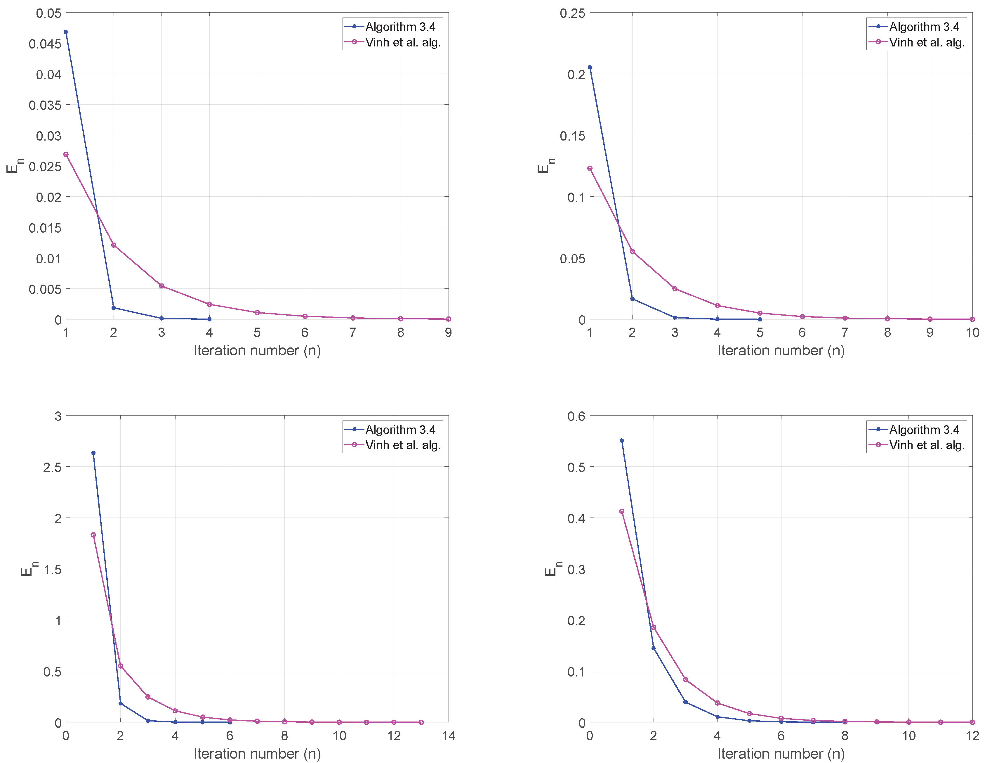
Example 2.

Let $H_1=H_2=L^2\left([0,1]\right)$ with norm $\left|\right|x\left|\right|={\left({\int }_0^1{\left|x\left(t\right)\right|}^{2}dt\right)}^{12}$ and the inner product $\langle x,y\rangle ={\int }_0^{1}x\left(t\right)y\left(t\right)dt.$ We defined the nonempty, closed convex sets $C=\{x\in L^2\left([0,1]\right):\langle x\left(t\right),3t^2\rangle =0\}$ and $Q=\{y\in L^2\left([0,1]\right):\langle y,t3\rangle \ge -1\}$. We defined the linear operator $A:L^2\left([0,1]\right)\to L^2\left([0,1]\right)$ by $\left(Ax\right)\left(t\right)=x\left(t\right).$ The projection onto C and Q are given by

$$P_C\left(x\left(t\right)\right)=\left\{\begin{array}{cc}x\left(t\right)-\frac{\langle x\left(t\right),3t^2\rangle }{\parallel 3t^2{\parallel }^2}3t^2\hfill & \mathit{if}\langle x\left(t\right),3t^2\rangle \ne 0,\hfill \\ x\left(t\right),\hfill & \mathit{if}\langle x\left(t\right),3t^2\rangle =0,\hfill \end{array}\right.$$

and

$$P_Q\left(y\left(t\right)\right)=\left\{\begin{array}{cc}y\left(t\right)-\frac{\langle y\left(t\right),\frac{-t}{3}\rangle }{\parallel -\frac{t}{3}{\parallel }^2}\left(\frac{-t}{3}\right),\hfill & \mathit{if}\langle y\left(t\right),\frac{-t}{3}\rangle <-1,\hfill \\ y\left(t\right)\hfill & \mathit{if}\langle y\left(t\right),\frac{-t}{3}\rangle \ge -1.\hfill \end{array}\right.$$

We consider the MSSFP where $k=t=1$, $C_i=C,$$Q_j=Q,$$S_m=I$ (identity mapping) and $m=4$. We compare our Algorithm 2 with the CQ-type algorithm (Algorithm 3.1) of Vinh et al. [20]. For Algorithm 2, we take $g_n\left(x\right)=\frac{x}{8},$$\beta =0.5$, $w_i=1,$${\alpha }_n=\frac{1}{n+1},$${ϵ}_n=\frac{1}{{(n+1)}^2},$ and ${\gamma }_{n,m}=\frac{1}{5}$ for $m=0,1,\dots ,4.$ Also, for Vinh et al. alg, we take ${\rho }_n=\frac{n}{n+1}$ and ${\beta }_n=\frac{1}{n+1}.$ We use $E_n=\frac{1}{2}\left|\right|A{x}_n-P_Q\left(A{x}_n\right){\parallel }^2<{10}^{-4}$ as stopping criterion and test the algorithms for the following initial points:

Case I: $x_0=exp(-2t),$$x_1=t^{3}sin\left(3t\right)3,$

Case II: $x_0=t^2+2t-1,$$x_1=(cos\left(2t\right)+sin\left(3t\right))5,$

Case III: $x_0=2tcos(-3t),$$x_1=4sin\left(2t\right),$

Case IV: $x_0=exp\left(2t\right)2,$$x_1=t^3+3t-1.$

The numerical results are reported in

Table 2. Computation result for Example 2.

		Algorithm 2	Vinh et al. alg.
Case I	No of Iter.	4	9
	CPU time (s)	0.4563	1.3020
Case II	No of Iter.	5	10
	CPU time (s)	1.5565	3.1576
Case III	No of Iter.	9	13
	CPU time (s)	0.8736	2.4094
Case IV	No of Iter.	8	12
	CPU time (s)	0.7985	1.1278

and Figure 2.

5. Conclusions

In this paper, we introduce a generalized viscosity approximation method with self-adaptive stepsize for finding common solution of multiple set split feasibility problem and fixed point of a countable family of k-strictly pseduononspreading mappings in real Hilbert spaces. We also introduce a generalized viscosity approximation method with inertial and self-adaptive stepsize for solving the underlying problem. We prove strong convergence results for the sequences generated the algorithms under some mild conditions. We also provide some numerical example to show the performance of the proposed methods with respect to some other methods in the literature. These results improve and compliment several other results (e.g., [6,7,8,9,20]) in the literature.