Modeling the Dispersion of E. coli in Waterbodies Due to Urban Sources: A Spatial Approach
by
 , , and
Kyna Borel
1,* ,
,
Vaishali Swaminathan
1,
Cherish Vance
1,
Galen Roberts
2,
Raghavan Srinivasan
3 and
and
Raghupathy Karthikeyan
1 1
Biological and Agricultural Engineering Department, Texas A&M University, 2117 TAMU, College Station, TX 77843, USA
2
North Texas Municipal Water District, 505 E Brown St, Wylie, TX 75098, USA
3
Spatial Science Laboratory in the Department of Ecosystem Science and Management, Texas A&M University, College Station, TX 77845, USA
*
Author to whom correspondence should be addressed.
Water 2017, 9(9), 665; https://doi.org/10.3390/w9090665
Submission received: 7 August 2017
/
Revised: 17 August 2017
/
Accepted: 29 August 2017
/
Published: 2 September 2017
Abstract
:In the United States, pathogens are the leading cause for rivers and streams to exceed water quality standards. The Spatially Explicit Load Enrichment Calculation Tool (SELECT) was developed to estimate bacterially contaminated water bodies based on spatial factors such as land use, soil, and population density. SELECT was originally automated using Visual Basics for Applications (VBA), which is no longer supported by the current version of ArcGIS. The aim of this research was to develop a new SELECT interface, pySELECT, using the Python programming language and to incorporate a rainfall-runoff E. coli transport module to simulate E. coli loads resulting from urban sources, such as dogs and on-site wastewater treatment systems. The pySELECT tool was applied to Lavon Lake, a semi urban study watershed in Northeast Texas. The highest potential E. coli loads were in the areas closest to the Dallas-Fort Worth metroplex, and the highest transported loads were located downstream from those identified hotspots or where the most runoff was generated. Watershed managers can use pySELECT to develop best management practices on the specific areas and fecal sources that contribute fecal contamination into a waterbody.
1. Introduction
In the United States, 54% of assessed rivers and streams are considered impaired, exceeding regulatory standards for contaminants. Among these impaired rivers and streams, pathogens are the leading cause of impairment [1]. To address bacterial impairment, several models and tools have been developed to assess contaminated water bodies, such as the Spatially Explicit Load Enrichment Calculation Tool (SELECT). Complex mechanistic models such as Hydrologic Simulation Program Fortran (HSPF) and Soil Water Assessment Tool (SWAT) simulate the fate and transport of bacteria. However, these models require large amounts of input data, which is difficult in areas with limited monitoring records [2,3,4,5]. In lieu of complex mechanistic models, SELECT was developed as an estimation tool to inform watershed management decisions
SELECT was developed to characterize E. coli sources based on spatial factors such as land use, source population density, and soil [6]. SELECT has been used to assess potential hotspots and sources of bacterial contamination in watersheds as part of watershed protection plan and total maximum daily load projects [6,7,8,9,10,11,12,13]. SELECT was originally automated within Geographic Information Systems (GIS) using Visual Basics for Applications (VBA). Users could parameterize specific water bodies using a Graphical User Interface (GUI) [7].
However, VBA is not supported by the current version of ArcGIS. Also, the VBA coded version of SELECT, hereafter referred to as SELECT VBA, uses data that are not publicly available or difficult to obtain for many watersheds. SELECT VBA does not account for bacterial transport into waterbodies. When estimating E. coli loads, pollutant connectivity to the waterbody should be included. Fate and transport of non-point source fecal microbes is driven by hydrology [4]. Therefore, an ideal microbial model should include land use, climate, topography, and hydrology [14,15]. To account for the transport of E. coli and estimate concentrations, a rainfall-runoff model utilizing the curve number method was applied within SELECT [8]. This methodology can be applied to identify potential hotspots and determine whether they contribute to the bacteria load in the waterbody [8].
Failing on-site wastewater treatment systems (OWTS) and dog feces deposited on the land surface pose a risk to human health by potentially contaminating surface waters. Approximately 23% of all homes in the United States use OWTS to treat their household sewage, typically individual buildings or small clusters of buildings that serve fewer than 20 people [16]. OWTS typically consist of a septic tank and a soil absorption field [16]. Most material settles in the septic tank, and then the remaining effluent is partially treated through the anaerobic digestion of organic matter. Once discharged to the soil absorption field, the effluent is further treated through various biological processes in the soil [16]. The United States Environmental Protection Agency (USEPA) estimates that 10% to 20% of OWTS are failing due to age, hydraulic overloading, or problems with design, installation, and maintenance [16]. In Texas, approximately 1.5 million (13%) OWTS are considered to be chronically malfunctioning which is consistent with what is happening nationally [17]. Dogs are considered a major non-point source of fecal pollution in urban and suburban areas [18]. Failing OWTS and dogs are significant domestic sources contributing to fecal contamination in waterbodies.
The objective of this research was to (1) implement a modeling scheme that applied the SELECT methodology for use in the current version of ArcGIS using Python; (2) develop a GUI for domestic fecal sources using publically accessible data; and (3) apply an E. coli transport model using the curve number method. To estimate potential and transported E. coli loads, Map Algebra and Spatial Analyst functions were incorporated into a new tool: pySELECT.
2. Materials and Methods
PySELECT is written in Python and uses the ArcPy package to access the geoprocessing functions in ArcGIS. Python (www.python.org) is an open-source, interpreted, objected-oriented programming language that has simple and easy to read syntax [19,20]. Because Python is open-source, there are thousands of Python packages that the user can use to perform specialized functions including linking code written in a different programming language into Python [20]. PySELECT is integrated into ArcGIS (10.3 and 10.4) using an ArcToolset with the modules attached as individual scripts. Four modules are included in pySELECT: Rainfall runoff (USDA-NRCS curve number), E. coli transport, and potential E. coli load (dogs and OWTS).
2.1. Spatial Data Layers
The previous VBA version of SELECT required input data layers that were difficult to obtain for areas lacking a governmental GIS department. Therefore, pySELECT was developed using free and publicly available information (Table 1).
2.2. Graphical User Interface
The pySELECT GUI contains four individual forms connected to the Python script modules (Figure 1). These forms allow the user to select and customize the input data layers. The GUI interacts with ArcGIS by showing the available layers from the map document. The output raster files are input into the map document as part of the python script. Output from the E. coli load modules (dogs and OWTS) provide inputs to the E. coli transport module. The interface was developed with these modules as a standalone script.
2.3. Potential E. coli Load Module: Dogs
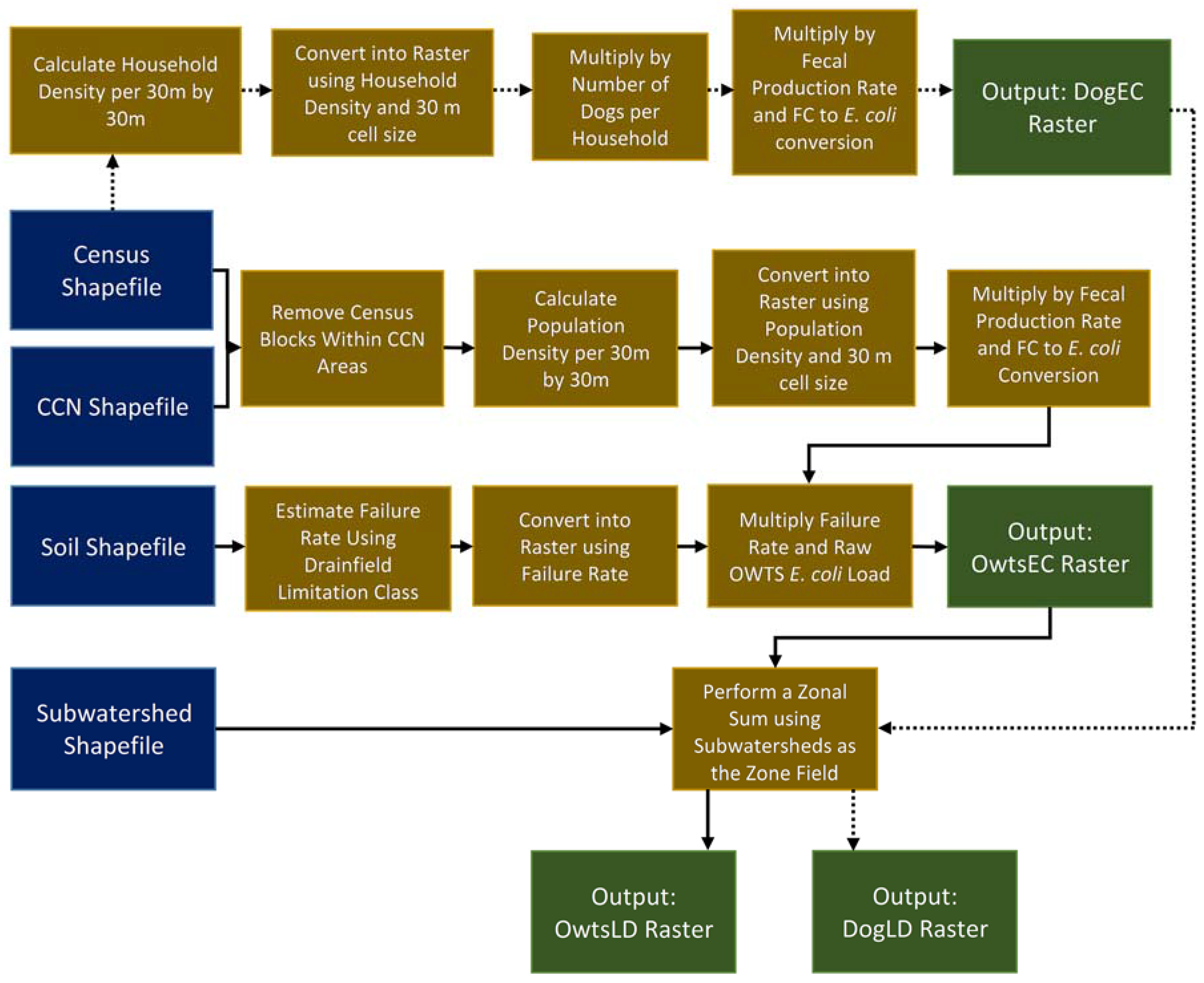
The number of dogs in the watershed are estimated using the number of households and the number of dogs per household. The household density within each census block was calculated per 900 m2 to match the raster cell size during conversion. The dog population density is estimated by multiplying the household density by the number of dogs per household (Figure 2). Potential E. coli load from dogs is calculated by multiplying the dog population density by the dog fecal production rate and the fecal coliform to E. coli conversion factor (Figure 2). The potential E. coli load resulting from dogs per grid cell is then converted into a raster file (DogEC) and inserted into the map document (Figure 2). Default values for the dog fecal production rate (5 × 10⁹ fecal coliforms/dog/day) and the fecal coliform to E. coli conversion factor (0.63) can be adjusted by the user [27]. The conversion factor was based on the historical USEPA regulatory standards for fecal coliform and E. coli in recreational waters: 200 CFU/100 mL and 126 CFU/100 mL, respectively [28].
To compare with the original SELECT VBA results, the potential E. coli load sum per subwatershed was calculated. The DogEC raster is used as the value raster input when performing a zonal sum using the subwatershed shapefile as the zone field. The resulting raster provides the potential E. coli load resulting from dogs per subwatershed which is more useful for visually comparing areas that contribute bacterial contamination. The potential E. coli load sum per subwatershed (DogLD) is added to the map document (Figure 2).
2.4. Potential E. coli Load Module: OWTS
To estimate the potential E. coli load resulting from OWTS, the areas without OWTS were removed from the census blocks. The certificate of convenience and necessity (CCN) is a shapefile containing polygons for areas that are serviced by wastewater treatment plants [24]. The census blocks within areas serviced by sewer, determined by the CCN, were deselected so that the remaining census blocks presumably used OWTS (Figure 2). The population density within each census block was calculated per 900 m2 to match the raster cell size during conversion. The population density raster was then multiplied by the raw sewage fecal production rate and the fecal coliform to E. coli conversion factor to estimate the E. coli load per grid cell of raw sewage per day (Figure 2). The default value for the raw sewage fecal production rate (2.65 × 10¹⁰ fecal coliforms/person/day) can be modified by the user. The default fecal production rate was calculated by multiplying the fecal coliform concentration (up to 105 fecal coliforms/mL per USEPA) in raw sewage [27] by the volume of wastewater produced per person per day (265 L/person/day) [7].
A failure rate was then applied to the E. coli load of raw sewage because every OWTS in the watershed is not failing simultaneously. The failure rate was estimated using the drainfield limitation class field in the soils shapefile. The drainfield limitation class indicates the suitability for use in septic tank absorption fields based on the soil’s properties. The soils are rated based on the hazard or risk associated with a particular use: “not limited” poses little to no risk and “very limited” has high risk [29]. The failure rate was classified for not rated, very limited, somewhat limited, and not limited classes as 8, 15, 10, and 5%, respectively. The soils shapefile was then converted to a raster (30 m × 30 m) using the failure rate as the value field. The potential E. coli load for OWTS per grid cell (OwtsEC) was calculated by multiplying the failure rate by the E. coli load of raw sewage.
Similar to the potential E. coli load module for dogs, the potential E. coli load per subwatershed (OwtsLD) is calculated using the OwtsEC raster and the subwatershed shapefile.
2.5. Rainfall-Runoff and E. coli Transport
The curve number module uses the USDA-NRCS curve number look-up table [30] and assumes antecedent moisture condition (AMC) II. The USDA-NRCS curve number look-up table is hardcoded into the curve number module, therefore the input land use data layer must be NLCD land use or a shapefile that uses the same classification scheme. The soil input layer must have the hydrologic soil groups labeled as A, B, C, and D. The land use and soils shapefiles are overlaid to create polygons with unique land use and soil hydrologic soil groups (Figure 3). The curve number is calculated for each unique polygon and then converted to raster (30 m × 30 m).
Runoff is estimated using the soil conservation service (SCS) curve number method [30,31]. The maximum soil water retention parameter is calculated as:
where S is the maximum soil water retention parameter (mm) and CN is the curve number. The runoff volume was calculated as:
where Q is the runoff volume (mm × m2), P is the precipitation (mm), S is the maximum soil water retention parameter (mm), and A is the area of the grid cell (m2).
The runoff volume is estimated per grid cell using map algebra. Precipitation is input by the user and uniformly applied to the watershed. If the watershed is large (with rain gauge data for multiple stations), the rain gauges average could be used. Otherwise, the watershed area could be delineated first, and then pySELECT applied to separate subwatersheds. After runoff volume is calculated as a raster, it is used as the weight raster to calculate runoff accumulation. The flow accumulation tool requires an input of flow direction and an optional weight raster input. The accumulated flow is the accumulated weight of all cells flowing into each downslope of the output raster [32]. The flow direction input raster is created from a digital elevation model (DEM), bare earth elevation map, using the DEM fill tool followed by the flow direction tool [26]. The resulting accumulation output raster (AccRunoff) provides runoff volumes for each grid cell. The AccRunoff output raster is added to the map document once it was created (Figure 3).
The accumulated E. coli output raster is estimated by first calculating the runoff volume per grid cell. The runoff volumes per grid cell are then converted into a binary runoff grid (0 or 1). If any runoff occurs on that cell, it is assigned a value of 1. Otherwise, runoff does not occur and it is assigned a value of zero.
The OwtsEC or DogEC raster calculated using the potential E. coli load module for dogs or OWTS is used as the input E. coli load raster. The E. coli load is multiplied by the binary runoff grid to create the weight raster. This ensures that the areas contributing to the accumulated E. coli load also have runoff. The accumulated E. coli output raster (AccEcoli) is calculated using the flow accumulation tool with the weight raster and the flow direction raster as inputs.
To aid in output visualization, subwatershed zonal maximums are calculated for the AccRunoff and AccEcoli rasters: RunZoneMax and ecolisubmax, respectively. The RunZoneMax raster shows the maximum runoff accumulation within each subwatershed. The ecolisubmax raster shows the maximum transported E. coli load located within the subwatershed. These visualizations illustrate the potential E. coli hotspots caused by runoff transport of E. coli attributable to domestic sources, such as dogs or OWTS.
3. Tool Verification
3.1. Study Watershed
Lavon Lake is a drinking water source reservoir located on the East Fork of the Trinity River. The watershed that drains into Lavon Lake encompasses 198,911 ha (491,520 ac) and is located in the North Texas counties of Collin, Grayson, Fannin, and Hunt (Figure 4). Most of the watershed is undeveloped or agricultural land (87%) (Figure 5); however, North Texas is one of the fastest growing areas in the nation currently consisting of 13% developed land [33]. Two contributing tributaries, Wilson Creek and the East Fork of the Trinity River, were identified as impaired due to bacteria [34]. To address this impairment, SELECT was used to estimate E. coli loads for the development of the Lavon Lake Watershed Protection Plan (WPP).
3.2. E. coli Transport Model Workflow
All spatial files were first projected to NAD 1983 UTM Zone 14N. This projection was chosen to maintain consistency of units (meters) for the area calculations. Before specifying inputs in the module forms, the workspace folder location should be designated for the creation of intermediate and output files. The user then selects spatial inputs from the drop down menu or by searching the file manager. Default values are not provided for the dog per household input in the potential E. coli load module for dogs or the precipitation amount input in the E. coli transport module. The U.S. average is 0.6 dogs per household [35]. However, local veternarians and stakeholders suggested the watershed population was higher than the U.S. average; therefore, 1.25 dogs per household was used for the Lavon Lake watershed. The default fecal production rate and fecal coliform to E. coli conversions were used [12]. The raw sewage fecal production rate of 3.08 × 10¹² fecal coliforms/person/day was used. The runoff accumulation and E. coli accumulation for the Lavon Lake watershed were estimated using a 2-year, 24-h storm event: Appoximately 101.6 mm (4 in) [36].
3.3. Results
The accuracy of the potential E. coli load resulting from dogs and potential E. coli load resulting from OWTS modules were verified by comparing the output results with the manually calculated results for the dog and OWTS potential E. coli loads for the Lavon Lake watershed To manually calculate the results, the individual processes were performed in ArcGIS using the same input files.
The RunZoneMax output raster showed the areas where the most runoff was generated from the 2-year, 24-h storm event. The subwatersheds to the east of Lavon Lake had the highest amount of runoff generated (Figure 6).
The DogEC and OwtsEC output rasters showed the locations with the highest potential E. coli load. However, this output is not very useful for watershed managers. Therefore, the DogLD and OwtsLD rasters are used when communicating results to watershed managers and stakeholders.
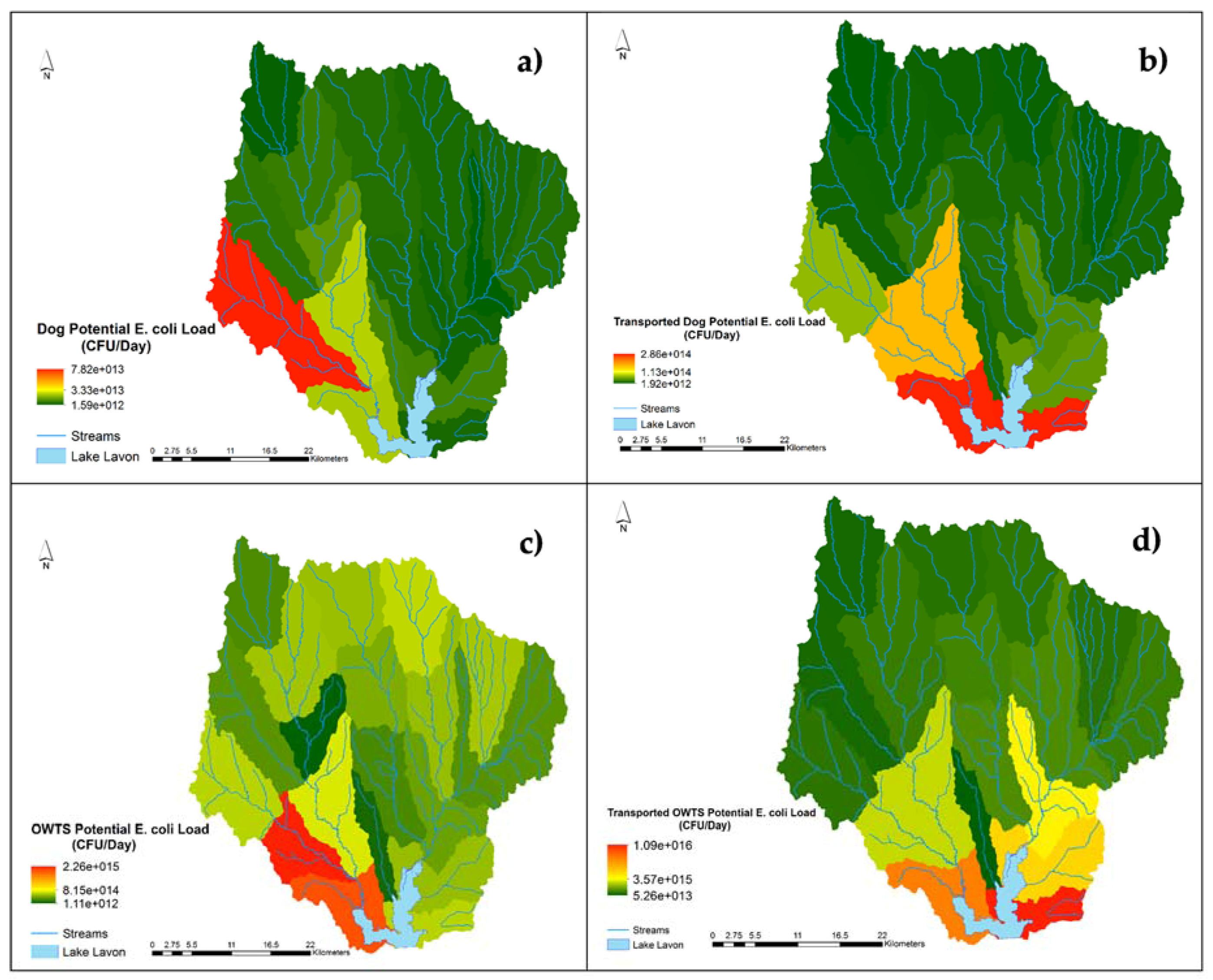
Dogs contributed the highest potential E. coli load in the western most subwatersheds, which are closest to the Dallas-Fort Worth metroplex (Figure 7a). The E. coli accumulation mirrored the untransported potential E. coli load result with the highest transported E. coli loads contributed by dogs occurring in the same area to the west of Lavon Lake (Figure 7b). Therefore, the subwatersheds contributing the highest transported potential E. coli loads (resulting from dogs) were located downstream from the previously identified hotspots in Figure 7a.
The areas with the highest potential E. coli load due to failing OWTS were located in the subwatersheds to the west of Lavon Lake (Figure 7c). The most runoff accumulation occurred to the east of Lavon Lake. However, the largest potential E. coli contributions from failing OWTS came from the subwatersheds located west of Lavon Lake in the areas closest to the Dallas-Fort Worth metroplex. The E. coli accumulation reflects a combination of both source location and transport from runoff. After potential E. coli loads due to OWTS were transported, the two areas that contributed most to bacterial contamination were immediately to the west and east of Lavon Lake (Figure 7d).
4. Discussion
4.1. Applications of pySELECT
The pySELECT tool shows contamination hotspots based on source location and watershed hydrology, which can enable watershed managers to more effectively apply best management practices for watershed remediation. The previous version of SELECT did not show whether potential E. coli loads would be transported into a waterbody; therefore, it was possible that potential hotspot areas did not contribute microbial contamination.
Because pySELECT uses publicly available input data, it can be applied in areas without specific data on OWTS and household locations, such as most rural areas. Additionally, pySELECT has customizable inputs, which enables the user to make the model more representative of their study area. The tool can be applied to any watershed in the United States where a CCN GIS layer is available.
4.2. Limitations
The tool currently includes several hardcoded parameters: NLCD land use values, hydrologic soil groups, and curve numbers. These hard-coded parameters decrease the versatility of the script, limiting inputs to those only with the proper classification system. Another limitation is the amount of preprocessing required for the input layers. Shapefiles require a spatial projection with a linear unit of meters. Otherwise, the population distribution grid, which is calculated for meters, would be inaccurate. Also, the census shapefile requires specific attributes: Population field and household field, which contain the population and number of households per census block, respectively. Lastly, the soil shapefile (input for the potential E. coli load module for OWTS) requires the drainfield limitation class field in the attribute table. Future development of pySELECT will focus on increasing user flexibility by removing hard-coded values and broadening the types of allowable input.
As a simple tool, pySELECT does not simulate the complex processes typically used in watershed bacterial models. The tool was design with ease of use as a priority. Therefore, E. coli growth and die-off are not accounted for in pySELECT. In-stream bacteria concentrations are spatially and temporally variable, which contributes to the difficulty in modeling bacteria [3,5]. However, pySELECT results provide a snapshot of potential E. coli loads [9].
5. Conclusions
To include pollutant connectivity and better estimations of domestic source contributions, an updated version of SELECT, pySELECT, was programmed in Python. Updates included a graphical user interface and four modules: Potential E. coli load modules for dogs and OWTS, a rainfall runoff (USDA-NRCS curve number) module, and an E. coli transport module. The pySELECT results from the potential E. coli load modules for dogs and OWTS were verified with manual calculations for the Lavon Lake watershed case study. The curve number and E. coli transport modules simulate the transport of potential E. coli loads from dog and OWTS sources. Versatile and easy to use, pySELECT can be applied to almost any area of interest in the United States with publicly available input data layers. Watershed managers can use pySELECT to focus best management practices on the specific areas and fecal sources that contribute fecal contamination into a waterbody.
Acknowledgments
This work was supported by a state nonpoint source program grant from the Texas State Soil and Water Conservation Board (TSSWCB) [FY 2016 Workplan 16–62]. The sponsor (TSSWCB) had no involvement in the publication of this article. We acknowledge the thoughtful feedback of three anonymous reviewers that improved the quality of this manuscript.
Author Contributions
Kyna Borel, Vaishali Swaminathan, Raghavan Srinivasan, and Raghupathy Karthikeyan conceptualized the model. Galen Roberts provided information about the watershed. Kyna Borel wrote the paper and performed the programming. Cherish Vance, Galen Roberts, and Raghupathy Karthikeyan edited the manuscript for technical content.
Conflicts of Interest
The authors declare no conflict of interest.
References
- National Summary of State Information. Available online: https://ofmpub.epa.gov/waters10/attains_nation_cy.control (accessed on 31 August 2017).
- Ferguson, C.M.; Croke, B.F.; Beatson, P.J.; Ashbolt, N.J.; Deere, D.A. Development of a process-based model to predict pathogen budgets for the Sydney drinking water catchment. J. Water Health 2007, 5, 187–208. [Google Scholar] [PubMed]
- Frey, S.K.; Topp, E.; Edge, T.; Fall, C.; Gannon, V.; Jokinen, C.; Marti, R.; Neumann, N.; Ruecker, N.; Wilkes, G. Using SWAT, Bacteroidales microbial source tracking markers, and fecal indicator bacteria to predict waterborne pathogen occurrence in an agricultural watershed. Water Res. 2013, 47, 6326–6337. [Google Scholar] [CrossRef] [PubMed]
- Pachepsky, Y.A.; Sadeghi, A.M.; Bradford, S.A.; Shelton, D.R.; Guber, A.K.; Dao, T. Transport and fate of manure-borne pathogens: Modeling perspective. Agric. Water Manag. 2006, 86, 81–92. [Google Scholar] [CrossRef]
- Saleh, A.; Du, B. Evaluation of SWAT and HSPF within BASINS program for the upper North Bosque River watershed in central Texas. Trans. ASAE 2004, 47, 1039–1049. [Google Scholar]
- Teague, A.; Karthikeyan, R.; Babbar-Sebens, M.; Srinivasan, R.; Persyn, R.A. Spatially explicit load enrichment calculation tool to identify potential E. coli sources in watersheds. Trans. ASABE 2009, 52, 1109–1120. [Google Scholar] [CrossRef]
- Riebschleager, K.J.; Karthikeyan, R.; Srinivasan, R.; McKee, K. Estimating Potential Sources in a Watershed Using Spatially Explicit Modeling Techniques. J. Am. Water Res. Assoc. 2012, 48, 745–761. [Google Scholar] [CrossRef]
- Borel, K.E.; Karthikeyan, R.; Smith, P.K.; Srinivasan, R. Predicting E. coli concentrations in surface waters using GIS. J. Nat. Environ. Sci. 2012, 3, 19–33. [Google Scholar]
- Borel, K.E.; Karthikeyan, R.; Smith, P.K.; Gregory, L.F.; Srinivasan, R. Estimating daily potential E. coli loads in rural Texas watersheds using Spatially Explicit Load Enrichment Calculation Tool (SELECT). Tex. Water J. 2012, 3, 42–58. [Google Scholar]
- Borel, K.; Karthikeyan, R.; Berthold, T.A.; Wagner, K. Estimating E. coli and Enterococcus loads in a coastal Texas watershed. Tex. Water J. 2015, 6, 33–44. [Google Scholar]
- Roberts, G.; McFarland, M.; Lloyd, J.; Helton, T.J. Mill Creek Watershed Protection Plan. 2015. Available online: http://millcreek.tamu.edu/files/2014/09/MillCreekWPP.pdf (accessed on 1 September 2017).
- NTMWD; Texas A&M Agrilife Extension Service; TSSWCB Lavon Lake Watershed Protection Plan. 2017. Available online: https://www.ntmwd.com/wp-content/uploads/2017/05/Lavon-Lake-WPP_DRAFT_June2017.pdf (accessed on 1 September 2017).
- Glenn, S.M.; Bare, R.; Neish, B.S. Modeling bacterial load scenarios in a Texas coastal watershed to support decision-making for improving water quality. Tex. Water J. 2017, 8, 57–66. [Google Scholar]
- Coffey, R.; Cummins, E.; Bhreathnach, N.; Flaherty, V.O.; Cormican, M. Development of a pathogen transport model for Irish catchments using SWAT. Agric. Water Manag. 2010, 97, 101–111. [Google Scholar] [CrossRef]
- Jamieson, R.; Gordon, R.; Joy, D.; Lee, H. Assessing microbial pollution of rural surface waters: A review of current watershed scale modeling approaches. Agric. Water Manag. 2004, 70, 1–17. [Google Scholar] [CrossRef]
- Otis, R.; Kreissl, J.F.; Frederick, R.; Goo, R.; Casey, P.; Tonning, B. Onsite Wastewater Treatment Systems Manual (EPA/625/R-00/008); U.S Environmental Protection Agency: Washington, DC, USA, 2002.
- Study to determine the magnitude of, and reasons for, chronically malfunctioning on-site sewage facility systems in Texas. 2001. Available online: https://www.tceq.texas.gov/assets/public/compliance/compliance_support/regulatory/ossf/StudyToDetermine.pdf (accessed on 1 September 2017).
- Mallin, M.A.; Williams, K.E.; Esham, E.C.; Lowe, R.P. Effect of human development on bacteriological water quality in coastal watersheds. Ecol. Appl. 2000, 10, 1047–1056. [Google Scholar] [CrossRef]
- Lin, J.W. Why Python is the next wave in earth sciences computing. Bull. Am. Meteorol. Soc. 2012, 93, 1823–1824. [Google Scholar] [CrossRef]
- Sanner, M.F. Python: A programming language for software integration and development. J. Mol. Graph. Model. 1999, 17, 57–61. [Google Scholar] [PubMed]
- Homer, C.G.; Dewitz, J.A.; Yang, L.; Jin, S.; Danielson, P.; Xian, G.; Coulston, J.; Herold, N.D.; Wickham, J.D.; Megown, K. Completion of the 2011 National Land Cover Database for the conterminous United States-Representing a decade of land cover change information. Photogramm. Eng. Remote Sens. 2015, 81, 345–354. [Google Scholar]
- Soil Data Access. Available online: https://sdmdataaccess.sc.egov.usda.gov (accessed on 31 August 2017).
- TIGER/Line® Shapefiles and TIGER/Line® Files. Available online: https://www.census.gov/geo/maps-data/data/tiger-line.html (accessed on 1 September 2017).
- CCN Mapping Information. Available online: https://www.puc.texas.gov/industry/water/utilities/gis.aspx (accessed on 31 August 2017).
- Geospatial Data Gateway. Available online: http://datagateway.nrcs.usda.gov (accessed on 31 August 2017).
- National Elevation Dataset (NED) 2013. Available online: https://tnris.org/data-catalog/entry/national-elevation-dataset-ned-2013/ (accessed on 31 August 2017).
- Edition, F.; USEPA. Protocol for Developing Pathogen TMDLs; U.S. Environmental Protection Agency: Washington, DC, USA, 2001; p. 132. Available online: https://nepis.epa.gov/Exe/ZyNET.exe/20004QSZ.txt?ZyActionD=ZyDocument&Client=EPA&Index=2000%20Thru%202005&Docs=&Query=&Time=&EndTime=&SearchMethod=1&TocRestrict=n&Toc=&TocEntry=&QField=&QFieldYear=&QFieldMonth=&QFieldDay=&UseQField=&IntQFieldOp=0&ExtQFieldOp=0&XmlQuery=&File=D%3A\ZYFILES\INDEX%20DATA\00THRU05\TXT\00000001\20004QSZ.txt&User=ANONYMOUS&Password=anonymous&SortMethod=h|-&MaximumDocuments=1&FuzzyDegree=0&ImageQuality=r85g16/r85g16/x150y150g16/i500&Display=hpfr&DefSeekPage=x&SearchBack=ZyActionL&Back=ZyActionS&BackDesc=Results%20page&MaximumPages=1&ZyEntry=2 (accessed on 1 September 2017).
- USEPA Recreational water quality criteria. 2012. Available online: https://www.epa.gov/sites/production/files/2015-10/documents/rwqc2012.pdf (accessed on 1 September).
- Soil Survey Manual; Ditzler, C.; Scheffe, K.; Monger, H.C. (Eds.) USDA Handbook 18; Government Printing Office: Washington, DC, USA, 2017.
- USDA-NRCS Urban Hydrology for Small Watersheds. 1986. Available online: ftp://ftp.odot.state.or.us/techserv/Geo-Environmental/Hydraulics/Hydraulics%20Manual/Chapter_07/Chapter_07_appendix_G/Urban_Hydrology_for_Small_Watersheds.pdf (accessed online 1 September 2017).
- Haan, C.T.; Barfield, B.J.; Hayes, J.C. Design Hydrology and Sedimentology for Small Catchments, 3rd ed.; Academic Press: San Diego, CA, USA, 1994. [Google Scholar]
- How Flow Accumulation Works. Available online: https://pro.arcgis.com/en/pro-app/tool-reference/spatial-analyst/how-flow-accumulation-works.htm (accessed on 31 August 2017).
- Lake Lavon Watershed Protection Plan Fact Sheet. Available online: https://www.ntmwd.com/documents/lavon-lake-watershed-protection-plan-fact-sheet (accessed on 31 August 2017).
- TCEQ 2014 Texas Integrated Report; Texas Commission on Environmental Quality: Austin, TX, USA, 2015.
- American Veterinary Medical Association. U.S. pet ownership & demographics sourcebook, 2012 ed.; American Veterinary Medical Association: Schaumburg, IL, USA, 2012; p. 186. [Google Scholar]
- Hershfield, D.M. Rainfall Frequency Atlas of the United States for Durations from 30 Minutes to 24 Hours and Return Periods from 1 to 100 Years; U.S. Department of Commerce: Washington, DC, USA, 1961.
Figure 1.
Example of pySELECT graphical user interface (GUI) for the OWTS module.
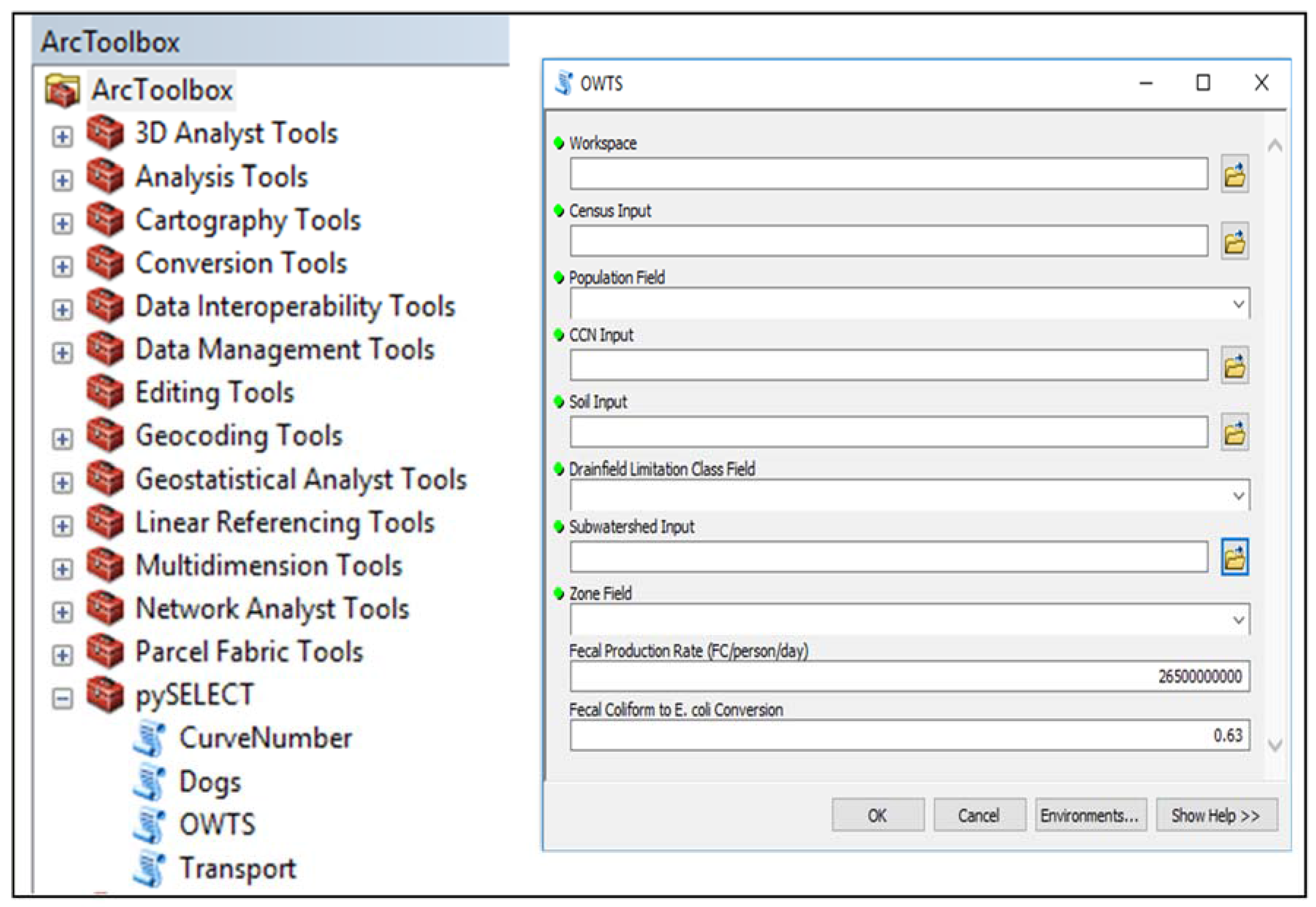
Figure 2.
Calculation of potential E. coli loads, resulting from dogs (dashed line) and OWTS (solid line), in pySELECT.
Figure 2.
Calculation of potential E. coli loads, resulting from dogs (dashed line) and OWTS (solid line), in pySELECT.

Figure 3.
Rainfall-Runoff Module (blue) and E. coli Transport Module (green) processes in pySELECT.
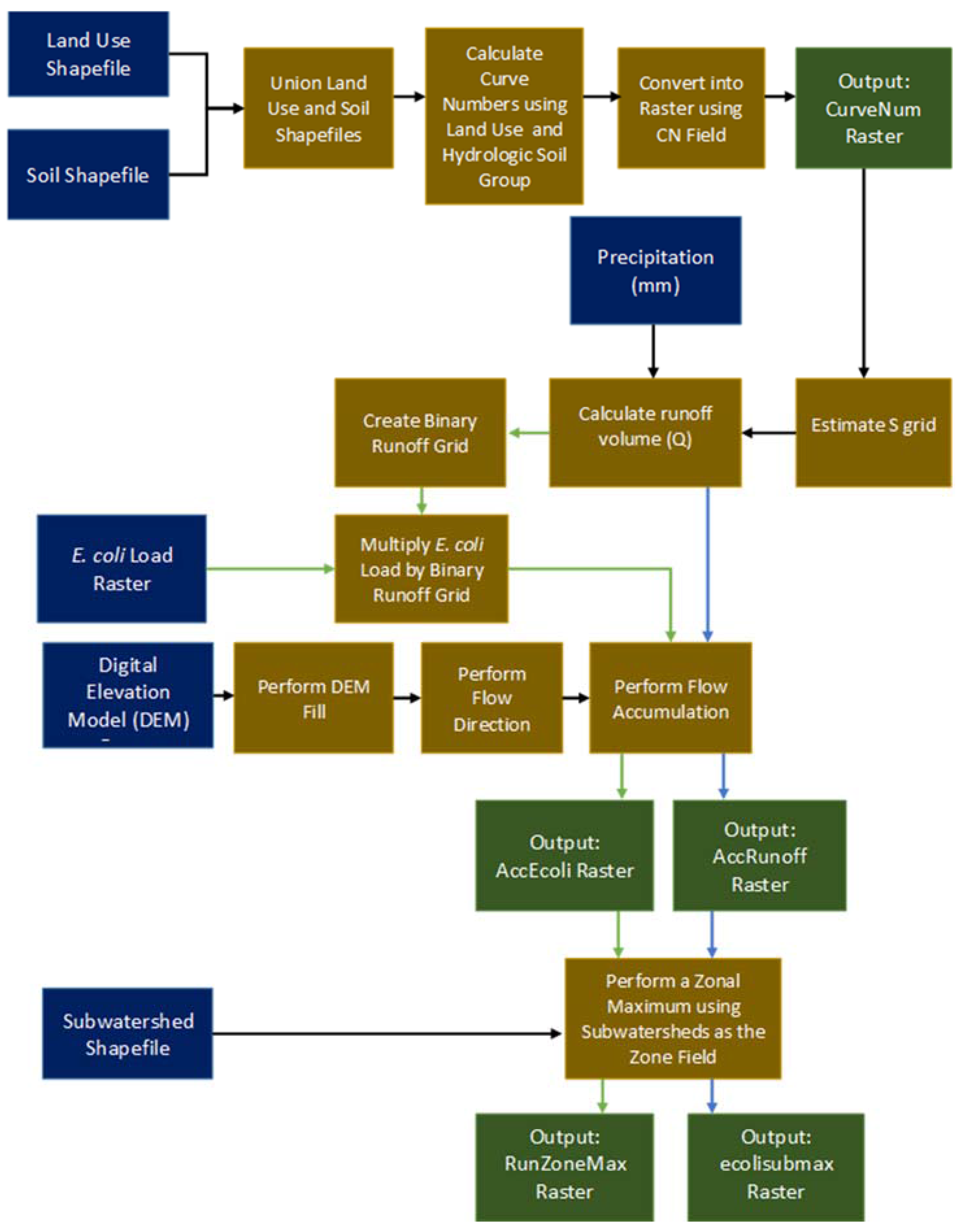
Figure 4.
Location of Lavon Lake watershed with delineated subwatersheds and stream network.
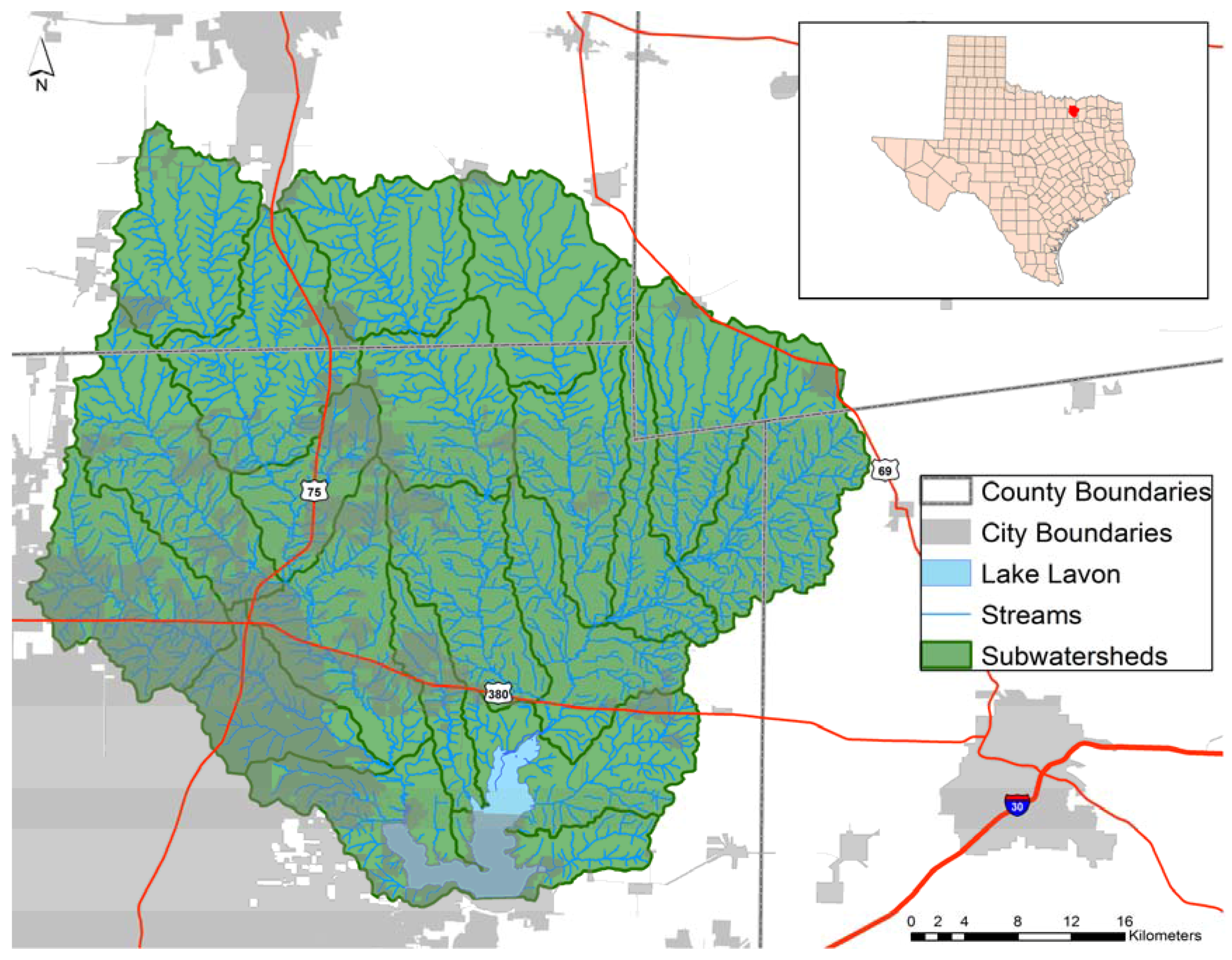
Figure 5.
Land use land cover of the Lavon Lake watershed.
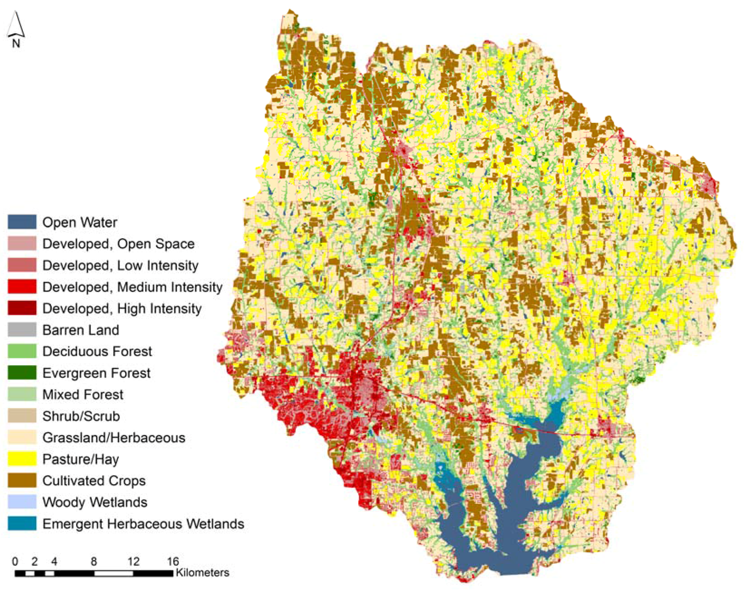
Figure 6.
Accumulated runoff subwatershed maximum due to a 2-year, 24-h storm event in the Lavon Lake watershed.
Figure 6.
Accumulated runoff subwatershed maximum due to a 2-year, 24-h storm event in the Lavon Lake watershed.
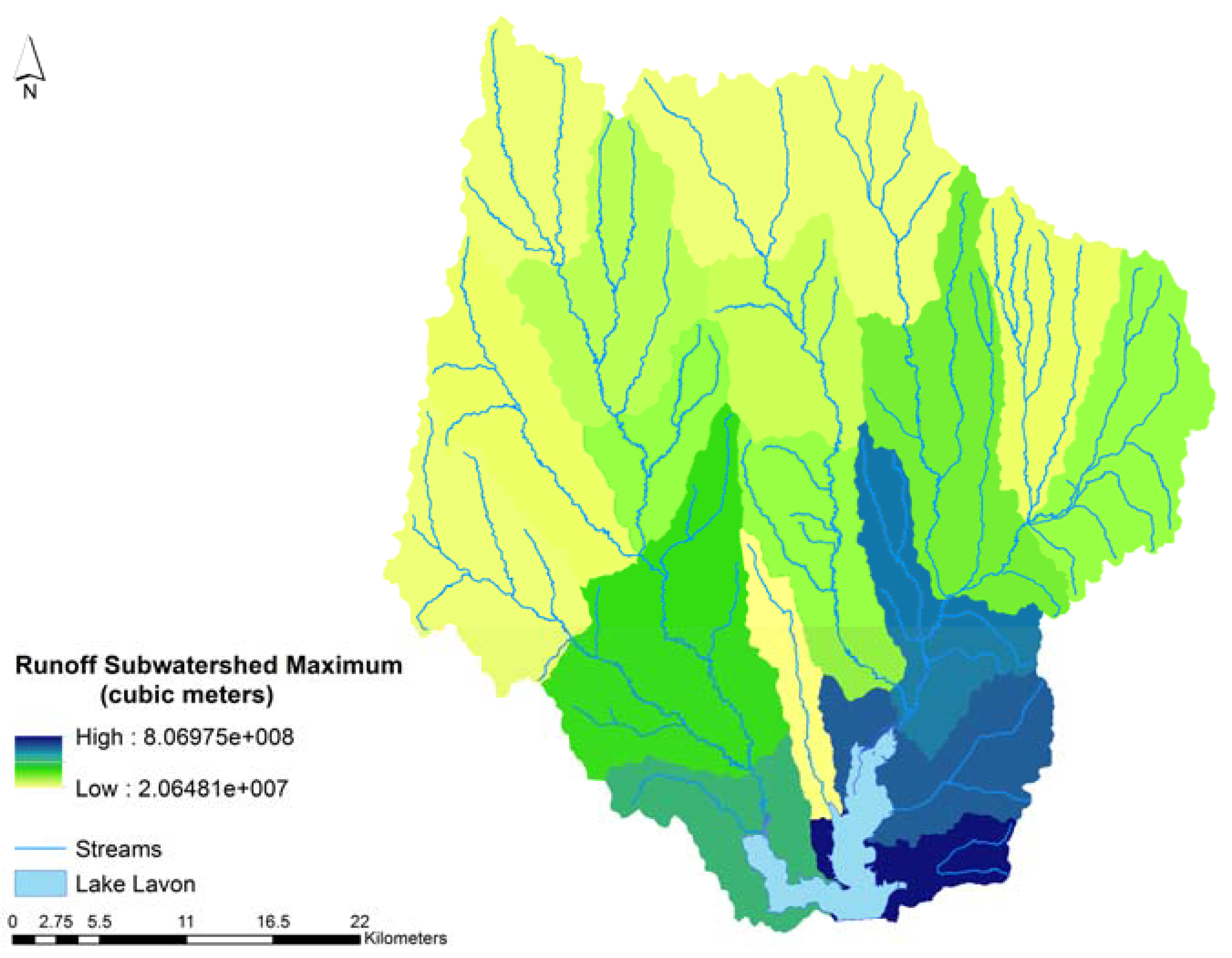
Figure 7.
Potential E. coli load subwatershed summation from (a) dogs and (c) OWTS in the Lavon Lake watershed. Subwatershed maximum transported potential E. coli load from (b) dogs and (d) OWTS due to a 2-year, 24-h storm event in the Lavon Lake watershed.
Figure 7.
Potential E. coli load subwatershed summation from (a) dogs and (c) OWTS in the Lavon Lake watershed. Subwatershed maximum transported potential E. coli load from (b) dogs and (d) OWTS due to a 2-year, 24-h storm event in the Lavon Lake watershed.

© 2017 by the authors. Licensee MDPI, Basel, Switzerland. This article is an open access article distributed under the terms and conditions of the Creative Commons Attribution (CC BY) license (http://creativecommons.org/licenses/by/4.0/).
Share and Cite
MDPI and ACS Style
Borel, K.; Swaminathan, V.; Vance, C.; Roberts, G.; Srinivasan, R.; Karthikeyan, R. Modeling the Dispersion of E. coli in Waterbodies Due to Urban Sources: A Spatial Approach. Water 2017, 9, 665. https://doi.org/10.3390/w9090665
AMA Style
Borel K, Swaminathan V, Vance C, Roberts G, Srinivasan R, Karthikeyan R. Modeling the Dispersion of E. coli in Waterbodies Due to Urban Sources: A Spatial Approach. Water. 2017; 9(9):665. https://doi.org/10.3390/w9090665
Chicago/Turabian StyleBorel, Kyna, Vaishali Swaminathan, Cherish Vance, Galen Roberts, Raghavan Srinivasan, and Raghupathy Karthikeyan. 2017. "Modeling the Dispersion of E. coli in Waterbodies Due to Urban Sources: A Spatial Approach" Water 9, no. 9: 665. https://doi.org/10.3390/w9090665
Note that from the first issue of 2016, this journal uses article numbers instead of page numbers. See further details here.