Urban Runoff Characteristics in Combined Sewer Overflows (CSOs): Analysis of Storm Events in Southeastern Spain

Abstract

Storm water overflows have an important impact on the environment in many European countries. Nowadays, a better knowledge of combined sewer overflows (CSOs) pollution is required for implementing measures to reduce these emissions. In this work, pollution flows mobilized during rainy events have been monitored and modeled in two urban catchments located in the city of Murcia (southeast Spain). For each analyzed event, rainfall volume, in-sewer turbidity and water flow depth have been continuously measured. Therefore, sets of pollutographs and hydrographs have been obtained for each event analyzed. Characteristic variables have been defined and obtained for each event such as the maximum concentration of turbidity, the total event rainfall, the previous dry weather period, the time to the peak of the hydrograph and to the peak of the pollutograph, among others. Relations between variables have been adjusted through a statistical model. The adjusted parameters are used to generate pollutographs that are compared with those measured in field. The present work provides tools to assist in the knowledge of pollution transported through sewer network during stormy events, suggesting the creation of design pollutographs which may facilitate the evaluation of measures to reduce urban runoff pollution.

1. Introduction

The reduction of pollution emissions from combined sewer overflows (CSOs) is currently a prime issue. Actually, European Directives aim to quantify and reduce them to protect the environment and human health, and to provide water leisure activities and water abstraction for agriculture [1]. Although a lack of knowledge of the quantity and the quality of these overflows is recognized and policies have yet to be achieved in most countries, important efforts are being done (e.g., [2,3,4,5]). Risk based approaches are usually implemented taking into account the type of collecting systems and the intensity of the rain events or flooding. Spill frequency, or volume percentage retained, are habitually selected [4,6]. Other approach is the receiving water quality criteria, based on Urban Pollution Management procedures (UPM) standards [5]. It requires being aware of ecological state of receiving water and effects induced by the pollution. Field measurement campaigns of the urban sub-catchment are recommended as a previous step to implement an approach [3,7,8] so that pollution mobilized during rain events can be evaluated.

Continuous water-quality monitoring sensors are being increasingly implemented in sewers. In order to replace traditional sampling, turbidimeters can be used to estimate total suspended solids (TSS) and chemical oxygen demand (COD) concentration in sewers, by linear regression of on-site turbidity with site-specific measurements [7,8,9,10,11,12,13].

The relationship between pollutant load of TSS and runoff, by statistical approaches, constitutes a field of research to identify pollution associated to CSOs [7,14,15,16,17,18,19,20]. In this way, measured hydrographs and pollutographs analysis are used to relate the peak of the pollutant concentration of the flow, and the mass and flow cumulative volume curves M(V), which, for instance, allow determining whether the first flush effect exists for a particular catchment [7,14,15,16,17]. Suarez and Puertas [17] fitted the maximum suspended solids concentration (C_MAXSS) by means of probability distributions. With regard to rainy events, several researchers [7,18,19,20] performed regression analysis between TSS and hydrological and hydraulic variables (Table 1). These statistical models gave rise to adjusted pollution parameters, which can be used for forecasting transported pollution characteristics along storm events, providing useful information to establish effective policies of combined sewer overflow control. As these studies are usually catchment specific, an important aim would be to define standard coefficients for a wide range of catchment conditions [18].

Table 1. Variables and adjusted parameters of TSS pollution load.

Variables and Adjusted Parameters			Gupta and Saul [18]	LeBoutillier et al. [19]	Gromaire et al. [20]	Del Rio [7]
Variables	Hydrology	Imax (mm/h)	X	X	X
		Drain (h)	X	X		X
		DWP (day)	X	X	X
		RD (mm)		X	X	X
		Imax5 (mm/h)		X
		Tc (h)				X
		A (ha)				X
	Hydraulic	Qmax (m3/s)	X			X
		Qmean (m3/s)				X
		Qmaxdw (m3/s)				X
		TPH (h)				X
		TPP (h)				X
Adjusted parameters		TSSTE (kg/event)		X
		TSSff (kg/event)	X		X
		CMAXSS (mg/L)				X
		CSMSS (kg/ha)				X

Notes: I_max = maximum rainfall intensity; D_rain = rainfall duration; DWP = dry weather period; RD = rain depth; I_max5 = maximum five-minute rainfall intensity; T_c = time of concentration of the catchment; A = catchment area; Q_max = maximum event inflow; Q_mean = mean event inflow; Q_maxdw = maximum dry weather inflow; TPH = time to the peak of the hydrograph; TPP = time to the peak of the pollutograph; TSS_TE = cumulative suspended solids per event; TSS_ff = total pollutant load in the first flush; C_MAXSS = maximum suspended solids concentration; and C_SMSS = specific mobilized volume of suspended solids.

For a proper design of sustainable sewer systems, hydraulic and quality modeling tools are utilized [8,19,21]. Hydraulic models, such as USEPA Storm Water Management Model (SWMM) [22], predict the runoff flow rate and volume from observed rainfall intensities with accuracy. However, for quality models, the uncertainty is an order of magnitude greater than that for the hydraulic submodels [23]. That makes their calibration and use complex.

In this work, statistical models are proposed to predict the event maximum turbidity concentration (C_MAXtb), the time to the peak of the pollutograph (TPP), and the time to the descent of pollutograph (TDP).

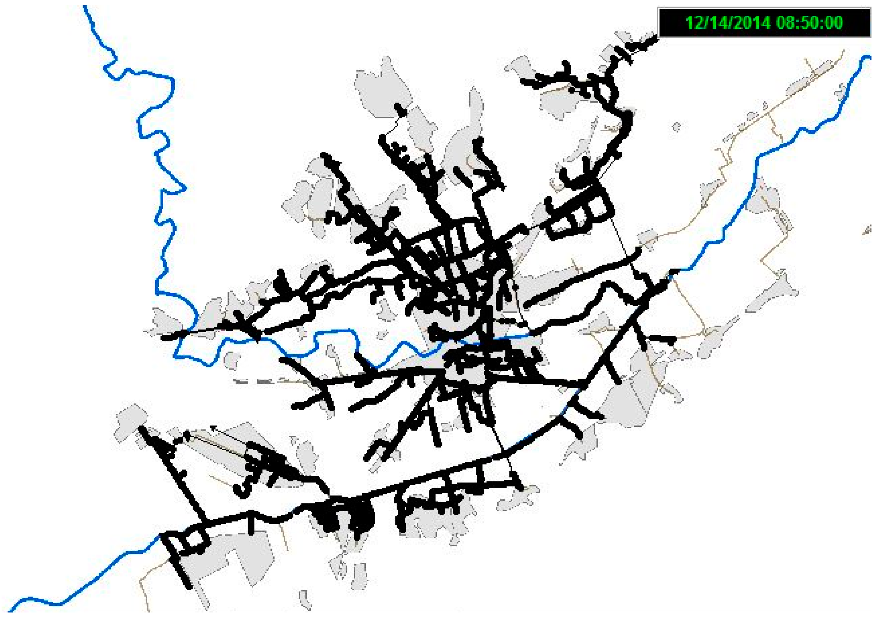
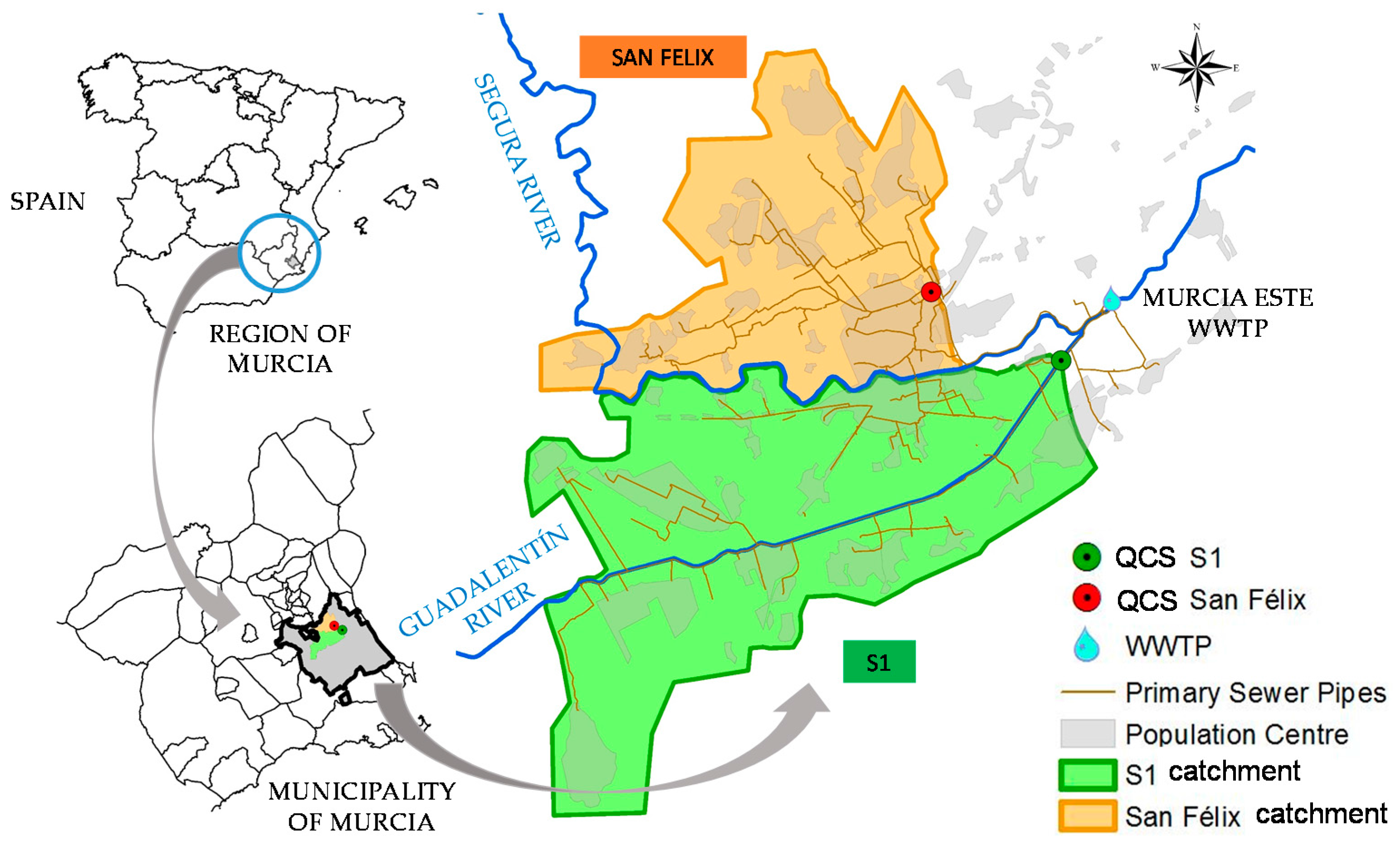
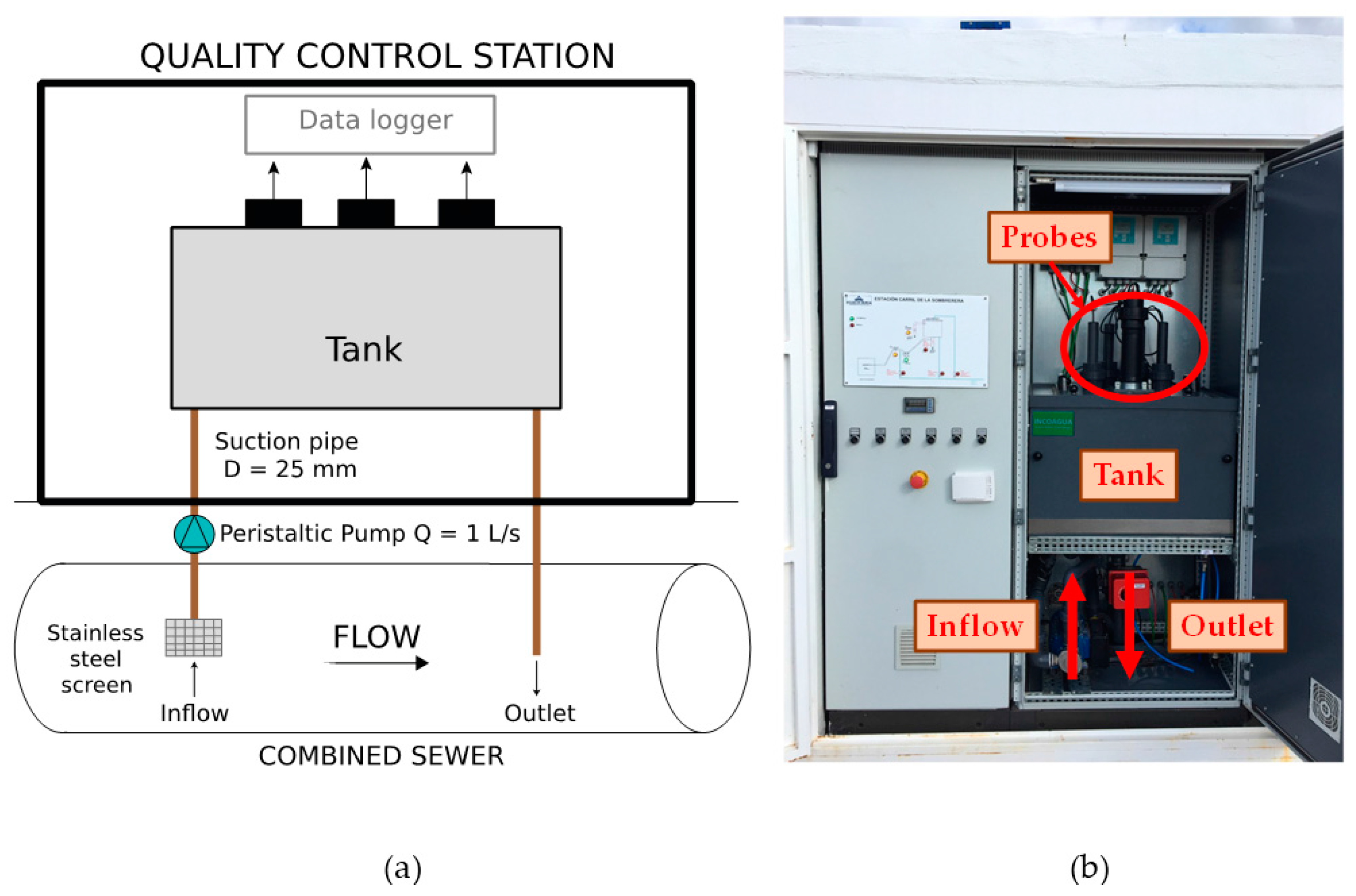
The statistical models are based upon analysis of data collected from rainfall events during period from June 2014 to April 2016 at two urban catchments in the city of Murcia (southeast Spain). Both catchments were monitored with continuous measurements from rain gauges, in-sewer turbidimeters and water gauges. Several input parameters of the statistical models were considered to assess their significance, and the most significant parameters were selected. Predicted pollutograph parameters are calculated and modeled. The proposed pollutographs are compared with the measured ones showing a significant agreement. A calibrated hydraulic model of the city of Murcia has been generated in the USEPA Storm Water Management Model (SWMM). The numerical model is used to analyze the catchment hydraulic response to each rainfall event.

The present work provides tools to assist in the knowledge of pollution transported through sewer network during stormy events, suggesting the creation of design pollutographs which may facilitate the evaluation of measures to reduce urban runoff pollution.

2. Experimental Methods

2.1. Description of the Experimental Catchment Areas

Murcia is a southeastern Spanish city with an equivalent population of 525,027. It is situated in a valley at the confluence of the Guadalentín and Segura rivers (Figure 1). The study site includes two urban catchments, called San Félix and S1. Both catchments are residential areas, their impervious areas being 21% and 47%, respectively (Table 2). The sewer system is combined incorporating storm water. Due to the flat topographic conditions, there are several sewer pump stations. Both catchments flow into “Murcia Este” Wastewater Treatment Plant whose maximum capacity during dry weather is Q_maxdw = 10.000 m³/h. At the outlet pipe of each catchment, monitoring equipments were placed in Quality Control Stations (QCS) (Figure 1).

Figure 1. Location of the study site.

Table 2. Catchments description.

Catchment	San Félix	S1
Area of catchment (km2), A	14.89	47.53
Population density (inh/km2)	14,250	2685
Ratio of imperviousness (m2/m2)	0.47	0.21
Mean slope (m/m), S	0.0043	0.0013
Catchment flow length (km), L	10.75	17.00
Length combined sewerage (km)	513.15	616.84

The catchment slope was estimated from a Digital Elevation Model with a 2 m × 2 m grid, using ArcGIS 10.3 software. The catchment flow length was obtained from the sewer network geodatabase of the Empresa Municipal de Aguas y Saneamiento de Murcia S.A. (Emuasa).

2.2. Monitoring Equipment

The city of Murcia is equipped with 39 tipping-bucket rain gauges that cover the different catchments. Their measurements range is between 0 and 7 mm/min, with an accuracy of 0.2 mm. Data are continuously sent and plotted through a SCADA system.

Monitoring equipments were placed at the outlet sewer pipe of the analysed catchments, close to an important overflow point (Figure 1). They consisted of a water gauge to continuously monitor the flow. The water level was measured with an ultrasonic sensor Endress + Hauser FMR50. The wastewater circulating in sewers is continuously pumped by means of a 1 L/s peristaltic pump to a 20 L sedimentation tank, through a suction 25 mm-diameter pipe inserted in the sewer and protected by a screen of stainless steel to trap sediments (Figure 2). Wastewater passes through a 20 L tank, in which the probes are located. The probes measure turbidity, conductivity and temperature. Data are recorded within a 20 s time interval. The turbidity data are obtained with an infra-red nephelometric turbidimeter Endress + Hauser CUS 42 measuring at a wavelength of 880 nm according to the standard NF EN 27027, associated to a data logger. A backwash proccess with clear water is automatized each hour to avoid disturbing measurements. Turbidimeters are calibrated with formazine solution. A technique for the removal of these outliers has been implemented.

Figure 2. (a) Scheme of Quality Control Station devices; and (b) Image of QCS.

The rating curve for each monitoring station was developed in previous studies. There is a control section-free overfall in the Quality Control Station of San Felix. A water level measurement is used in the Quality Control Station of S1. Velocity sensors were used in a straight conduit of 1.8 m diameter and around 1000 m length, where uniform conditions were confirmed.

2.3. Hydraulic Model

The US Environmental Protection Agency’s Storm Water Management Model (USEPA) is a numerical model that allows simulating the hydrological and hydraulic behavior of an urban drainage system. A calibrated SWMM hydraulic model of the city of Murcia has been used. It serves to study the catchment response to any rainfall event (Figure 3). The characteristics of the model are shown in Table 3. The total length of the network included in the model is around 234.5 km.

Figure 3. View of the hydraulic model of Murcia in USEPA Storm Water Management Model (SWMM).

Table 3. Description of the hydraulic model of Murcia.

Description	Element	Number
Hydrology	Pluviographs	39
	Subcatchments	4553
Hydraulics	Nodes	6073
	Outfalls	58
	Tanks	70
	Links	6304
	Pump stations	100

The Horton equation was used for infiltration modeling. Values adopted are in accordance with soil characteristics and with those proposed in the literature [21,22]. The maximum infiltration, f₀, is around 20 mm/h, while the minimum infiltration, f_c, is 1 mm/h. The decay coefficient, k, has been estimated at 4.14 h⁻¹. The Manning’s roughness coefficients for pervious and impervious areas were used as calibration parameters of the model. Initial values were selected from the literature [21,22]: 0.02–0.045 for pervious areas and 0.01–0.015 for impervious areas. The Manning roughness coefficient for conduits varies from 0.011 to 0.013 depending on the pipe material.

The comparison of the measured and simulated flow depth is shown in Figure 4. In wet weather, two different events are presented. Some differences are found in S1 Catchment, whereas a quite good agreement is observed in San Felix Catchment. Those differences, which are below 10%, are caused by pump stations.

Figure 4. Flow depth measured and calculated by the hydraulic model during wet weather at Quality Control Stations S1 and San Felix.

From the hydraulic model, the time of concentration, T_c, is obtained for each catchment. The concentration time, T_c, may be decomposed into two terms: overland runoff time, T_E, and in-sewer run time, T_R [3]:

$$T_c=T_E+T_R$$

(1)

A common expression to calculate T_c in non-urban catchments is presented by Temez [24]:

$$T_{c\_rural}=0.3\frac{L^{0.76}}{S^{0.19}}$$

(2)

where L is the longest overland flow length (km), and S the mean catchment slope (-).

Values calculated from the hydraulic model and presented in Table 4 adjust to the Temez equation modified for urban areas [25]:

$$T_c=\frac{T_{c\_rural}}{1+3\sqrt{\mu \left(2-\mu \right)}}$$

(3)

where T_c is the concentration time modified for urban catchments that takes into account the in-sewer run time, and μ is the fraction of the area that is impervious. The time of concentration of the catchment was obtained introducing a uniform precipitation in each sub-catchment with a duration higher enough to assure that all the surface contributes to the outfall.

Table 4. Comparison of the modified concentration time.

Catchment	Concentration Time, Tc (min)
	Hydraulic Model	Equation (3)
S1	193.75	200
San Felix	87.14	80

The values of the modified concentration time, T_c, calculated by the hydraulic model and by Equation (3) are presented in the following table:

3. Results and Discussion

3.1. Variables Definition from Wet Weather Measured Events

The data registered from monitoring rainfall events corresponds to the period from June 2014 to April 2016 at both urban catchments. During this period, 10 storm events were measured in the S1 QCS and 9 in the San Felix QCS.

Measured values are presented in Table 5 and Table 6 for San Felix and S1, respectively. All rainfalls exceed the total amount of 2 mm, which is the minimum value to assure runoff.

Table 5. Variables of rainfall events at San Felix Catchment.

San Felix Catchment
Event code	SF_1	SF_2	SF_3	SF_4	SF_5	SF_6	SF_7	SF_8	SF_9
Year	2014	2014	2015	2015	2015	2015	2015	2016	2016
Date (dd-m)	17 June	14 December	22 March	11 June	5 September	27 September	15 January	9 May	4 June
PTOTAL (mm)	7.34	30.71	2.47	10.13	56.47	7.53	11.57	6.80	2.27
Imean (mm/h)	4.63	1.23	0.99	1.40	2.26	2.44	2.28	1.01	2.27
Imax10 (mm/h)	19.67	8.86	2.76	5.32	18.76	5.28	4.71	4.84	6.04
DWP (days)	15	10	1	22	19	17	17	18	22
Qmax (L/s)	2710	2930	1580	2530	3170	2590	2650	2260	1680
Qmean (L/s)	945.00	1396.53	746.67	1217.95	1726.96	1073.25	1173.92	989.42	680.19
Qmax/Qmeandw	10.04	10.85	5.85	9.37	11.74	9.59	9.81	8.37	6.22
TPH (min)	35	60	105	80	95	130	205	180	90
EV (m3)	32,493	155,853	25,536	64,308	195,837	38,637	60,222	46,305	22,038
EVdw (m3)	10,467	31,638	11,028	17,046	30,993	9846	15,729	13,149	10,335
EVww (m3)	22,026	12,4215	14,508	47,262	164,844	28,791	44,493	33,156	11,703
Eww/EVdw	0.68	0.80	0.57	0.73	0.84	0.75	0.74	0.72	0.53
CMAXtb (NTU)	626	851	481	770	994	765	830	498	593
EMCtb (NTU)	251	279	286	319	270	308	440	301	318
TPP (min)	64.81	99.88	111.89	110.18	132.82	128.67	165.61	156.51	64.81

Table 6. Variables of rainfall events at S1 Catchment.

	S1 Catchment
Event code	S1_1	S1_2	S1_3	S1_4	S1_5	S1_6	S1_7	S1_8	S1_9	S1_10
Year	2014	2014	2014	2015	2015	2015	2015	2016	2016	2016
Date (dd-m)	24 June	22 September	14 December	20 May	11 June	27 September	15 January	30 January	21 March	4 April
PTOTAL (mm)	12.06	3.29	30.37	3.03	8.69	8.18	11.16	14.19	27.48	13.46
Imean (mm/h)	1.90	0.67	1.22	1.35	1.16	2.80	2.09	3.70	0.99	0.71
Imax10 (mm/h)	4.24	2.55	7.62	3.86	4.24	5.87	5.33	8.25	4.39	7.05
DWP (days)	7	5	10	24	22	17	17	15	13	12
Qmax (L/s)	2360	1520	2480	1560	2350	2430	2440	1970	2150	2580
Qmean (L/s)	1567.34	960.00	1617.77	790.00	1393.44	1580.00	1690.00	1190.00	1700.87	1390.00
Qmax/Qmeandw	5.06	3.10	5.22	2.55	4.49	5.10	5.45	3.84	7.81	4.48
TPH (min)	130.0	175.2	110.0	150.0	150.0	109.8	205.2	145.2	155.0	135.0
EV (m3)	74,292	32,349	184,911	32,628	75,246	50,091	65,745	63,048	210,663	99,084
EVdw (m3)	12,975	10,242	36,918	14,592	18,495	10,884	12,891	14,661	39,162	21,297
EVww (m3)	61,317	22,107	147,993	18,036	56,751	39,207	52,854	48,387	171,501	77,787
Eww/EVdw	0.83	0.68	0.80	0.55	0.75	0.78	0.80	0.77	0.81	0.79
CMAX (mg/L)	588	522	788	822	767	652	698	728	564	496
EMCtb (NTU/L)	174	257	171	299	226	229	292	239	147	237
TPP (min)	96.03	107.12	100.37	103.06	105.33	90.19	120.65	110.65	119.82	104.76

Several variables have been calculated from the monitored data and are also collected in Table 5 and Table 6, such as the total rainfall volume P_TOTAL, the maximum rainfall intensity during ten minutes I_max10, the mean intensity I_mean, and the number of antecedent dry days DWP. There are also others parameters such as the maximum runoff flow rate Q_max, the mean runoff flow rate Q_mean, the time to hydrograph peak TPH, the total runoff volume EV, the part of the runoff volume that would correspond to dry weather EV_dw, the difference between both EV_ww, the maximum turbidity registered during the episode C_MAXtb, the mean event turbidity value EMC_tb, and the time to the peak of pollutograph TPP.

These variables have been calculated for all rainfalls, which are hereinafter used to study the correlation among them to adjust statistical models that allow predicting several variables at any rainfall event, e.g., the event maximum turbidity concentration C_MAXtb, and the time to the peak of pollutograph TPP.

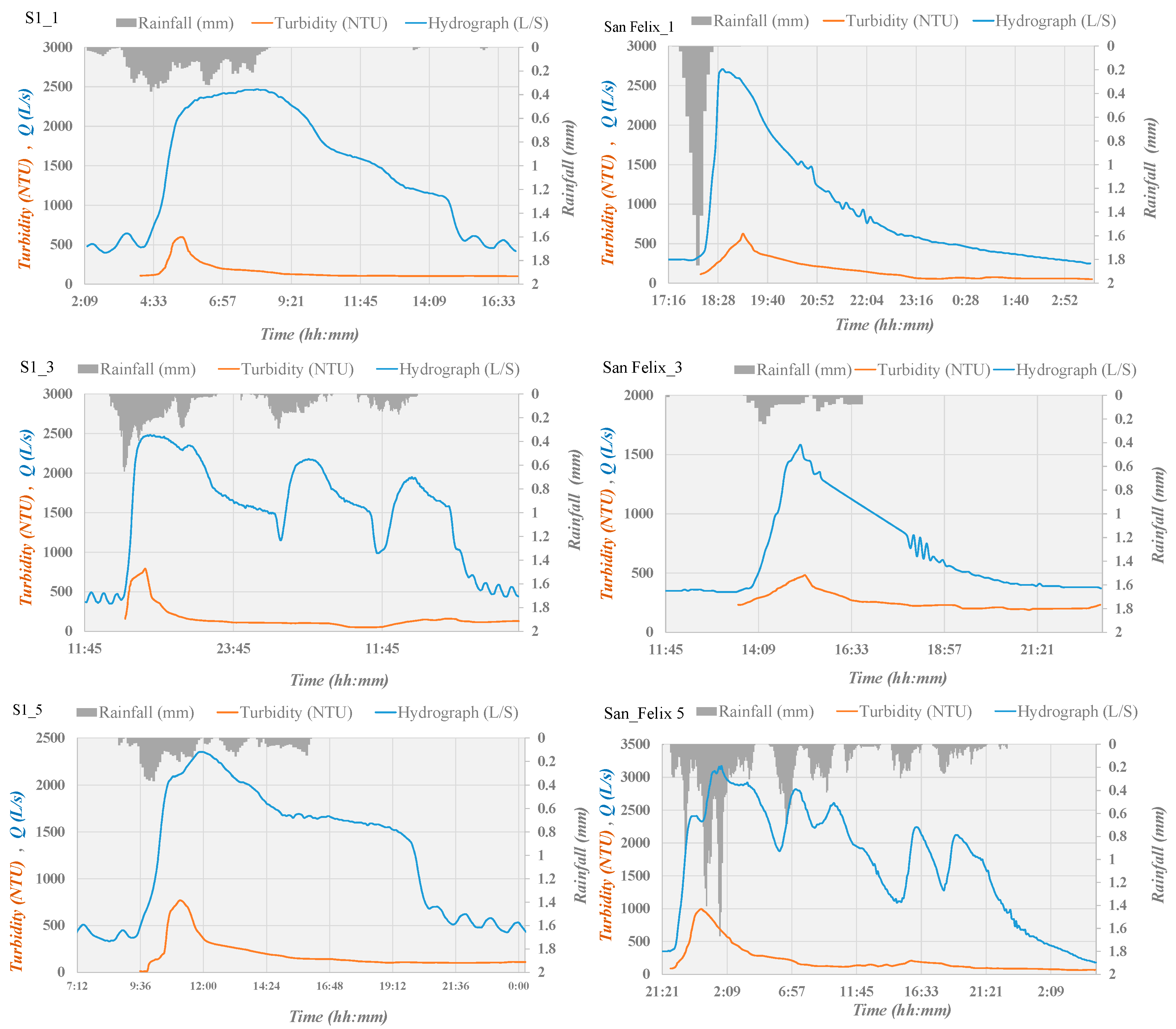
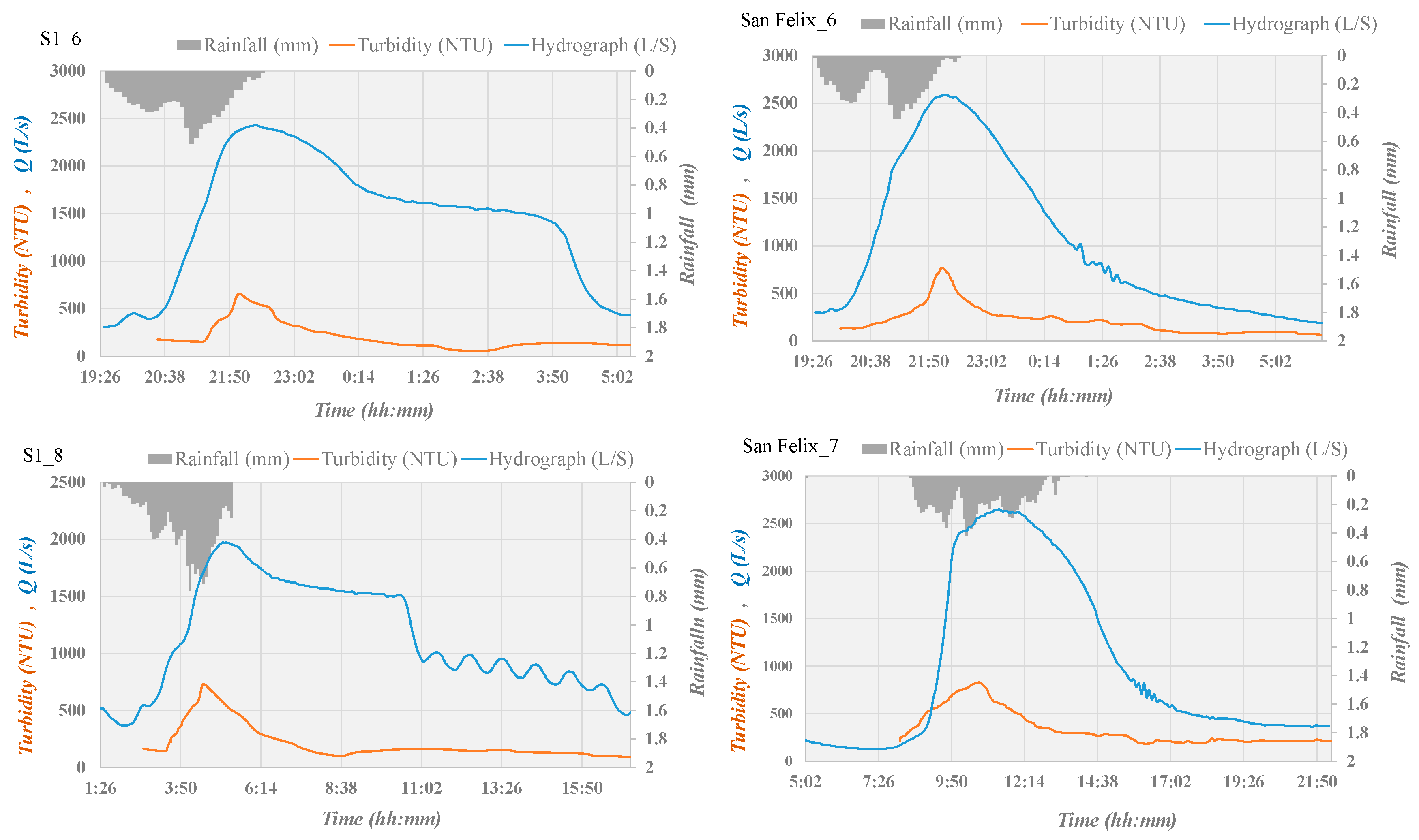
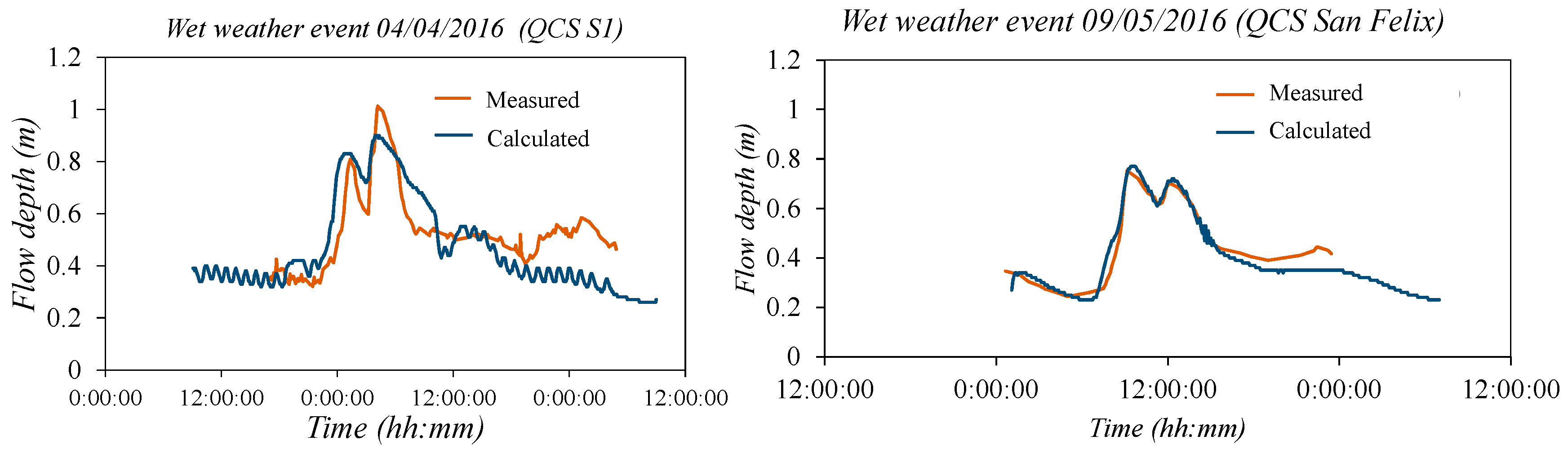
The hydrographs and turbidity-pollutographs of some of the measured rainfall events are presented in Figure 5. The pollutograph peak does not always precede the hydrograph one, as can be observed in Table 5 and Figure 5 for San Felix Catchment.

Figure 5. Rainfall, hydrographs and turbidity-pollutograph of events: S1_1; S1_3; S1_5; S1_6; S1_8; San Felix_1; San_Felix_3; San Felix_5; San Felix_6; and San Felix_7.

The calibrated hydraulic model in SWMM has been used to obtain the hydrographs presented in Figure 5.

3.2. Predictor Variables Correlations

With the objective of adjusting a statistical model, the correlation between predictor variables has been traced. The chosen predictor variables are DWP, Q_max, TPH, P_TOTAL, I_max10, C_MAXtb, and TPP. The correlation matrix is presented in Table 7 and Table 8 for S1 and San Felix catchments, respectively. The Pearson’s correlation coefficient has been applied to the sample of each pair of variables. From the matrices, correlation between the time to pollutograph peak, TPP, and the time to hydrograph peak, TPH, is observed with values of R² = 0.79 and 0.94 for S1 and San Felix, respectively. The dry period preceding the episode, DWP, and the maximum concentration of turbidity, C_MAXtb, show good relation, especially in the S1 Catchment with R² = 0.68. There is also certain relationship between the maximum concentration of turbidity, C_MAXtb, with the total precipitation and the maximum flow in the San Felix Catchment.

Table 7. Correlation matrix for variables of rainfall events at S1 Catchment.

	DWP	Qmax	TPH	PTOTAL	Imax10	CMAXtb	TPP
DWP	1.00	−0.01	0.09	−0.29	0.02	0.68	0.07
Qmax		1.00	−0.35	0.24	0.55	0.02	−0.31
TPH			1.00	−0.32	−0.43	−0.10	0.79
PTOTAL				1.00	0.50	0.01	0.24
Imax10		Symmetrical			1.00	0.21	−0.06
CMAXtb						1.00	−0.08
TPP							1.00

Table 8. Correlation matrix for variables of rainfall events at San Felix Catchment.

	DWP	Qmax	TPH	PTOTAL	Imax10	CMAXtb	TPP
DWP	1.00	0.28	0.12	0.10	0.13	0.32	0.19
Qmax		1.00	−0.12	0.74	0.61	0.84	0.06
TPH			1.00	−0.18	−0.61	−0.08	0.94
PTOTAL				1.00	0.59	0.80	0.11
Imax10		Symmetrical			1.00	0.48	−0.52
CMAXtb						1.00	0.16
TPP							1.00

3.3. Pollution Prediction Indexes. Statistical Model

From the previous section, the correlation between predictor variables individually analyzed is considered not significant enough to be used as a prediction tool of the pollution in a rainfall event. For this reason, multivariate indexes are proposed. The aim is to predict, on the one hand, the maximum concentration of turbidity during each event, C_MAXtb, and, on the other hand, the time elapsed from the beginning of the event until the maximum peak of the pollutograph, TPP. To achieve this, two indexes of prediction are adjusted: the time to peak of the pollutograph index, I_TPP, and the maximum concentration index, I_CMAX.

3.3.1. Time to the Peak of Pollutograph Index, I_TPP

The index time to the peak of the pollutograph will be used to predict the time that elapses from the beginning of the episode until the maximum value of turbidity in the event is reached, TPP. It can be defined with dimensionless factors:

$$I_{TPP}={\left(\frac{TPH}{T_C}\right)}^{0.13}{\left(\frac{P_{TOTAL}}{P_{TOTAL\_ANNUAL}}\right)}^{0.02}$$

(4)

where P_{TOTAL_ANNUAL} is the total precipitation expected in a year, adopting 350 mm for this region. In Equation (4), the time to the peak of the hydrograph, TPH, is considered. Its significant relation with TPP is shown in the correlation matrices (Table 7 and Table 8).

The first term of Equation (4), TPH/T_c, reflects the time of the catchment to respond as a function of: (i) how the rain is distributed proportionally to TPH; and (ii) the shape of the catchment inversely proportional to T_c. The second term, P_TOTAL/P_{TOTAL_ANNUAL}, magnitude of the rainfall, is also proportional to the time to the peak of the pollutograph. 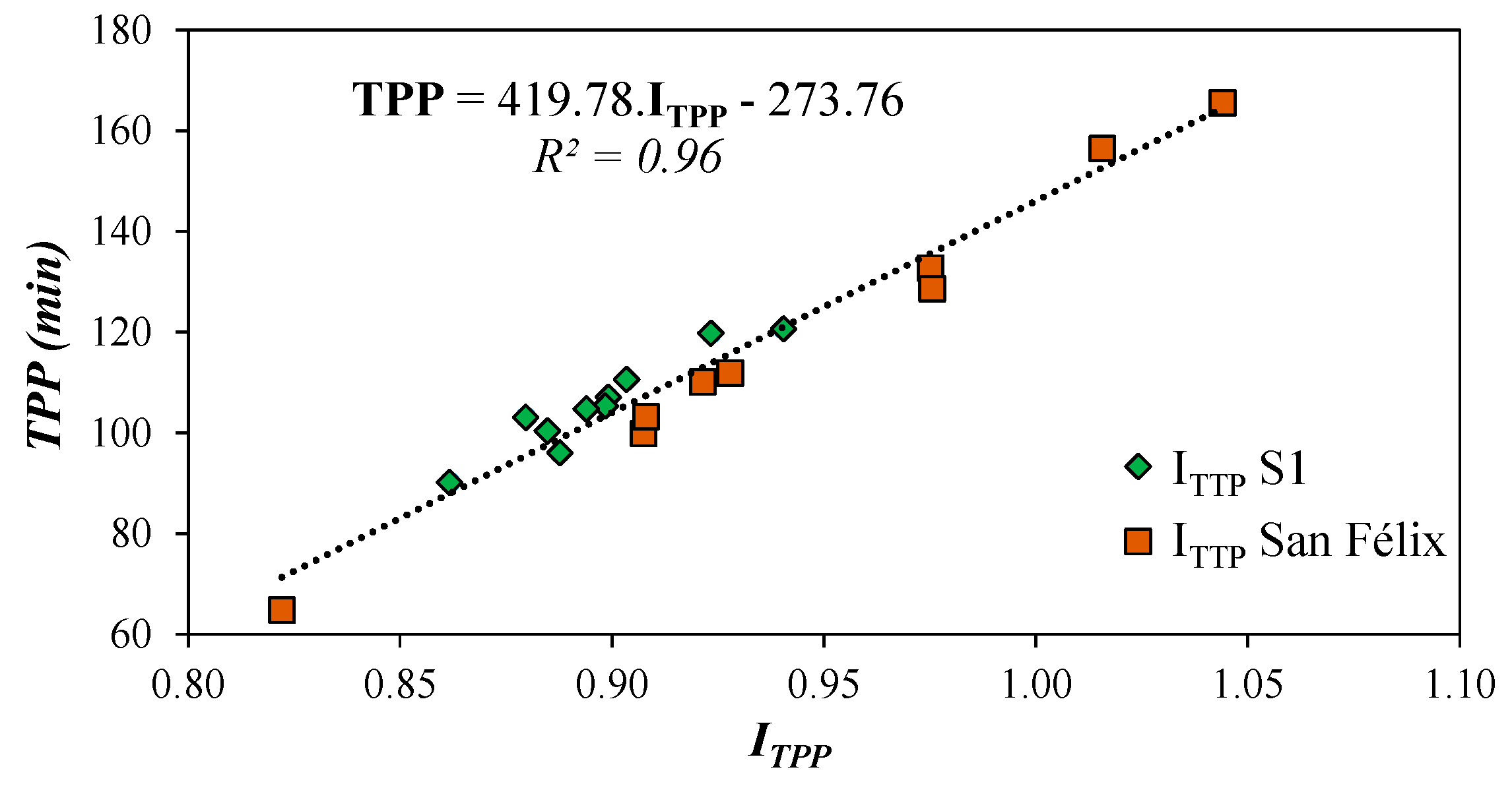In this Equation, the term P_TOTAL/P_{TOTAL_ANNUAL} has lower influence on the index than TPH/T_c. However, its inclusion improves the adjustment from R² = 0.87 to R² = 0.96. Figure 6 shows the linear relationship between the pollutograph time to the peak index, defined in previous equation, and the time to the peak of pollutograph.

Figure 6. Linear adjustment of TPP with prediction index I_TPP.

In Figure 6, a linear regression that relates the time index to the peak of the pollutograph and the time to the peak, expressed in minutes, can be obtained as:

$$TPP=419.78I_{TPP}-273.76$$

(5)

3.3.2. Maximum Concentration Index, I_CMAX

The maximum concentration index I_CMAX arises with the objective of estimating the maximum concentration of turbidity, C_MAXtb, from predictor variables quantified in rainfall events. Together with the I_TPP, they allow estimating both the magnitude of the pollutograph and the location in time of the higher turbidity. The equation for I_CMAX is defined as

$$I_{CMAX}={\left(\frac{P_{TOTAL}}{P_{TOTAL\_ANNUAL}}S\right)}^{0.3}{\left(DWR\right)}^{0.3}{F}_{shape}$$

(6)

where DWR is the proportion of consecutive dry weather days previous to the event in the last month. Equation (6) is dimensionless and can be divided into three main terms. The first term is related to the power of the event, where an increase in the total rainfall causes a greater sediment wash. Assuming the rest of parameters fixed, a higher maximum concentration will occur in the catchment with a higher average slope. The second term reflects that during the time without precipitation there is sedimentation and accumulation of deposits along the network that can be washed away during storm events. Finally, the third term is a shape factor of the catchment. It is a catchment geometric parameter defined according to

$$F_{shape}=\frac{10A}{L^2}$$

(7)

where A is the area of the catchment (km²) and L is the catchment flow length (km).

Table 9 summarizes the shape factor obtained in both catchments analyzed.

Table 9. Catchments shape factors.

Catchment	Slope (m/m)	Catchment Flow Length, L (km)	S (km2)	Fshape
S1	0.0013	17.00	47.53	1.645
San Félix	0.0043	10.75	14.89	1.288

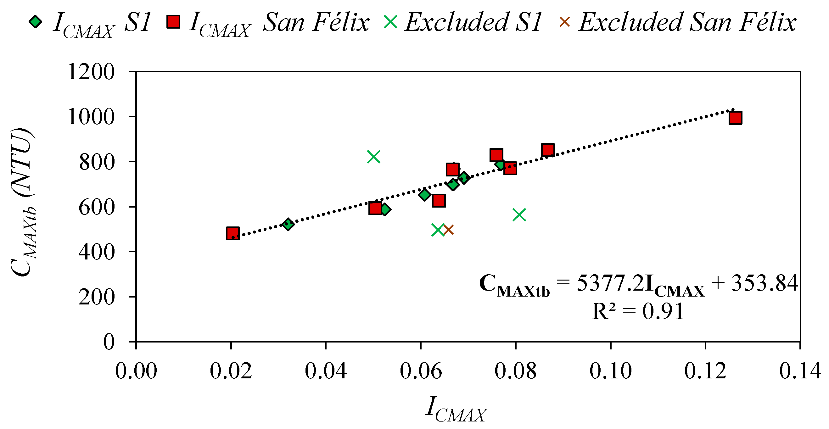
Figure 7 presents the values of I_CMAX, calculated by Equation (6) for each rainfall event, and the maximum of measured turbidity in each event, C_MAXtb. Most values fit around a line except four cases:

Figure 7. Linear adjustment of C_MAXtb with the prediction index I_CMAX.

(i)

S1_4: It is an episode with very low precipitation (3 mm). Thus, although the previous dry period is very extensive (24 days), the prediction index yields lower values of the maximum concentration.

(ii)

S1_9 and S1_10: The measured maximum concentration values are below the trend followed by the other data. The possible reason of this phenomenon seems to be related with the energy of both events. The rains on these two days are characterized by an average intensity of low precipitation (less than 1 mm/h), so that the catchment and the network were slowly washed.

(iii)

SF_8: It is similar to episode S1_4. The precipitation is very low (2.3 mm).

Those reasons justify discarding the four cases. The relationship between C_MAXtb and I_CMAX fit to a line with a correlation coefficient of R² = 0.91.

The fitted line of the adjustment between the maximum concentration index, I_CMAX, and the maximum concentration of turbidity, C_MAXtb, is given by a linear regression

$$C_{MAXtb}=5377.2I_{CMAX}+353.84$$

(8)

Table 1 summarizes the parameters presented in the literature to predict pollution. This manuscript proposes a new model to estimate C_MAXtb. Moreover, proposed methodology also allows estimating TPP from hydraulic and hydrological parameters.

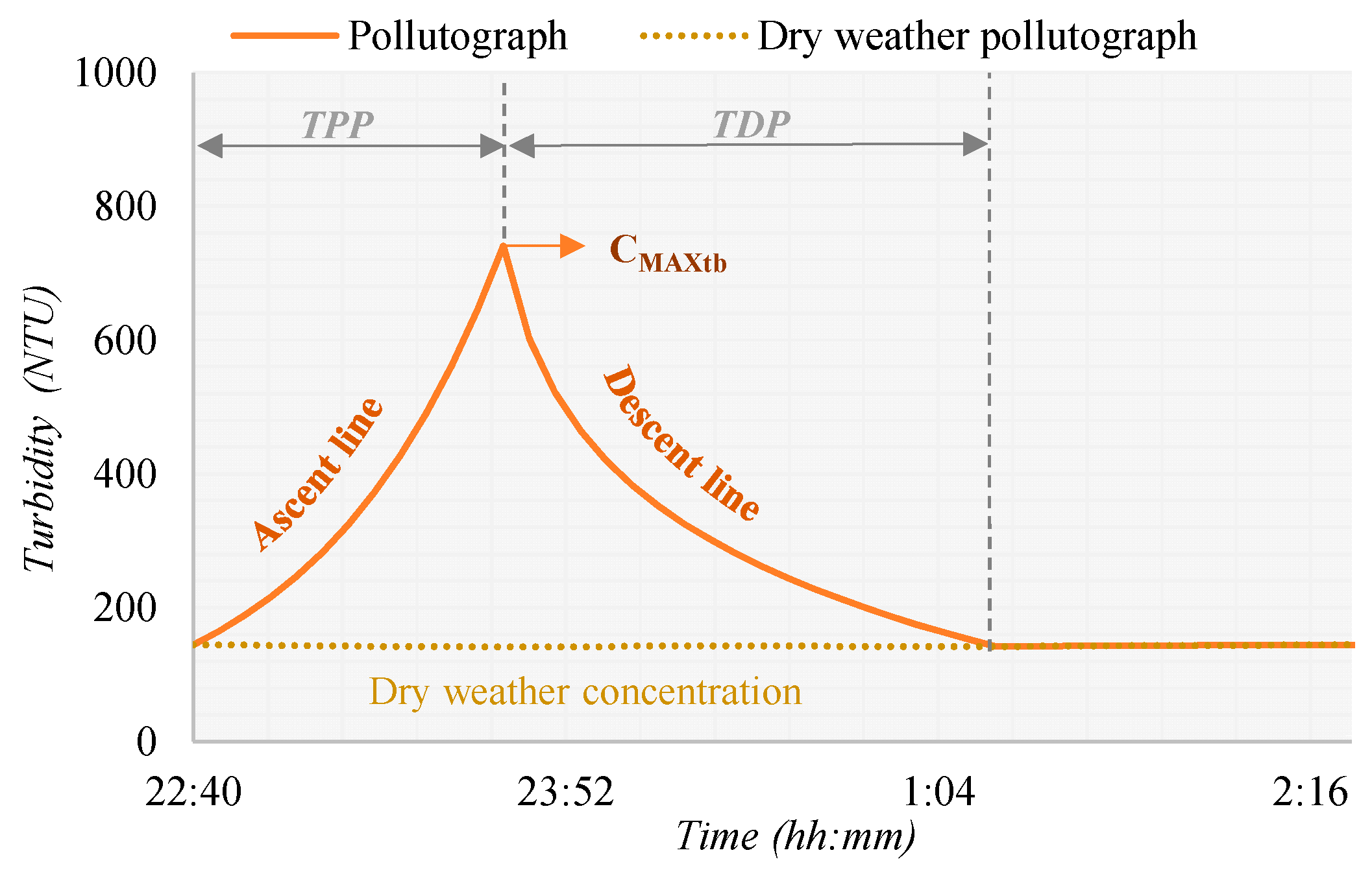
3.4. Development of Pollutographs from Prediction Indexes

Pollutograph is the representation of the concentration of a certain pollutant over time. The analysis of the ensemble formed by the hydrograph, the rainfall and the pollutograph of a given event can provide very important information about the mass mobilization of contaminants in an episode. For this reason, the knowledge of this graph is essential for the tasks of pollution management. Figure 8 presents a standard pollutograph.

Figure 8. Main parameters of a design pollutograph.

The line of ascent can be adjusted to the following exponential equation

$$C_a=a{b}^x=C_0{\left[{\left(\frac{C_{MAXtb}}{C_0}\right)}^{\frac{1}{N_a}}\right]}^n$$

(9)

where N_a is the number of intervals of 5 min in which the ascent time is divided; n indicates the interval (0 ≤ n ≤ N_a) in units of five minutes; and C_a and C₀ are the turbidity values at each interval n and at the beginning of the pollutograph, respectively (measured in NTU). The value of C₀ is assumed as the dry weather value at the beginning of the episode.

Once C_MAXtb and TPP have been calculated from prediction indexes, the time to the descent of pollutograph, TDP, can be defined as the time interval between the instant of the maximum concentration and the time when the concentration reaches dry weather values. The time to the descent of pollutograph value has been adjusted for each of the catchments showing a linear relationship with pollutograph time to the peak. The adjustment of TDP for each catchment is given by

$$\begin{array}{l}S1\to TDP=3.5TPP-125\\ SanFelix\to TDP=4.24TPP-40\end{array}$$

(10)

where TPP and TDP, in this equation, are expressed in minutes.

Differences between measured and calculated TDP at the studied events present average relative errors below 13% for the S1 catchment and 14% for the San Félix catchment.

The descent line of the pollutographs can be adjusted to a logarithmic function:

$$C_d=a\ln \left(x\right)+b=\left(\frac{C_{TStb}-C_{MAXtb}}{\ln \left(N_d-N_a+1\right)}\right)\ln \left(n-N_a+1\right)+C_{MAXtb}$$

(11)

where N_d is the number of intervals of five minutes in which the descent time is divided; n indicates the interval (N_a ≤ n ≤ N_d) in units of five minutes; and C_d and C_TStb are the turbidity values at each n interval and at the end of the event, corresponding to TDP time, respectively (measured in NTU). Equation (11), when n = N_a, ln(n − N_a + 1) = 0, and C_a = C_d = C_MAXtb, assures continuity.

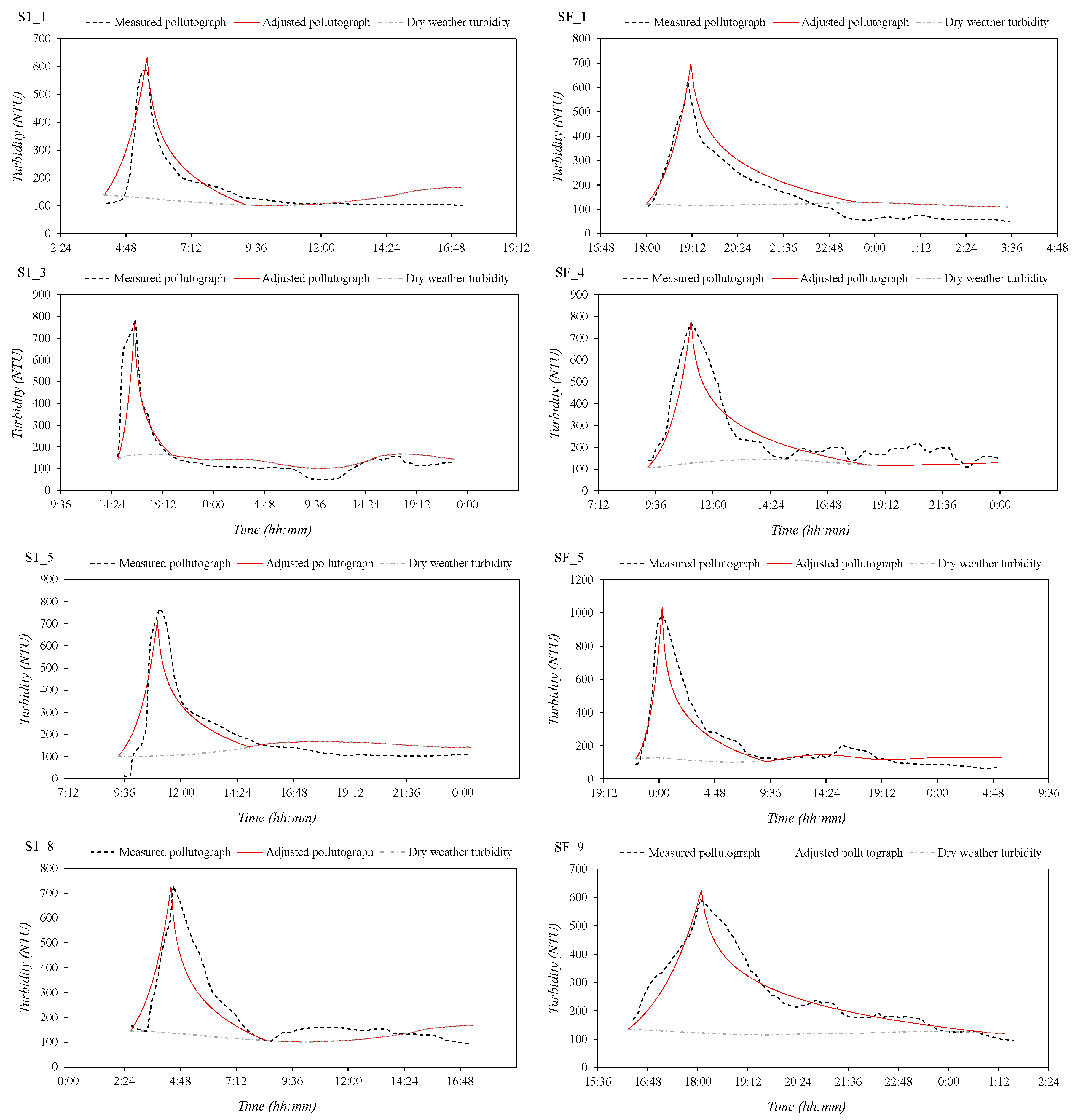
Figure 9 shows some of the measured pollutographs. They are compared with the pollutographs obtained by Equations (9)–(11). Results show a good agreement between measured and calculated pollutographs; therefore, the proposed methodology is suitable for estimating pollutographs from indexes.

Figure 9. Comparison between measured pollutographs and calculated ones through the suggested methodology.

Several multi-peaked hydrographs have been registered, however none of them led to a multi-peak pollutograph (see case S1_3 and San Felix _5 in Figure 5). Actually, the flushing produced by the first hydrograph peak leads to the removal of a second peak in the pollutograph. Present methodology also covers multi-peak hydrographs with unique pollutograph peak, according to observed events.

4. Conclusions

Time-continuous measurements of rainfall, in-sewer turbidity and water flow depth have been registered for almost two years. From the measurements, quality and hydraulic rainfall-event variables have been defined (Table 5 and Table 6).

In this paper, turbidity has been chosen as a pollutant indicator as other authors have pointed out it can be used in order to estimate different water quality parameters, e.g., TSS or COD, through on-site linear regressions.

The correlation between variables has been studied (Table 7 and Table 8). High correlations have been found between some of the analyzed variables, such as between the time to the peak of hydrograph, TPH, and the time to peak of pollutograph, TPP.

To improve those correlations, two prediction indexes have been suggested: the pollutograph time to the peak index, I_TPP, presented in Equation (4), and the maximum concentration index, I_CMAX, shown in Equation (6).

From the above prediction indexes, a statistical model has been proposed. This model allows estimating the time to peak of the pollutographs, TPP, presented in Equation (5), and the maximum values of turbidity, C_MAXtb, as seen in Equation (8).

The statistic model proposed has a high correlation for catchments S1 and San Felix in the city of Murcia. This model constitutes a useful tool for providing knowledge about pollutants transport in the combined sewer overflow in the city of Murcia. In fact, it can help, as an advisory tool, to support the design of CSO tanks or to forecast pollution risks for use within a CSO management strategy.

An application of the proposed model is the definition of pollutographs. In Figure 8, a standard pollutograph is shown. Pollutograph is modeled through the former index variables together with the pollutographs time to descent, TDP, proposed in Equation (10). Ascent and descent curves are proposed in Equations (9) and (11). Pollutographs estimated through this methodology agree reasonably well with the measured ones during the registered events (Figure 9). In this way, from a rainfall forecast, P_TOTAL, and other variables such as the dry weather period, DWP, and the time to peak of the hydrograph, pollutographs can be simulated for multiple prognosis scenarios. Thus, the methodology provides information of the pollution during wet weather in combined sewer systems.

Although this study is specific for these catchments, it may be used as a starting point for other catchments to establish effective policies for combined sewer overflow control. Moreover, the authors consider that extending the pollutographs to other catchments could lead to standardize the coefficients so that a “design pollutograph” can be defined and used as a reference for other studies.