Analysis of Coastline Extraction from Landsat-8 OLI Imagery

Abstract

Coastline extraction is a fundamental work for coastal resource management, coastal environmental protection and coastal sustainable development. Due to the free access and long-term record, Landsat series images have the potential to be used for coastline extraction. However, dynamic features of different types of coastlines (e.g., rocky, sandy, artificial), caused by sea level fluctuation from tidal, storm and reclamation, make it difficult to be accurately extracted with coarse spatial resolution, e.g., 30 m, of Landsat images. To access this problem, we analyze the performance of coastline extraction by integrating downscaling, pansharpening and water index approaches in increasing the accuracy of coastline extraction from the latest Landsat-8 Operational Land Imager (OLI) imagery. In order to prove the availability of the proposed method, we designed three strategies: (1) Strategy 1 uses the traditional water index method to extract coastline directly from original 30 m Landsat-8 OLI multispectral (MS) image; (2) Strategy 2 extracts coastlines from 15 m fused MS images generated by integrating 15 m panchromatic (PAN) band and 30 m MS image with ten pansharpening algorithms; (3) Strategy 3 first downscales the PAN band to a finer spatial resolution (e.g., 7.5 m) band, and then extracts coastlines from pansharpened MS images generated by integrating downscaled spatial resolution PAN band and 30 m MS image with ten pansharpening algorithms. Using the coastline extracted from ZiYuan-3 (ZY-3) 5.8 m MS image as reference, accuracies of coastlines extracted from MS images in three strategies were validated visually and quantitatively. The results show that, compared with coastline extracted directly from 30 m Landsat-8 MS image (strategy 1), strategy 3 achieves the best accuracies with optimal mean net shoreline movement (MNSM) of −2.54 m and optimal mean absolute difference (MAD) of 11.26 m, followed by coastlines extracted in strategy 2 with optimal MNSM of −4.23 m and optimal MAD of 13.54 m. Further comparisons with single-band thresholding (Band 6), AWEI, and ISODATA also confirmed the superiority of strategy 3. For the various used pansharpening algorithms, five multiresolution analysis MRA-based pansharpening algorithms are more efficient than the component substitution CS-based pansharpening algorithms for coastline extraction from Landsat-8 OLI imagery. Among the five MRA-based fusion methods, the coastlines extracted from the fused images generated by Indusion, additive à trous wavelet transform (ATWT) and additive wavelet luminance proportional (AWLP) produced the most accurate and visually realistic representation. Therefore, pansharpening approaches can improve the accuracy of coastline extraction from Landsat-8 OLI imagery, and downscaling the PAN band to finer spatial resolution is able to further improve the coastline extraction accuracy, especially in crenulated coasts.

1. Introduction

Coastline, the boundary of land and sea, is vulnerable to the natural processes, such as coastal erosion-accretion and sea level changes, and human activities. Coastline mapping and change detection are, therefore, becoming a fundamental work for coastal resource management, environmental protection of coastal zone and coastal sustainable development [1,2,3]. Traditional ground surveying is known as an important method to complete coastline maps [4]. However, transferring the information from grounding surveys and photographs to coastline maps is costly and time-consuming [4,5]. With the characteristics of macroscopic, real-time, dynamic and cost-effective, and a large range of spatial and temporal scales, remote sensing data is used widely for coastline mapping and change detection [4,6,7].

In general, the coastline extracted from remote sensing imagery with finer spatial resolution is more likely to achieve higher accuracy [8], and an increasing number of high spatial resolution remote sensing images were used for effective coastline extraction. For example, Bruno et al. [9] exploits SAR image to semi-automatic coastline extraction on a very popular beach in Apulia Region (Italy); Liu et al. [10] presents a segmentation-based image processing method to extracted coastline from LiDAR data. Di et al. [11] employed semi-automatic method based on mean shift segmentation algorithm and a local refinement process to extract coastlines from IKONOS image; Puissant et al. [12] extracted coastlines from Quickbird multispectral (MS) images by using mathematical morphology; Lira et al. [3] used digital aerial photographs and digital orthophotomaps to present the first systematic, national-scale and consistent long-term coastline evolution data of Portuguese mainland low-lying sandy coasts; Sekovski et al. [13] applied a WorldView-2 MS image to delineate coastline by integrating supervised and unsupervised classification methods. Although the high spatial resolution remote sensing images play a significant role in obtaining satisfactory result regarding coastline extraction, their applications for regional-scale mapping in certain areas would be cost-prohibitive [8,13]; moreover, the infrequent revisit coverage of high spatial resolution remote sensing images would make it a challenge to perform coastline extraction in large areas. Valentini [14] proposed a tool for automatic shoreline detection based on remote sensing video systems, which have both high temporal and spatial resolutions. With respect to traditional procedures, video systems are a low-coast method for long-term and continuous coastline monitoring [14], while the storage of continuous video streams for long periods is large.

An alternative remote sensing image used for coastline extraction is the popular Landsat series imagery, because of its free access, large revisit coverage and long-term data record [15]. In real applications, Landsat series images acquired from sensors of Landsat 1–3 Multi-spectral Scanner (MSS), Landsat 4–5 Thematic Mapper (TM), Landsat-7 Enhanced Thematic Mapper Plus (ETM+) and Landsat-8 Operational Land Imager (OLI) are useful data for extracting coastline [16]. Lira and Taborda [17] summarized the advances of coastline extraction from available free-access satellite imagery, and showed that the Landsat imagery offers the best compromise between potential and availability to understand coastal dynamic features. Chen et al. [18] used Landsat MSS and TM MS images to monitor coastline changes in Lingding Bay, and the coastline extends on a coastal stretch of approximately 6 km; Ekercin [19] collected Landsat MSS, TM and ETM+ images between 1975 and 2001 to perform coastline change analysis in a part of the Aegean Sea; Wang et al. [20] used Landsat MSS, TM, ETM+ and OLI images for coastline detection along Ningbo City from 1976 to 2015; Pardo-Pascual et al. [21] evaluated how the storms impact the sandy beaches and the beach recovery process by describing the coastline positions obtained from Landsat TM and ETM+. Coastlines with special characteristics, such as deltas, exhibit less change in position, and they could be monitored by low resolution of Landsat images, while the coastline of sandy areas with small beaches is difficult to be monitored by low resolution images.

The biggest challenge for applying Landsat series images on coastline extraction and monitoring is the limited spatial resolution (30 m) of MS image [22]. Pardo-Pascual et al. [23] proposed an automatic method to extract shorelines from Landsat TM and ETM+ with subpixel precision, where the RMSE obtained in shoreline location ranges from 4.69 to 5.47 m. As the nature beaches are always changing over time, Almonacid-Caballer et al. [24] applied the annual mean shoreline position extracted from Landsat images to largely decline the short-term variability of shoreline, and the extracted shorelines were biased from the seaward by around 4 to 5 m. Foody et al. [25] evaluated a soft classification method in mapping coastline from a degraded simulated Landsat imagery, and the result presented coastline obtained at subpixel scale and the RMSE was 2.25 m. While, these methods are always complex and difficult to be achieved in real application. In the processing, only spectral information of Landsat imagery was utilized and the improvement of accuracy is limited. Notably, besides the 30 m MS image, landsat-7 ETM+ and Landsat-8 OLI sensors simultaneously acquire the 15 m spatial resolution panchromatic (PAN) band. Motivated by this, it is of great interest to improve the coastline extraction accuracy from Landsat ETM+ and OLI images by adding spatial information of PAN band into MS bands. In fact, researchers have developed many algorithms to generate a fine spatial resolution MS image by combining PAN and MS bands, and this concept is known as pansharpening [26].

Pansharpening is a data fusion technique adding high spatial information of a PAN image into a coarse spatial resolution MS image, resulting in a sharpened MS image that has the same spatial resolution of the PAN image. In the process, pansharpening aims to increase the spatial resolution while simultaneously preserving the spectral feature of primary MS image [27,28], and it has been widely used for integrating Landsat ETM+ MS and PAN band to improve the land use/cover mapping, precision agriculture, pollution monitoring, forest resource inventory and urban areas mapping [29,30,31]. However, for Landsat ETM+ satellite sensor, an instrument malfunction occurred on 31 May 2003, with the result that all Landsat-7 scenes acquired since 14 July 2003 have been collected in “SLC-off” mode. The newly launched Landsat-8 OLI image provides seven MS bands with 30 m spatial resolution and a PAN band with 15 m spatial resolution [32]. This makes it readily to obtain a 15 m spatial resolution fused MS image by pansharpening the Landsat-8 30 m MS image and 15 m PAN band. It is noteworthy that the spatial resolution of the sharpened MS image, however, may still not be sufficient to provide subtle variability of coastline retreat and advance information. An alternative solution of this problem is to produce spatially sharpened image with finer spatial resolution beyond both of the Landsat-8 OLI MS and PAN bands [33,34]. For this case, the PAN band is first downscaled to a finer spatial resolution band, and then integrated into the original MS bands by using pansharpening algorithm to produce a finer spatial resolution sharpened MS image.

Once sharpened MS image has been generated, coastline extraction methods should be further applied to extract coastline from the MS image [35]. Previous studies [20,36,37,38,39,40] have proved that water index method has advantages of universality, user friendliness and low computation cost in coastline extraction, and the common used water index is the normalized difference water index (NDWI) proposed by McFeeters [39]. In this paper, downscaling, pansharpening and water index approaches were used to extract coastlines from Landsat-8 OLI imagery. To evaluate how pansharpening algorithms impact on coastline extraction from fused Landsat-8 MS image, ten popular pansharpening algorithms, including additive à trous wavelet transform (ATWT), additive wavelet luminance proportional (AWLP), Brovey transform (Brovey), Gram Schmidt (GS), high pass filtering (HPF), intensity-hue-saturation (IHS), additive injection model (Indusion), principal component analysis (PCA), partial replacement adaptive component substitution (PRACS) and smoothing-filter-based intensity modulation (SFIM), are used to produce sharpened MS images. Moreover, three strategies are devised to extract coastlines from Landsat-8 OLI imagery. Strategy 1 extracts coastline directly from original Landsat-8 OLI 30 m MS image, and it is a traditional widely used method [41]. Strategy 2 extracts coastlines from pansharpened 15 m MS images generated by integrating Landsat-8 OLI 15 m PAN band and 30 m MS image with different pansharpening algorithms. Strategy 3 first downscales the Landsat-8 OLI PAN band to a finer spatial resolution (e.g., 7.5 m) band, and then extracts coastlines from the fused MS images generated by integrating downscaled PAN band and original MS image with different pansharpening algorithms.

2. Study Area and Datasets

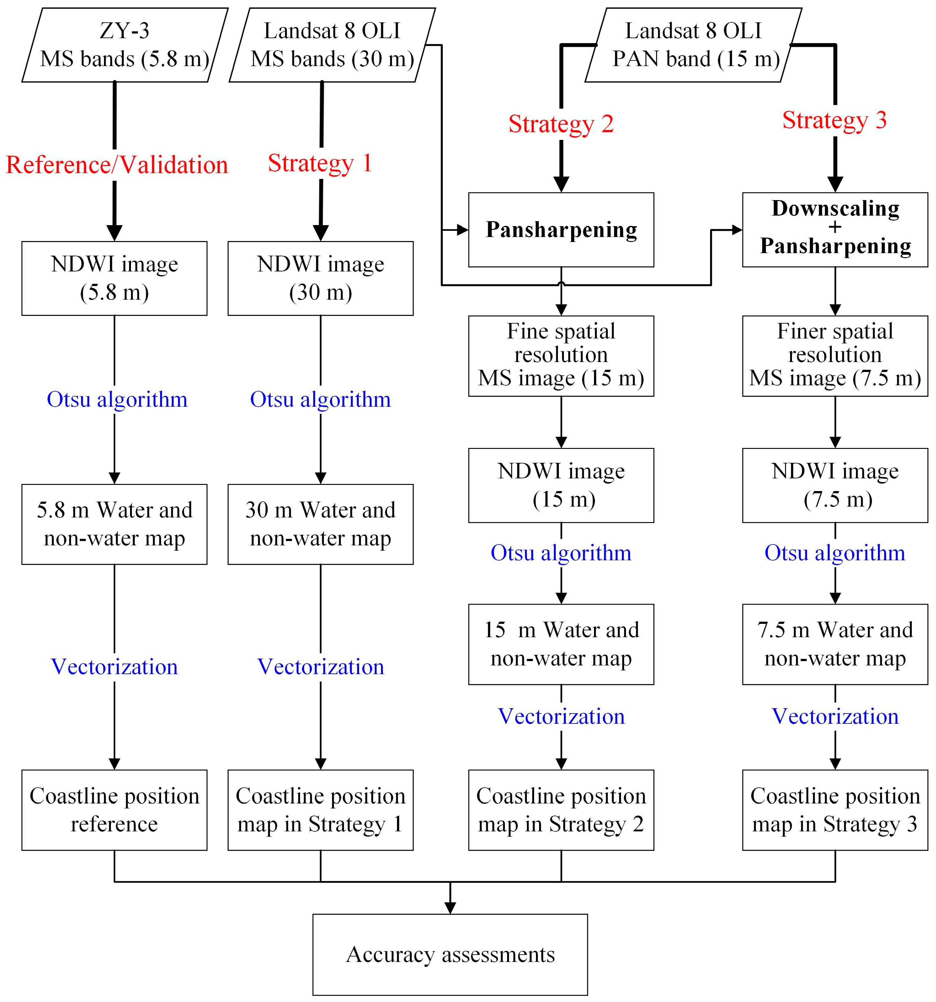
A portion of Ningbo coast was selected as the study area. As shown in Figure 1, Ningbo locates between 29°20′–29°32′ N and 121°50′–122°14′ E, and is next to the East China Sea. In China, Ningbo is an important port of international economic and cultural exchanges [42]. The increasing connection with the world has pushed the urban development of Ningbo, resulting in rapid coastline position changes during the past decades [20]. The types of Ningbo coast mainly contain bedrock coast, artificial coast and flat sandy coast. Subsites in Figure 1a presents two artificial coasts (subsites 1 and 4), two bedrock coasts (subsites 2 and 5) and two flat sandy coasts (subsites 3 and 6).

Figure 1. Geographical location of study area and the Landsat-8 OLI imagery: (a) multispectral (MS) image (R: band 5, G: band 4, B: band 3); (b–g) subsites 1–6 in turn.

In this study, one Landsat-8 OLI MS image (Figure 1a) and one PAN image, covering an area of 21 km × 21 km, were used for coastline extraction. The original Landsat-8 OLI imagery located in path 118 and row 039 was acquired at 2:24 a.m. (UTC) on 12 March 2015 and downloaded as the land surface reflectance product in the GeoTIFF format from United States Geological Survey (USGS) earth explore website (http://earthexplorer.usgs.gov/). Landsat-8 OLI imagery is with the Word Geodetic System (WGS84) datum and projected using the Universal Transverse Mercator (UTM) System. The detailed parameters of the Landsat-8 OLI imagery are presented in Table 1. Notably, the wavelength of PAN image only contains the spectral range from band 2 to band 4 of MS image, covering visible wavelengths, while the Landsat-7 ETM+ PAN band covers both visible and NIR wavelengths.

Table 1. Specifications of Landsat-8 OLI MS, PAN images and ZiYuan-3 surveying satellite (ZY-3) image.

Image Type	Acquisition Date	Spatial Resolution (m)	Bands	Wavelength (µm)
Landsat-8 OLI MS	12 March 2015	30	Band 1-coastal aerosol	0.43–0.45
			Band 2-blue	0.45–0.51
			Band 3-green	0.53–0.59
			Band 4-red	0.64–0.67
			Band 5-near infrared (NIR)	0.85–0.88
			Band 6-short wave infrared (SWIR 1)	1.57–1.65
			Band 7-short wave infrared (SWIR 2)	2.11–2.29
Landsat-8 OLI PAN	12 March 2015	15	Band 8-Panchromatic (PAN)	0.5–0.68
ZY-3	12 March 2015	5.8	Band 1-blue	0.45–0.52
			Band 2-green	0.52–0.59
			Band 3-red	0.63–0.69
			Band 4-NIR	0.77–0.89

Moreover, one ZiYuan-3 surveying satellite (ZY-3) MS image was used to extract the reference coastline covering the study area as shown in Figure 1. ZY-3 was launched on 9 January 2012, and it is China’s first civilian high-resolution stereo mapping satellite [43]. The MS image of ZY-3 has a spatial resolution of 5.8 m. The fine spatial resolution ZY-3 MS image was acquired at 2:45 a.m. (UTC) on 12 March 2015, which is really close to the acquisition time of Landsat-8 OLI imagery shown in Figure 1. In this case, tide difference can, therefore, be ignored for similar tide levels between Landsat-8 OLI and ZY-3 MS images [20]. Further information about the specifications of ZY-3 MS image is listed in Table 1.

For the acquired Landsat-8 OLI and ZY-3 MS images covering the same geographical region, ZY-3 MS image was first geometrically reprojected into the UTM, WGS84 coordinate system of Landsat-8 OLI image. Image-to-image registration method in ENVI 5.1 was then used to make pixels in the two images precisely coincide to the same points on the ground [27,44]. In the process, Landsat-8 PAN image was chosen as a master and ZY-3 was to be registered. The registration error was less than one pixel of ZY-3.

3. Methodology

In this study, three strategies were devised for the coastline extraction from Landsat-8 OLI MS and PAN bands. For strategy 1, the original Landsat-8 OLI MS bands were used directly to calculate the NDWI image, and then the dynamic segmentation method of Otsu algorithm [45] was used to separate the NDWI image into water and non-water features. The coastline was extracted finally by converting the water/non-water binary image into vector format with ArcGIS software. For strategy 2, instead of directly using Landsat-8 OLI MS image, pansharpening algorithms were first used to produce 15 m sharpened MS image by integrating Landsat-8 OLI MS and PAN bands, and then the fused MS image was used to calculate 15 m NDWI image and final coastline position map. For strategy 3, the 15 m PAN band was first downscaled to 7.5 m, and then pansharpening algorithms were used to produce 7.5 m sharpened MS image, which then was used to calculate 7.5 m NDWI image and final coastline position map. Downscaling method involved in the whole process of different strategies was performed via a polynomial kernel with 23 coefficients [46]. Ten pansharpening methods were collected to obtain the fine spatial resolution MS images in strategies 2 and 3. With respect to the accuracy assessment, the coastline derived from ZY-3 image with 5.8 m was regarded as reference. Specially, ZY-3 MS image was first used to calculate the 5.8 m NDWI image, and then Otsu segmentation method was applied to get the water/non-water binary map from 5.8 m NDWI, and the final reference coastline was extracted from the water/non-water binary map. The detailed methodology of the whole study is presented in Figure 2.

Figure 2. Flowchart of coastline extraction with three strategies.

3.1. Water Index

NDWI proposed by McFeeters (1996) is a non-linear conversion of the green and near-infrared band of MS image, and it is one of the most widely used water indices for coastline extraction. For water feature, it reflects the radiation in green band and absorbs in NIR band [35]. As for terrestrial vegetation and soil features, they have higher reflectance in NIR band than in green band. According to the different reflectivity between water and non-water, NDWI was defined as

$$\mathrm{NDWI}=\frac{{\rho }_{\mathrm{Green}}-{\rho }_{\mathrm{NIR}}}{{\rho }_{\mathrm{Green}}+{\rho }_{\mathrm{NIR}}}$$

(1)

where ${\rho }_{\mathrm{Green}}$ and ${\rho }_{\mathrm{NIR}}$ are the reflectance value of green and NIR band of MS image [39]. The results of the index can range from −1 to 1. Water surfaces tend to have positive values and non-water surfaces have negative values. In the case, MS image which has one green band and one NIR band can be used to calculate NDWI.

3.2. Water/Non-Water Binary Map Produced by Using Otsu Method

Once the NDWI image was produced, a threshold value is necessary to divide the image into two classes, land and water body. The problem is that the NDWI threshold value is not constant, but varies depending on the land cover components [47]. The Otsu method, proposed by Nobuyuki Otsu [45], selects an optimal threshold automatically from a gray image and the threshold maximize the inter-class discrepancy. Pervious researches have proved that Otsu method can successfully be applied to map water bodies from Landsat imagery [37,38].

Assuming t represents the threshold value, ranging from a to b ($-1\le a\le b\le 1$), the optimal threshold value t^* can be obtained by the following algorithm:

$$\{\begin{array}{l}{\sigma }^2=P_{\mathrm{nw}}\cdot {(M_{\mathrm{nw}}-M)}^2+P_{\mathrm{w}}\cdot {(M_{\mathrm{w}}-M)}^2\hfill \\ M=P_{\mathrm{nw}}\cdot M_{\mathrm{nw}}+P_{\mathrm{w}}\cdot M_{\mathrm{w}}\hfill \\ P_{\mathrm{nw}}+P_{\mathrm{w}}=1\hfill \\ t^{*}=\mathrm{Arg}\begin{array}{c}\underset{a\le t\le b}{\mathrm{Max}}\left\{P_{\mathrm{nw}}\cdot {(M_{\mathrm{nw}}-M)}^2+P_{\mathrm{w}}\cdot {(M_{\mathrm{w}}-M)}^2\right\},\end{array}\hfill \end{array}$$

(2)

where $\sigma$ is the inter-class variance of non-water and water pixels. $P_{\mathrm{nw}}$ is the possibility of a pixel belonging to the non-water and $P_{\mathrm{w}}$ means the possibility of a pixel that belongs to water. $M_{\mathrm{nw}}$ and $M_{\mathrm{w}}$ respectively represent the mean values of all non-water pixels and all water pixels, while $M$ is the mean value of the entire image. As a result, the pixels with values equal or higher the optimal threshold value was divided into water and scored 1. On the contrary, the pixel was classified as non-water and scored 0. The boundary of water and non-water is decided as coastline indicator.

3.3. Pansharpening Algorithms

Since the 1980s, studies on pansharpening with multiple source images for better understanding land surface feature has been conducted [48,49]. Many methods have been proposed to realize the fusion process and they can be classified into two categories: component substitution CS-based and multiresolution analysis MRA-based techniques [50]. In order to test the capability of pansharpening for coastline extraction from Landsat-8 OLI imagery, ten widely used standard pansharpening algorithms encompassing different concept were chosen. Specially, five CS-based pansharpening algorithms, including IHS, PCA, GS, Brovey, PRACS, and five MRA-based pansharpening algorithms, including HPF, SFIM, Indusion, ATWT, AWLP, are chosen in the study. The brief introduction of these pansharpening algorithms is described in the following subsections.

3.3.1. Intensity-Hue-Saturation (IHS)

The IHS transformation is a classic image fusion method and it is based on the component substitution to enhance the spatial feature of coarse spatial resolution MS image. Intensity refers to the total brightness of a color image, while hue specifies the dominant or average wavelength of light contributing to a color image and saturation indicates the purity of a color relative to gray [51]. Arbitrary bands of MS image assigned to RGB channel can be transformed to IHS space and replace the first band by PAN image with fine spatial resolution. Then, the substitutive IHS was transformed backward the original RGB space [52]. In the process, the IHS transformation method injects the spatial information of PAN image into MS image and preserves the spectral information of original MS image.

3.3.2. Principal Component Analysis (PCA)

The PCA method is widely used in signal processing, statistics and many other areas, and is also a classic image fusion method [27]. PCA transformation generates a set of uncorrelated components from original MS image. The first component contains the largest information of the color image, and the following ones compose the residual information decreasing successively. Theoretically, the largest information specifies the common feature in all bands, i.e., the spatial feature, while the unique spectral information was mapped to other components [27,53]. Similar to IHS, the first component was substituted by the fine resolution PAN image. Finally, an inverse PCA transform takes the fused image back into the original multispectral feature space [54].

3.3.3. Gram Schmidt (GS)

The widespread GS method was invented by Laben and Brover in 1998 and patented by Eastman Kodak [55]. The GS orthogonalizes the bands of MS image to remove redundant information from imputed coarse spatial resolution MS image [27]. By spatially averaging the multispectral MS bands, a coarse spatial resolution synthetic panchromatic band was generated and used as the first band of GS transform. Then the high spatial resolution PAN image replaces the first GS transform component. Finally, an inverse GS transformation is applied to produce the fine spatial resolution MS image [49].

3.3.4. Brovey Transform (Brovey)

The Brovey transform is a generally used method based on the chromaticity transform [56]. This algorithm considers that the image consists of two parts, hue and brightness [57]. First, each MS band that is chosen to compose a RGB space is divided by the sum of the three bands. The aim of the ratio is to preserve the spectral feature of coarse spatial resolution MS image. Second, multiplying the ratio by the high spatial resolution PAN band obtains the overall brightness of high spatial resolution image. Finally, a new image with the spatial resolution of inputted PAN image is produced. In the process, the Brovey transform technique provides excellent visually contrast of the fusion image.

3.3.5. Partial Replacement Adaptive Component Substitution (PRACS)

The PRACS method based on component substitute was proposed by Choi et al. (2011) [58] to improve the spatial and spectral quality of original MS imagery. To obtain the fine spatial resolution MS image, the method is organized into two steps. The first step is the construction of fine and coarse spatial resolution component images using PAN and MS images by partial replacement. Considering the unfixed relationship varying with different object, area, and circumstance, a linear regression algorithm is performed between PAN image and each MS bands. The second step is find an optimal CS fusion model to minimize the local and global spectral distortion between the PAN image and each MS band while preserving the spatial information within original PAN image [58].

3.3.6. High Pass Filtering (HPF)

The HPF method proposed by Schwengerdt (1980) is regarded as a predecessor of image fusion methods that are based on the concept of adding the spatial information extracted from fine spatial resolution image into the original coarse spatial resolution MS image [27,59]. For HPF, the spatial feature consists with the high frequency information, which can be obtained by filtering the PAN image with a high-pass filter or subtracting the low-pass filter image from the original PAN image. There are many types of filters that can be used in the process, such as Box and Gaussian filters. In this paper, the Box filter was used to realize high spatial resolution information extraction from PAN image, and the final sharpened MS image is produced by injecting the extracted high spatial information into all bands of the initial MS image.

3.3.7. Smoothing-Filter-Based Intensity Modulation (SFIM)

The SFIM is a simple spectral preservation fusion method and it is based on a simplified solar radiation and land surface reflection model [60]. The method was proposed by Liu (2000) [60], and simplified as:

$$I_{\mathrm{SFIM}}=\frac{I_{\mathrm{coarse}}{I}_{\mathrm{fine}}}{I_{\mathrm{mean}}}$$

(3)

where $I_{\mathrm{SFIM}}$ means the fused image by SFIM method, $I_{\mathrm{coarse}}$ is the coarse spatial resolution MS image and $I_{\mathrm{fine}}$ is the fine spatial resolution PAN image. $I_{\mathrm{mean}}$ is a smoothed image using spatially averaging filter over the fine spatial resolution PAN image. Notably, $I_{\mathrm{coarse}}$ and $I_{\mathrm{mean}}$ must have the same pixel size with $I_{\mathrm{fine}}$. In Equation (3), the ratio between $I_{\mathrm{fine}}$ and $I_{\mathrm{mean}}$ removes the spectral and topographical information of the fine spatial resolution PAN image and maintains the fine spatial resolution textures. Thus, the pansharpened MS image not only has fine spatial resolution textures of PAN image, but also highly preserves the spectral information of the coarse spatial resolution MS image [60,61,62].

3.3.8. Additive Injection Model (Indusion)

Indusion is proposed by Khan et al. [63] for dealing with the spectral distortion caused by inaccurately registration between PAN and downscaled MS image. The method uses Induction scaling method instead of the bicubic interpolation within SFIM fusion method to produce a better co-registered downscaled MS image. Furthermore, a pair of upscaling and downscaling filters is applied to extract high frequency information from PAN image, and then the extracted spatial information was injected into original MS image, finally producing a fine spatial resolution MS image.

3.3.9. Additive À Trous Wavelet Transform (ATWT)

The ATWT method was developed by Núñez et al. [64] for image fusion based on multiresolution wavelet decomposition. In the process of wavelet transform, “à trous” algorithm is applied to obtain a shift-invariant discrete wavelet decomposition for input image. The PAN image is decomposed to several wave planes, and then the wavelet planes including the fine spatial information of PAN image is directly added into the original MS image [64,65]. Each of the fused fine spatial resolution MS bands is finally obtained by the inverse wavelet transform.

3.3.10. Additive Wavelet Luminance Proportional (AWLP)

Similarly to ATWT, AWLP is also a multiresolution wavelet-based image fusion method. To obtain a shift-invariant discrete wavelet decomposition for input image, the same discrete algorithm of the wavelet transform is used. Instead of directly injecting high spatial information into original coarse spatial resolution MS image, AWLP first transforms the RGB components of MS image to IHS space, and then adds the spatial information of PAN image into the first component. Finally, the new IHS space is inversed back into RGB components to produce the fused fine spatial resolution MS image [64,66].

3.4. Downscaling Panchromatic (PAN) Band with Interpolation

Downscaling is a potential method in remote sensing that can produce finer spatial resolution imagery than input [67]. In this research, downscaling approach is used to estimate the finer spatial resolution PAN band $P^{15/s}$ from the observed PAN band $P^{15}$ with spatial scale $s$, and the process is formulated as

$$P^{15/s}=P^{15}{\downarrow }^s$$

(4)

where ${\downarrow }^s$ indicates a downscaling operation. Generally, it can be performed readily by a common interpolation method, such as bilinear and spline interpolations [67]. Bilinear, as an easy-to-operate method, was used in the paper.

3.5. Validation of Coastline Extraction

In order to have a quantitative assessment of the capacity of coastline extraction from Landsat-8 OLI imagery with different strategies, six indices, including mean absolute difference (MAD), maximum AD, minimum AD, mean net shoreline movement (MNSM), maximum positive NSM and maximum negative NSM were applied by using the coastline extracted from ZY-3 MS image as reference.

The Digital Shoreline Analysis System (DSAS) [68], a free extent for ArcGIS software, was applied in this study to determine the degree of position differences between extracted coastlines [69], such as NSM and AD. NSM represents a distance between the reference and the extracted coastline at each transect. The positive value of NSM means that the extracted coastline is on the sea side of the reference coastline; otherwise, the extracted coastline is on the land side. AD means the absolute distance between the extracted coastline and the reference coastline at each transect. In the test, AD value equals to the statistic of end point rate provided by DSAS at each transect. In the study, there are total of 866 transects that were created at a horizontal interval of 50 m to calculate the NSM and AD values.

4. Results

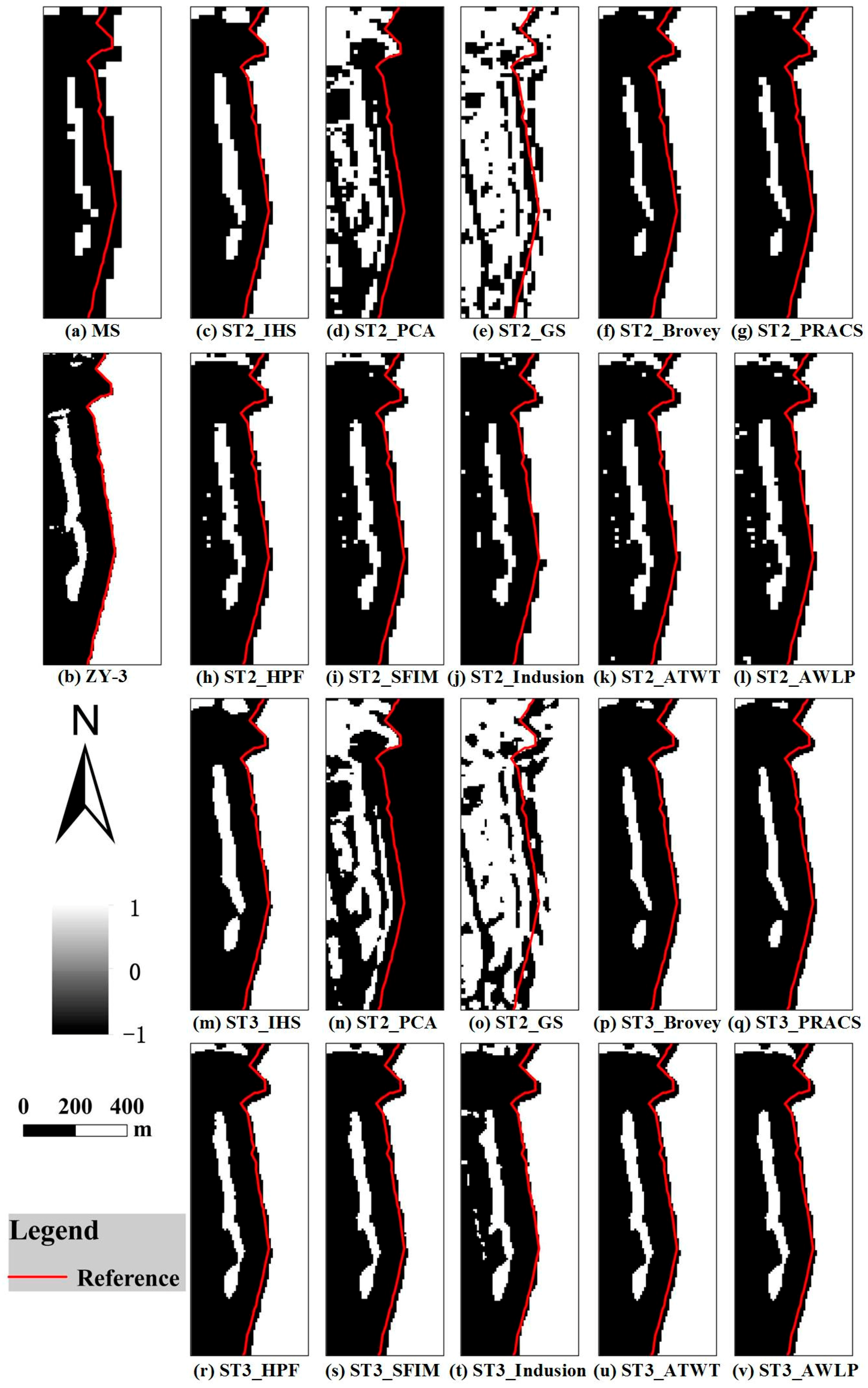
4.1. Pansharpened Multispectral (MS) Images

Ten pansharpening algorithms, including five CS-based methods of PCA, GS, IHS, Brovey, PRACS, and five MRA-based method of HPF, SFIM, Indusion, ATWT and AWLP, were used to produce sharpened MS images in strategies 2 and 3. Figure 3d–w present twenty fused MS images in standard false color at spatial resolutions of 15 m and 7.5 m. The original 30 m MS image, 15 m PAN band and 5.8 m ZY-3 MS image are also presented in Figure 3a–c. An artificial coastal subsite along the coastal is magnified 20 times and presents in lower-right corner of each fused MS images. In order to have a quantitative validation of the fused MS images generated by different pansharpening algorithms for strategies 2 and 3, the quality with no reference (QNR) index combined with the $D_s$ and $D_{\lambda }$ were applied in this subsection [70]. QNR, $D_s$ and $D_{\lambda }$ are widely used to examine the spectral and spatial information of the sharpened MS with no reference. Specially, $D_s$ is used to validate the spectral information inheriting from the original coarse spatial resolution MS image, and lower $D_s$ value means better maintaining of the original MS spectral information. $D_{\lambda }$ is used to validate the spatial information exploited from the fine spatial resolution PAN band, and lower $D_{\lambda }$ value indicates better restoring of the spatial information of PAN band. QNR is a combination of $D_s$ and $D_{\lambda }$, and higher value of QNR means better quality of the sharpened MS image.

Figure 3. The original Landsat MS image (a), 15 m PAN image (b), reference image (c) and fused MS images (d–w) produced in strategy (ST) 2 and ST 3. (R: NIR band, G: Red band, B: Green band).

In the section, a brief visual and quantitative analysis, including spectral preserving and spatial improvement, is presented. In Figure 3, compared with the original 30 m MS image shown in Figure 3a, the spatial detailed information in all fused images are improved obviously, practically in the results of strategy 3, which shows the promising advance of pansharpening algorithms. Compared with the results of most CS-based pansharpening algorithms, the results of MRA-based pansharpening algorithms of HPF, SFIM, Indusion, ATWT, AWLP can better preserve the spectral information within original 30 m MS image, and they achieve obvious lower $D_s$ values and higher QNR values for both strategies 2 and 3 as shown in Table 2. From Figure 3 and Table 2, the CS-based method of PRACS achieves the lowest $D_s$ and $D_{\lambda }$ values, and highest QNR values, and PCA and GS shows obviously spectral distortion. The colors of Sea are moorea blue in the original MS image, while that of PCA and GS fused MS images are cheery cola and medium azul, respectively. The colors of vegetation features in the fused PCA and GS images change from bright red to purple and black red, respectively. This is because PCA and GS algorithms have poor ability to preserve the spectral information of original MS image in the resultant sharpened MS image. Compared with strategy 2, most of the sharpened MS images in strategy 3 achieve an improvement of the QNR, $D_s$ and $D_{\lambda }$ values, and this indicates the superiority of strategy 3 in preserving spectral information of original MS image and exploiting spatial information of PAN band.

Table 2. $D_s$, $D_{\lambda }$ and QNR of the fused MS images generated by different pansharpening algorithms in strategy 2 (ST2) and strategy 3 (ST3).

Scheme	Fusion Methods	${\mathit{D}}_{\mathit{s}}$	${\mathit{D}}_{\mathit{\lambda }}$	QNR	Scheme	Fusion Methods	${\mathit{D}}_{\mathit{s}}$	${\mathit{D}}_{\mathit{\lambda }}$	QNR
Ideal value		0	0	1	Ideal value		0	0	1
ST 2	PCA	0.2803	0.1365	0.6214	ST 3	PCA	0.2594	0.1331	0.6421
	GS	0.2803	0.1365	0.6214		GS	0.1659	0.0798	0.7675
	IHS	0.2394	0.2030	0.6062		IHS	0.2298	0.2059	0.6116
	Brovey	0.2185	0.1728	0.6465		Brovey	0.2103	0.1733	0.6529
	PRACS	0.0588	0.0252	0.9175		PRACS	0.0689	0.0225	0.9101
	HPF	0.1489	0.1450	0.7277		HPF	0.1474	0.1299	0.7419
	SFIM	0.1483	0.1481	0.7256		SFIM	0.1405	0.1255	0.7516
	Indusion	0.0884	0.1084	0.8128		Indusion	0.0737	0.1595	0.7786
	ATWT	0.1770	0.1778	0.6766		ATWT	0.1749	0.1596	0.6933
	AWLP	0.1968	0.2051	0.6384		AWLP	0.1873	0.1793	0.6671

4.2. Coastline Extraction

Once the fused MS images in strategies 2 and 3 have been produced, they can thus be used to generate corresponding NDWI images, which are shown in Figure 4c–v. Moreover, by applying the Otsu segmentation method, the water and non-water binary maps shown in Figure 5 were generated from the NDWI images. It can be found that more spatial detail information is exploited within the NDWI images of strategies 2 and 3 by comparing with that of the original 30 m NDWI image (Figure 4a), and the corresponding water body maps of strategies 2 and 3 also have more spatially smooth boundaries than that of original 30 m water body map shown in Figure 5a. Compared with the results of strategy 2, the water body maps of strategy 3 contain more spatial details and have spatially smooth boundaries, which shows the efficiency of strategy 3 for coastline extraction. For both strategies 2 and 3, most of the water body maps of MRA-based pansharpening algorithms contain more spatial detail information than that of CS-based pansharpening algorithms. Meanwhile, in Figure 4 and Figure 5, the worst results are associated with the PCA and GS algorithms, and they are almost impossible to distinguish water and non-water features. This is because the fused MS images generated by PCA and GS have a serious spectral distortion of band 3 and band 5, making the calculated NDWI images have a confusion of water and non-water features, and this phenomenon can also be observed in Section 4.1. Although the exploiting of fine spatial information within PAN image is really important, the spectral preserving may be more important for the fused MS image to calculate NDWI image. In the following section, PCA and GS algorithms were, therefore, not applied to produce coastlines. Based on the water body maps shown in Figure 5, twenty vector coastlines were delineated with ArcGIS software. These coastlines were then used to calculate six accuracy indices mentioned in Section 3.5 by using the coastline extracted from the ZY-3 water body map as reference.

Figure 4. Normalized difference water index (NDWI) sub-images derived from original MS images and pansharpened MS images.

Figure 5. Classified water and non-water binary sub-maps using Otsu method.

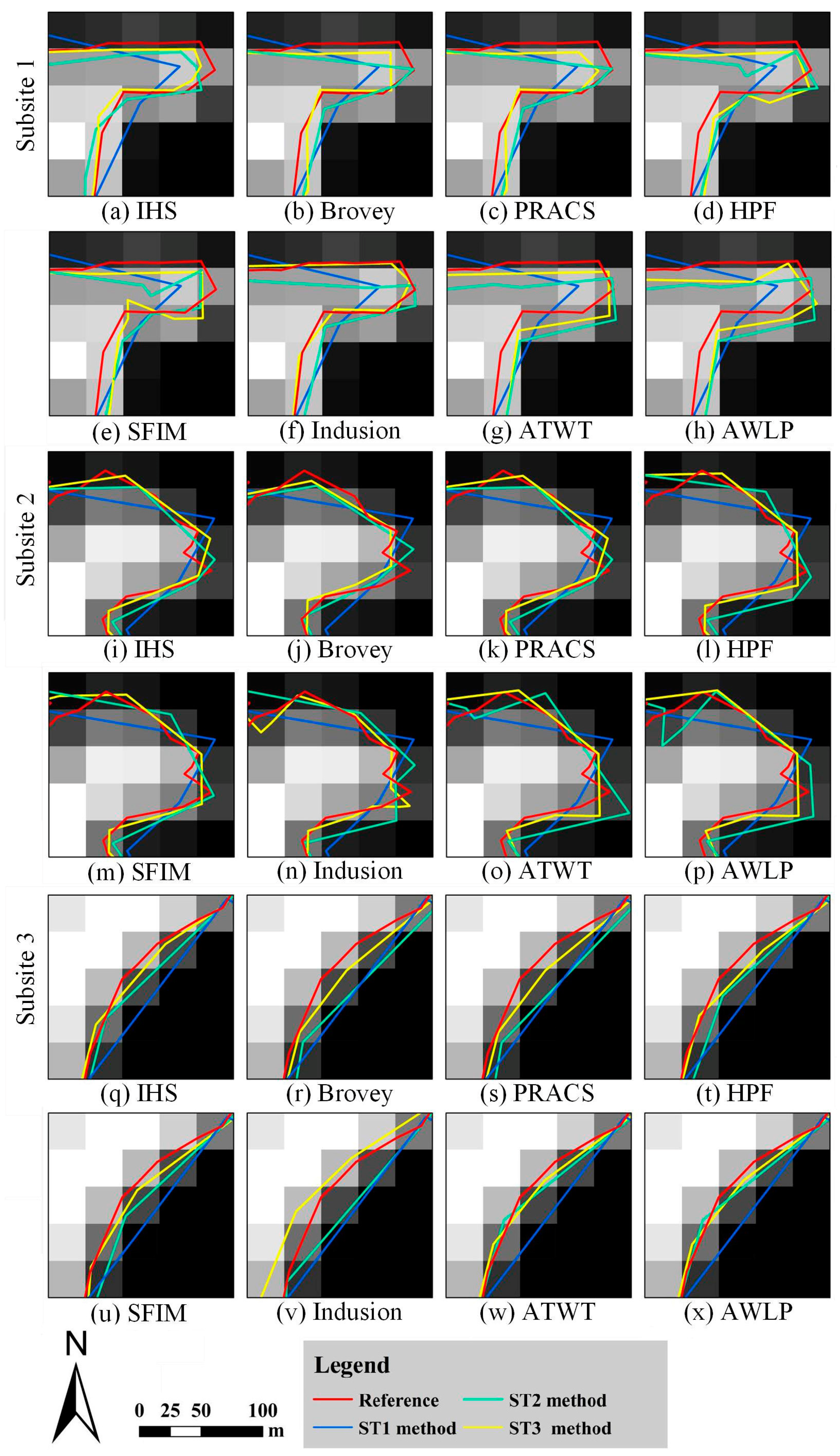
4.3. Comparising Extracted Coastlines of Different Strategies

To understand the capacity of coastline extraction from Landsat-8 OLI imagery with different strategies, three subsites containing artificial coast, bedrock coast and flat sandy coast, were chosen to analysis how the three strategies impact on the extraction accuracy of coastlines. From the results shown in Figure 6, it can be seen that the results produced in strategies 2 and 3 have better performance than that in strategy 1, and strategy 3 produces the best results. For subsite 1 (artificial coast), the coastlines derived from eight fusion methods in strategy 3 are closest to the reference coastline, followed by the coastline extracted in strategy 2. The coastline extracted from original 30 m MS image presents the largest difference with the reference coastline, and the maximum distance between actual coastline and reference almost reaches more than one pixel in horizon direction. For subsite 2 (bedrock coast), the coastline has twists and turns. It can be seen that the coastline in strategy 1 cannot fully reflect the sinuosity features of bedrock coastline. On the contrary, the coastlines produced in strategies 2 and 3 are able to represent the sinuosity features, and the coastlines in strategy 3 provide much more details about the twists and are the closest to the reference coastline. Coastlines as shown in Figure 6q–x are the results of sandy coast. The coastline of strategy 1 is overestimated by comparing with the reference coastline, and it is on the sea side and almost one pixel (30 m) away from the accurate coastline. It is observed that the coastlines derived from fused MS images of all pansharpening algorithms in strategy 3 present the best results that are approximate to the reference coastline.

Figure 6. The position of coastlines extracted from three different strategies for three subsites.

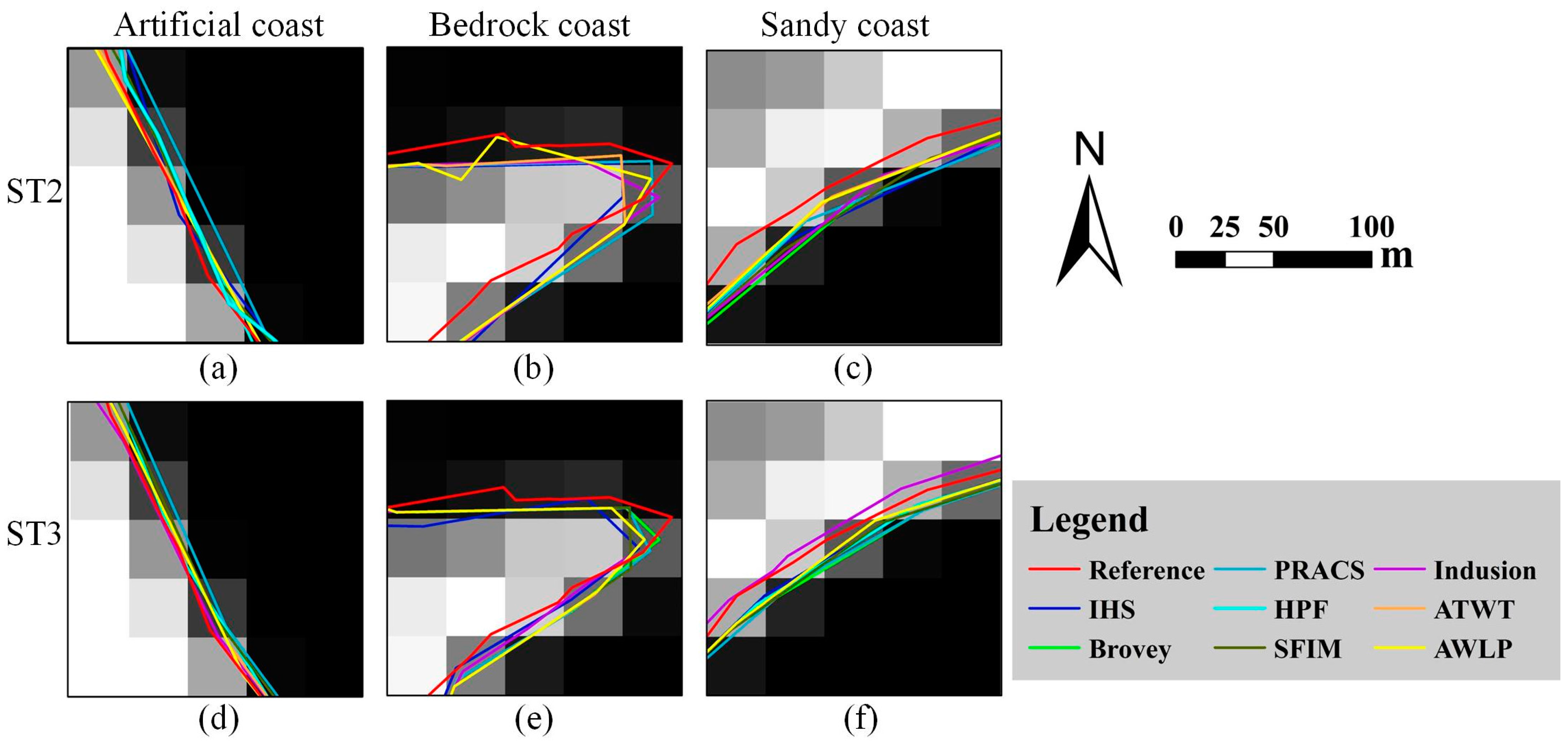
4.4. Comparising Extracted Coastlines of Different Pansharpening Algorithms

As presented in Section 4.2, eight fusion methods were finally applied for coastline extraction in strategies 2 and 3. In this section, we discussed the capacity of coastline extraction with the above eight pansharpening algorithms. Three subsites, referring to three different coast types, were shown in Figure 7, and the coastlines derived from different fused images are displayed with different colors. For the artificial coast shown in Figure 7a,d, the actual coastline refers to the boundary of construction and it tends to be a straight line. The results of different fusion methods agree well with the fluctuation trend of reference coastline. However, the coastlines of Brovey and PRACS algorithms are farther away from the reference coastline by comparing with the others, and they overlap with each other in both strategies 2 and 3. The coastlines of Indusion and AWLP in both strategies 2 and 3 are closer to the reference coastline than the others. For bedrock coast, as shown in Figure 7b,e, the coastlines extracted from Indusion images both in strategies 2 and 3 produced the most accurate and visually realistic presentation. For the sandy coast shown in Figure 7c,f, the coastline for ATWT in strategy 2 (see Figure 7c) is closest to the reference line, and the following is Indusion. In strategy 3 (see Figure 7f), the coastline extracted from the fused MS image of Indusion produced the most realistic and accurate representation, and the following are AWLP and ATWT.

Figure 7. The positions of coastlines extracted from ten different pansharpening algorithms for three subsites.

4.5. General Quantitative Analysis

Table 3 summarizes the coastline extraction accuracy for three strategies. As shown in Table 3 and Figure 8, coastline derived from the original MS image (strategy 1) has the worst accuracy index values by comparing with the extracted coastlines in strategies 2 and 3, which demonstrates the efficiency of pansharpening algorithms for coastline extraction from Landsat-8 OLI imagery. Comparing the MAD values in Table 3 and Figure 8a, the coastline extracted from original MS image has larger MAD value than that of strategies 2 and 3; moreover, it is observed that most of the coastlines extracted in strategy 3 have lower MAD values and maximum AD values than that of strategy 2. The coastline derived from HPF fusion image in strategy 3 has the lowest MAD value of 11.26 m, and followed by ATWT and PRACS. AWLP in strategy 3 achieves the lowest maximum AD value of 124.17 m, while its MAD value is 13.24 m. This demonstrates that strategy 3 has obvious advantage to extract coastlines with lower MAD values by comparing with that of strategies 2 and 1. For the minimum AD values, the coastline can keep very close to the reference coastline. There is no obvious difference between different pansharpening algorithms in the three strategies. Through the coastline extracted from the fused MS image produced by IHS has low minimum AD values, the maximum AD can reach 438.82 m in strategy 2 and 301.81 m in strategy 3. Therefore, it is not a stable algorithm used to extract coastline from Landat-8 OLI imagery.

Table 3. Summary of coastline extraction accuracy for different strategies and pansharpening algorithms. (MAD is short for mean absolute difference; MNSM is short for mean net shoreline movement).

Scheme	Fusion Methods	MAD (m)	Maximum AD (m)	Minimum AD (m)	MNSM (m)	Maximum Positive NSM (m)	Maximum Negative NSM (m)
ST 1	-	18.62	223.89	0.02	13.53	124.19	−223.89
ST 2	IHS	15.08	438.82	0.01	−4.23	40.00	−438.82
	Brovey	15.97	251.42	0.04	12.26	251.42	−108.6
	PRACS	16.16	222.95	0.04	12.41	136.75	−222.95
	HPF	14.31	137.19	0.02	10.25	137.19	−114.68
	SFIM	14.36	226.73	0.02	9.9	136.46	−109.53
	Indusion	13.54	227.08	0.01	9.21	129.47	−107.11
	ATWT	16.24	199.05	0	6.09	130.56	−106.84
	AWLP	16.42	198.67	0	6.13	128.99	−108.25
ST 3	IHS	12.3	301.81	0	−6.88	38.00	−301.81
	Brovey	12.02	128.58	0.01	8.36	128.58	−109.52
	PRACS	11.67	203.95	0.01	8.03	123.07	−203.95
	HPF	11.26	131.32	0.02	7.85	131.32	−106.64
	SFIM	11.99	133.15	0.06	8.66	133.15	−106.82
	Indusion	13.85	208.17	0.06	−2.54	122.74	−110.80
	ATWT	11.86	128.02	0.01	7.34	128.02	−106.46
	AWLP	13.24	124.17	0.01	4.78	124.17	−107.49

Figure 8. Mean absolute difference (MAD) and mean net shoreline movement (MNSM) values of the extracted coastlines from three different strategies with different pansharpening algorithms. The green lines, as contrasts, demonstrate the MAD value (a) and MNSM value (b) of coastline extracted in strategy 1.

Similar trend as that of MAD can also be observed for NSM index values shown in Table 3 and Figure 8b. For NSM, coastline produced in strategy 1 has the highest MNSM of 13.53 m. The coastlines extracted with different pansharpening algorithms in strategy 3 have lower MNSM values and maximum positive NSM values than the corresponding results in strategy 2. For the different pansharpening algorithms, it can be found that most of the MRA-based algorithms produce coastlines with lower MNSM values and maximum positive NSM values than that of CS-based pansharpening algorithms in both strategies 2 and 3. The Indusion in strategy 3 has the best MNSM value of −2.54 m by comparing with all of the other results, and the following is AWLP in strategy 3. Notably, three coastlines derived from IHS in strategy 2 and IHS, Indusion in strategy 3 have negative MNSM values, meaning that the coastlines move toward the land side of the reference coastline.

Figure 9 and Figure 10 shows coastline position differences of different MS images with respect to the transects from 270 to 340. The MEAN lines refer to the average value of all AD and NSM values of coastlines extracted by different pansharpening algorithms at each transect in strategies 2 and 3, respectively. In Figure 9 and Figure 10a,b, it can be seen that the position differences of coastlines in three strategies are mainly within a pixel (30 m) of the original MS image. The coastline in strategy 1 has a more significant position fluctuation than that in strategies 2 and 3. Moreover, both the position change fluctuations of AD and NSM in strategy 3 are slighter than that in strategy 2, which shows the superiority of strategy 3 by comparing with strategy 2. On the other hand, the extracted coastlines of different pansharpening algorithms in strategies 2 and 3 change on both sides of the reference coastline, while the MEAN lines change mainly on the ocean side of reference coastline.

Figure 9. Results of AD for different images from transect 270 to 340. (a) AD of strategy 2; (b) AD of strategy 3.

Figure 10. Results of figure for different images from transect 270 to 340 and the location of the transects. (a) NSM of strategy 2; (b) NSM of strategy 3; (c) position of selected transects.

To determine the potential use of coastline extracted with the integrated method, the histograms of NSM values (range from −30 m to 30 m) for the extracted coastlines with different methods are presented in Figure 11. For strategies 2 and 3, more than 94% of the NSM values are between −30 m and 30 m. Instead of using histogram, the NSM values of coastline extracted in strategy 1 was drawn as a polyline for better comparison. It can be found that the NSM values of coastline in strategy 1 disperses along the coastline but with an obvious seaward bias. For strategies 2 and 3, the central NSM values of the extracted coastlines gathered closer to the ideal value of 0. For example, the percentage of the NSM values between −12 m and 12 m in strategy 1 is 55.05%. However, for strategy 2, the maximum percentage is 78.13%, and the least is 61.58%. In strategy 3, the percentage of the NSM values between −12 m and 12 m can reach to 88.90%, and the least is 88.13%, which demonstrates the efficiency of strategy 3.

Figure 11. Histogram of NSM values of the extracted coastlines in strategy 1 (blue line), strategy 2 (red line) and strategy 3 (green line) with different methods: (a) IHS algorithm; (b) Brovey algorithm; (c) PRACS algorithm; (d) HPF algorithm; (e) SFIM algorithm; (f) Indusion algorithm; (g) ATWT algorithm; (h) AWLP algorithm.

4.6. Coastline Extraction Efectiveness

Based on quantitative and visual inspection of the resultant coastlines, it can be seen that the coastlines extracted in strategy 3 provide the most accurate and visually realistic representation, particularly for coasts with complex boundaries, such as bedrock coast. The following is the coastlines extracted in strategies 1 and 2. Increasing the spatial resolution of original MS image by directly using pansharpening algorithms or pansharpening with downscaled PAN image contributes to the accuracy increase of coastline extraction. With the increment of spatial resolution, a mixed pixel may be separated into two classes (water and non-water), and more details hidden in mixed pixels would be exploited in sharpened MS image. This is why coastlines extracted in strategy 3 are better than that in strategy 2. However, it cannot be concluded that with the continuing increase of spatial resolution of fused MS image, the resultant coastline would have continuous accuracy increase. For downscaling PAN band, the uncertainty would increase with the increment of spatial resolution of the downscaled PAN band by using spatial interpolation method.

In the study, ten pansharpening algorithms were used to produce fused image. Among the ten pansharpening algorithms, PCA and GS results have serious spectral distortions, which make them difficult to distinguish water and non-water from fused images. In general, water index is calculated based on spectral ratio and is sensitive to spectral distortion produced within the pansharpening process. CS-based pansharpening algorithms yield sharpened MS images by directly inject PAN band into original MS image, but often results in spectral distortion, whereas MRA approaches present less spectral distortion through a multiscale decomposition of PAN band into MS bands.

Comparing with all of the coastlines extracted from different pansharpening results in strategies 2 and 3, Indusion, ATWT and AWLP are the top three approaches. Instead of using spatial interpolation methods for downscaling original MS image, Induction scaling technique is used in Indusion pansharpening process for producing spectrally consistent downscaled MS image. For ATWT and AWLP, they use the “à trous” algorithm to produce a set of shift-invariant discrete wavelet planes with different degrees of spatial resolution, and additive method is applied to build a fused MS images. In wavelet-based image fusion process, the additive method preserves not only the high spatial information of PAN image but also all coarse spatial information of original MS image which is different from substitution method. In the condition, the ATWT and AWLP algorithms can sharpen the water and non-water boundaries, resulting in higher accuracy coastlines.

4.7. Threshold Value Effect on Coastline Extraction

The water index approach used in this study is based on the NDWI, and a key point is to generate water and non-water binary map from the NDWI image. Generally, the NDWI threshold value used to separate water and non-water features is not a constant value, and it varies depending on the land-cover components [47]. This is why the dynamic threshold selection method is needed for water and non-water features separation with NDWI image. Otsu method is a widely used dynamic threshold method to obtain optimal threshold from NDWI image by maximizing between the class various of water and non-water features [45]. For example, Du et al. [71] and Li et al. [38] have proved that the Otsu method can successfully be applied to map water bodies from Landsat imagery. In order to demonstrate the superiority of Otsu method against the constant threshold value of 0 in coastline extraction from Landsat-8 OLI imagery, the following example is presented. Specially, the subarea coastline extracted by using threshold of 0 is presented in Figure 12a, while Figure 12b shows the subarea coastline extracted with optimal threshold by applying Otsu method. Under the same condition, it can be seen that coastlines extracted with 0 threshold retreat toward land obviously and keep away from reference coastline, while that of Otsu is closer to the reference coastline. Moreover, for the whole study area shown in Figure 1, the MNSM of coastline extracted with threshold of 0 is −13.70 m and the MAD is 30.51 m, while that of Otsu result is 13.53 m (MNSM) and 18.62 m (MAD). Therefore, it is suggested to apply the Otsu method to extract coastline from Landsat-8 OLI imagery.

Figure 12. Positions of reference coastline (red line) and extracted coastline (blue line) from 30 m resolution Landsat image. Coastline in (a) extracted using 0 as the threshold, while Otsu method was used to obtain the optimal threshold in (b).

5. Discussions

Coastline extraction is important for the coastal management and coastline environment protection. The main limitations of coastline extraction from remote sensing image are the spatial resolution and cost. Landsat-8 OLI imagery is free access, but the spatial resolution limits the coastline extraction accuracy. Though several methods have been used and present in many previous research, automatic extraction method at subpixel level are difficult to understand and complex to implement. This study integrated pansharpening and water index approaches on Landsat-8 OLI imagery to discuss and analyze the ability of extracting coastline with higher accuracy. Pansharpening can take advantages of the fine spatial information within Landsat-8 OLI PAN band to increase the spatial resolution of original MS image, and water index was used to extract coastline from sharpened MS image.

5.1. Advance Accuracy Evaluation of the Proposed Method

To further evaluate the efficiency of various methods in coastline extraction, three original benchmark methods, including single-band thresholding (Band 6 for Landsat-8 OLI image) [72], classification (ISODATA) [35], water index (AWEI) [73], were used as the comparative methods against the method proposed in the paper. Table 4 shows the coastline extraction accuracy of three original methods. It can be found that the MNSM and MAD values of the three methods are stay at the high level, and much larger than that of strategies 2 and 3, especially the result of coastline extracted by AWEI method. This is because they are all based on the per-pixel scale (at spatial resolution of 30 m), while strategies 2 and 3 can take advantage of the PAN band to increase the accuracy of coastline extraction. In practice, there are many shortcomings of these methods, for example, AWEI combines all possible MS bands, which enhances the spectral characteristics of water and water-like features, but decrease the separability boundaries between them at the same time. On the contrary, single-band thresholding method cannot take full advantage of MS bands, and the extracted coastline position has a large fluctuation. For ISODATA method, the result is unstable, which is highly depends on the section of parameters during classification.

Table 4. Accuracy of three original benchmark methods in coastline extraction.

Other Methods	Band 6	AWEI	ISODATA
MNSM	11.29	36.67	14.43
MAD	23.99	44.58	24.12

5.2. Limitaions and Future Scopes

It is true that uncertainty would be inevitably introduced in the downscaling process, and this is a common but challenging issue in the field of image downscaling [67]. In fact, image downscaling is indeed an ill-posed problem, and the most challenging issue is to reduce the uncertainty [74]. During the past decades, the study of reducing the image downscaling uncertainty is mainly focused on two aspects. Firstly, using auxiliary data, such as multiple shifted images and digital elevation model, to increase the image downscaling accuracy. However, auxiliary data is not always available in real applications, and the collection of auxiliary data is always costly. Secondly, developing some powerful downscaling algorithms, such as machine learning based [75] and deep learning-based [76] approaches, to increase the image downscaling accuracy. In general, downscaling algorithms based on machine learning approaches are always mathematic complicated and time-consuming by comparing with normal image interpolation method. However, there is still of great interest for us to develop the machine learning-based downscaling algorithms, as it has achieved good performance in the field of image super-resolution. In future works, we would focus on the reducing of uncertainty of downscaling-based coastline extraction by proposing novel machine learning-based downscaling algorithms.

Although the coastline extracted from fused MS image have better accuracy, it is expected to add another Landsat OLI image acquired at different dates to prove that the proposed method can be replicated with success. Under this circumstance, we need to ensure that the reference coastline is obtained at almost the same time as that of Landsat OLI imagery, in which to eliminate the tide level difference between Landsat-8 OLI image and reference image. Although Landsat-8 OLI image is readily to be collected, the corresponding high spatial resolution remotely sensed image that used to extract reference coastline is always difficult to be obtained, and the high spatial resolution remotely sensed image, such as ZY-3, IKONOS and Quickbird, is often costly. We also considered to add more Landsat-8 OLI images to validate the performance of the proposed method, but for the study area, it is almost impossible for us to collect other high spatial resolution remotely sensed image that acquired at the same time of Landsat-8 OLI image. Notably, the aim of the paper is to confirm the availability of strategy 2 and strategy 3 and provide a reference for which algorithm is better in coastline extraction. It is, therefore, of great interest for us to apply more datasets and study areas to validate the performance and applicability of the methods in the future work.

Considering the results obtained, the coastline of coast with irregular shape, such as bedrock coast, is more sensitive to the spatial resolution of MS image, and further study should be done to analysis the relationship between the coast type and pansharpening algorithms. For further demonstrating the performance of pansharpening algorithms and downscaling method in coastline extraction, methods based on the integration of pansharpening and other water indices, such as MNDWI, are needed to discuss in the future.

6. Conclusions

The main purpose of this study was to discuss and analyze the capacity of coastline extraction from Landsat-8 OLI imagery by integrating pansharpening and water index (NDWI) approaches. Based on the spatial resolution of MS images used for coastline extraction, three strategies were proposed; moreover, ten popular pansharpening algorithms, including five CS-based and five MRA-based pansharpening algorithms, were used. From the above results analysis, it is reasonable to conclude that the proposed strategies 2 and 3 are efficient and readily methodologies that can be used for coastline extraction from Landsat-8 OLI imagery.

Specially, the conclusions for this study are summarized into five aspects:

(1)

For the fusion of Landsat-8 OLI original MS image and PAN band, PCA and GS pansharpening algorithms result in fused MS images with serious spectral distortions, and almost cannot be used to distinguish water and non-water features with NDWI and are also not suggested to be used for coastline extraction.

(2)

The coastlines produced in strategies 2 and 3 have better performance than that in strategy 1. With the increase of spatial resolution, subtle coastline changes which are indistinguishable in coarse spatial resolution MS images can be exploited well in the fused MS images in strategies 2 and 3. It indicates that pansharpening approach can improve the coastline extraction from Landsat-8 OLI imagery.

(3)

Strategy 3 produces coastlines with the best performance, indicating that further downscaling the PAN band is an alternative way to increase the coastline extraction accuracy.

(4)

For the ten widely used pansharpening algorithms, most of the MRA-based methods presents better results than that of CS-based methods in both strategies 2 and 3. Among the MRA-based methods, Indusion, ATWT and AWLP algorithms are the most efficient for increasing coastline extraction accuracy of Landsat-8 OLI imagery.

(5)

For the artificial coast, the coastlines extracted from most of the fusion methods agree well with the fluctuation trend of reference coastline. For both bedrock coast and sandy coast, the coastlines extracted from the fused images of Indusion algorithm in strategies 2 and 3 present the most accurate and visually realistic presentation.

References

- Aedla, R.; Dwarakish, G.S.; Reddy, D.V. Automatic shoreline detection and change detection analysis of Netravati-Gurpur River mouth using histogram equalization and adaptive thresholding techniques. Aquat. Procedia 2015, 4, 563–570. [Google Scholar] [CrossRef]
- Moore, L.J. Shoreline mapping techniques. J. Coast. Res. 2000, 16, 111–124. [Google Scholar]
- Lira, C.P.; Silva, A.N.; Taborda, R.; de Andrade, C.F. Coastline evolution of Portuguese low-lying sandy coast in the last 50 years: An integrated approach. Earth Syst. Sci. Data 2016, 8, 265–278. [Google Scholar] [CrossRef]
- Alesheikh, A.A.; Ghorbanali, A.; Nouri, N. Coastline change detection using remote sensing. Int. J. Environ. Sci. Technol. 2007, 4, 61–66. [Google Scholar] [CrossRef]
- Dewi, R.S.; Bijker, W.; Stein, A.; Marfai, M.A. Fuzzy classification for shoreline change monitoring in a part of the northern coastal area of Java, Indonesia. Remote Sens. 2016, 8, 190. [Google Scholar] [CrossRef]
- Li, W.; Gong, P. Continuous monitoring of coastline dynamics in western Florida with a 30-year time series of Landsat imagery. Remote Sens. Environ. 2016, 179, 196–209. [Google Scholar] [CrossRef]
- Boak, E.H.; Turner, I.L. Shoreline definition and detection: A review. J. Coast. Res. 2005, 21, 688–703. [Google Scholar] [CrossRef]
- Gens, R. Remote sensing of coastlines: Detection, extraction and monitoring. Int. J. Remote Sens. 2010, 31, 1819–1836. [Google Scholar] [CrossRef]
- Bruno, M.F.; Molfetta, M.G.; Mossa, M.; Nutricato, R.; Morea, A.; Chiaradia, M.T. Coastal observation through Cosmo-SkyMed high-resolution SAR images. J. Coast. Res. 2016, 33 Pt 2, 795–799. [Google Scholar] [CrossRef]
- Liu, H.; Wang, L.; Sherman, D.J.; Wu, Q.; Su, H. Algorithmic foundation and software tools for extracting shoreline features from remote sensing imagery and LiDAR data. J. Geogr. Inf. Syst. 2011, 3, 99–119. [Google Scholar] [CrossRef]
- Di, K.; Wang, J.; Ma, R.; Li, R. Automatic Shoreline Extraction from High-Resolution IKONOS Satellite Imagery. In Proceedings of the ASPRS 2003 Annual Conference, Anchorage, AK, USA, 5–9 May 2003. [Google Scholar]
- Puissant, A.; Lefevre, S.E.B.; Weber, J. Coastline Extraction in VHR Imagery Using Mathematical Morphology with Spatial and Spectral Knowledge. In Proceedings of the SPRS Congress Beijing 2008, Beijing, China, 3–11 July 2008; pp. 1305–1310. [Google Scholar]
- Sekovski, I.; Stecchi, F.; Mancini, F. Image classification methods applied to shoreline extraction on very high-resolution multispectral imagery. Int. J. Remote Sens. 2014, 10, 3556–3578. [Google Scholar] [CrossRef]
- Valentini, N.; Saponieri, A.; Molfetta, M.G.; Damiani, L. New algorithms for shoreline monitoring from coastal video systems. Earth Sci. Inf. 2017, 1–12. [Google Scholar] [CrossRef]
- Cohen, W.B.; Goward, S.N. Landsat’s role in ecological applications of remote sensing. BioScience 2004, 54, 535–545. [Google Scholar] [CrossRef]
- Sánchez-García, E.; Pardo-Pascual, J.E.; Balaguer-Beser, A.; Almonacid-Caballer, J. Analysis of the shoreline Position Extracted from Landsat TM and ETM+ Imagery. In Proceedings of the 36th International Symposium on Remote Sensing of Environmen, Berlin, Germany, 11–15 May 2015; pp. 991–998. [Google Scholar]
- Lira, C.; Taborda, R. Advances in applied remote sensing to coastal environments using free satellite imagery. In Remote Sensing and Modeling; Finkl, C.W., Makowski, C., Eds.; Springer International Publishing: Cham, Switzerland, 2014; Volume 9, pp. 77–102. ISBN 978-3-319-06325-6. [Google Scholar]
- Chen, S.; Chen, L.; Liu, Q.; Li, X.; Tan, Q. Remote sensing and GIS-based integrated analysis of coastal changes and their environmental impacts in Lingding Bay, Pearl River Estuary, South China. Ocean Coast. Manag. 2005, 48, 65–83. [Google Scholar] [CrossRef]
- Ekercin, S. Coastline change assessment at the Aegean Sea coasts in Turkey using multitemporal Landsat imagery. J. Coast. Res. 2007, 23, 691–698. [Google Scholar] [CrossRef]
- Wang, X.; Liu, Y.; Ling, F.; Liu, Y.; Fang, F. Spatio-Temporal change detection of Ningbo coastline using Landsat time-series images during 1976–2015. ISPRS Int. J. Geo-Inf. 2017, 6, 68. [Google Scholar] [CrossRef]
- Pardo-Pascual, J.E.; Almonacid-Caballer, J.; Ruiz, L.A.; Palomar-Vázquez, J.; Rodrigo-Alemany, R. Evaluation of storm impact on sandy beaches of the Gulf of Valencia using Landsat imagery series. Geomorphology 2014, 214, 388–401. [Google Scholar] [CrossRef]
- Liu, Q.; Trinder, J.; Turner, I.L. Automatic super-resolution shoreline change monitoring using Landsat archival data: A case study at Narrabeen–Collaroy Beach, Australia. J. Appl. Remote Sens. 2017, 11, 016036. [Google Scholar] [CrossRef]
- Pardo-Pascual, J.E.; Almonacid-Caballer, J.; Ruiz, L.A.; Palomar-Vázquez, J. Automatic extraction of shorelines from Landsat TM and ETM+ multi-temporal images with subpixel precision. Remote Sens. Environ. 2012, 123, 1–11. [Google Scholar] [CrossRef]
- Almonacid-Caballer, J.; Sánchez-García, E.; Pardo-Pascual, J.E.; Balaguer-Beser, A.A.; Palomar-Vázquez, J. Evaluation of annual mean shoreline position deduced from Landsat imagery as a mid-term coastal evolution indicator. Mar. Geol. 2016, 372, 79–88. [Google Scholar] [CrossRef]
- Foody, G.M.; Muslim, A.M.; Atkinson, P.M. Super-resolution mapping of the waterline from remotely sensed data. Int. J. Remote Sens. 2005, 26, 5381–5392. [Google Scholar] [CrossRef]
- Aiazzi, B.; Baronti, S.; Selva, M. Improving component substitution pansharpening through multivariate regression of MS+PAN data. IEEE Trans. Geosci. Remote Sens. 2007, 45, 3230–3239. [Google Scholar] [CrossRef]
- Amro, I.; Mateos, J.; Vega, M.; Molina, R.; Katsaggelos, A.K. A survey of classical methods and new trends in pansharpening of multispectral images. EURASIP J. Adv. Signal Process. 2011, 2011, 79. [Google Scholar] [CrossRef]
- Zhang, Y. Recent advances in pansharpening and key problems in applications. Int. J. Image Data Fusion 2014, 5, 175–195. [Google Scholar]
- Medina, A.; Marcello, J.; Rodriguez, D.; Eugenio, F.; Martin, J. Quality Evaluation of Pansharpening Techniques on Different Land Cover Types. In Proceedings of the IEEE International Geoscience and Remote Sensing Symposium, Munich, Germany, 2 August 2012; pp. 5442–5445. [Google Scholar]
- Lwin, K.K.; Murayama, Y. Evaluation of land cover classification based on multispectral versus pansharpened Landsat ETM+ imagery. GISci. Remote Sens. 2013, 50, 458–472. [Google Scholar]
- Wunderle, A.L.; Franklin, S.E.; Guo, X.G. Regenerating boreal forest structure estimation using SPOT-5 PAN-sharpened imagery. Int. J. Remote Sens. 2007, 28, 4351–4364. [Google Scholar] [CrossRef]
- Song, J.J.; Hun, C.J. Application effect analysis of image fusion methods for extraction of shoreline in coastal zone using Landsat ETM. Atmos. Ocean. Sci. 2016, 1, 1–6. [Google Scholar]
- Atkinson, P.M.; Pardo-Iguzquiza, E.; Chica-Olmo, M. Downscaling cokriging for super-resolution mapping of continua in remotely sensed images. IEEE Trans. Geosci. Remote 2008, 46, 573–580. [Google Scholar] [CrossRef]
- Wang, Q.; Shi, W.; Atkinson, P.M.; Pardo-Igúzquiza, E. A new geostatistical solution to remote sensing image downscaling. IEEE Trans. Geosci. Remote 2015, 54, 1–11. [Google Scholar] [CrossRef]
- Mitra, S.S.; Mitra, D.; Santra, A. Performance testing of selected automated coastline detection techniques applied on multispectral satellite imageries. Earth Sci. Inf. 2017, 10, 321–330. [Google Scholar] [CrossRef]
- Cui, B.; Li, X. Coastline change of the Yellow River estuary and its response to the sediment and runoff (1976–2005). Geomorphology 2011, 127, 32–40. [Google Scholar] [CrossRef]
- Du, Z.; Li, W.; Zhou, D.; Tian, L.; Ling, F.; Wang, H.; Gui, Y.; Sun, B. Analysis of Landsat-8 OLI imagery for land surface water mapping. Remote Sens. Lett. 2014, 5, 672–681. [Google Scholar] [CrossRef]
- Li, W.; Du, Z.; Ling, F.; Zhou, D.; Wang, H.; Gui, Y.; Sun, B.; Zhang, X. A comparison of land surface water mapping using the normalized difference water index from TM, ETM+ and ALI. Remote Sens. 2013, 5, 5530–5549. [Google Scholar] [CrossRef]
- Mcfeeters, S.K. The use of the normalized difference water index (NDWI) in the delineation of open water features. Int. J. Remote Sens. 1996, 17, 1425–1432. [Google Scholar] [CrossRef]
- Xu, H. A study on information extraction of water body with the modified normalized difference water index (MNDWI). J. Remote Sens. 2005, 5, 589–595. (In Chinese) [Google Scholar]
- Malahlela, O.E. Inland waterbody mapping: Towards improving discrimination and extraction of inland surface water features. Int. J. Remote Sens. 2016, 37, 4574–4589. [Google Scholar] [CrossRef]
- Yang, H. Definition of the management boundary between river and sea in Ningbo. J. Mar. Sci. 2009, 27, 64–75. (In Chinese) [Google Scholar]
- Wang, T.; Zhang, G.; Li, D.; Tang, X.; Jiang, Y.; Pan, H.; Zhu, X.; Fang, C. Geometric accuracy validation for ZY-3 satellite imagery. IEEE Geosci. Remote Sens. Lett. 2014, 11, 1168–1171. [Google Scholar] [CrossRef]
- Yang, C.; Cai, X.; Wang, X.; Yan, R.; Zhang, T.; Zhang, Q.; Lu, X. Remotely sensed trajectory analysis of channel migration in Lower Jingjiang Reach during the period of 1983–2013. Remote Sens. 2015, 7, 16241–16256. [Google Scholar] [CrossRef]
- Otsu, N. A threshold selection method from gray-level histograms. Automatica 1975, 11, 23–27. [Google Scholar] [CrossRef]
- Vivone, G.; Alparone, L.; Chanussot, J.; Dalla Mura, M.; Garzelli, A.; Licciardi, G.A.; Restaino, R.; Wald, L. A critical comparison among pansharpening algorithms. IEEE Trans. Geosci. Remote 2015, 53, 2565–2586. [Google Scholar] [CrossRef]
- Ji, L.; Zhang, L.; Wylie, B. Analysis of dynamic thresholds for the normalized difference water index. Photogramm. Eng. Remote Sens. 2009, 75, 1307–1317. [Google Scholar] [CrossRef]
- Sidek, O.; Quadri, S.A. A review of data fusion models and systems. Int. J. Image Data Fusion 2012, 3, 3–21. [Google Scholar] [CrossRef]
- Ehlers, M.; Klonus, S.; Johan Strand, P.R.; Rosso, P. Multi-sensor image fusion for pansharpening in remote sensing. Int. J. Image Data Fusion 2010, 1, 25–45. [Google Scholar] [CrossRef]
- Aiazzi, B.; Baronti, S.; Lotti, F.; Selva, M. A comparison between global and context-adaptive pansharpening of multispectral images. IEEE Geosci. Remote Sens. 2009, 6, 302–306. [Google Scholar] [CrossRef]
- Carper, W.J. The use of intensity-hue-saturation transformations for merging spot panchromatic and multispectral image data. Photogramm. Eng. Remote Sens. 1990, 56, 459–467. [Google Scholar]
- Tu, T.M.; Huang, P.S.; Hung, C.L.; Chang, C.P. A fast intensity-hue-saturation fusion technique with spectral adjustment for IKONOS imagery. IEEE Geosci. Remote Sens. 2004, 1, 309–312. [Google Scholar] [CrossRef]
- Wang, Z.; Ziou, D.; Armenakis, C.; Li, D. A comparative analysis of image fusion methods. IEEE Trans. Geosci. Remote Sens. 2005, 43, 1391–1402. [Google Scholar] [CrossRef]
- Psjr, C.; Sides, S.C.; Anderson, J.A. Comparison of three different methods to merge multiresolution and multispectral data: Landsat TM and SPOT panchromatic. Photogramm. Eng. Remote Sens. 1990, 57, 265–303. [Google Scholar]
- Laben, C.A.; Brower, B.V. Process for Enhancing the Spatial Resolution of Multispectral Imagery Using Pan-Sharpening. U.S. Patent 6,011,875, 4 January 2000. [Google Scholar]
- Gillespie, A.R.; Kahle, A.B.; Walker, R.E. Color enhancement of highly correlated images. II. Channel ratio and “chromaticity” transformation techniques. Remote Sens. Environ. 1987, 22, 343–365. [Google Scholar] [CrossRef]
- Xu, H. Study on data fusion and classification of Landsat 7 ETM+ imagery. Int. J. Remote Sens. 2005, 9, 186–194. (In Chinese) [Google Scholar]
- Choi, J.; Yu, K.; Kim, Y. A new adaptive component-substitution-based satellite image fusion by using partial replacement. IEEE Trans. Geosci. Remote Sens. 2011, 49, 295–309. [Google Scholar] [CrossRef]
- Aiazzi, B.; Alparone, L.; Baronti, S.; Garzelli, A. Context-driven fusion of high spatial and spectral resolution images based on oversampled multiresolution analysis. IEEE Trans. Geosci. Remote Sens. 2002, 40, 2300–2312. [Google Scholar] [CrossRef]
- Liu, J.G. Smoothing filter-based intensity modulation: A spectral preserve image fusion technique for improving spatial details. Int. J. Remote Sens. 2000, 21, 3461–3472. [Google Scholar] [CrossRef]
- Xu, R.; Xu, H. Evaluation on image fusion algorithms of Landsat-7 ETM+ PAN band and multispectral bands. Geo-Inf. Sci. 2004, 6, 99–103. (In Chinese) [Google Scholar]
- Liu, J.G. Evaluation of landsat-7 ETM+ panchromatic band for image fusion with multispectral bands. Nat. Resour. Res. 2000, 9, 269–276. [Google Scholar] [CrossRef]
- Khan, M.M.; Chanussot, J.; Condat, L.; Montanvert, A. Indusion: Fusion of multispectral and panchromatic images using the induction scaling technique. IEEE Geosci. Remote Sens. 2008, 5, 98–102. [Google Scholar] [CrossRef]
- Nunez, J.; Otazu, X.; Fors, O.; Prades, A.; Palà, V.; Arbiol, R. Multiresolution-based image fusion with additive wavelet decomposition. IEEE Trans. Geosci. Remote Sens. 1999, 37, 1204–1211. [Google Scholar] [CrossRef]
- Vivone, G.; Restaino, R.; Dalla Mura, M.; Licciardi, G. Contrast and error-based fusion schemes for multispectral image pansharpening. IEEE Geosci. Remote Sens. 2014, 11, 930–934. [Google Scholar] [CrossRef]
- Otazu, X.; Gonzalez-Audicana, M.; Fors, O.; Nunez, J. Introduction of sensor spectral response into image fusion methods. Application to wavelet-based methods. IEEE Trans. Geosci. Remote Sens. 2005, 43, 2376–2385. [Google Scholar] [CrossRef]
- Atkinson, P.M. Downscaling in remote sensing. Int. J. Appl. Earth Obs. Geoinf. 2013, 22, 106–114. [Google Scholar] [CrossRef]
- Thieler, E.R.; Himmelstoss, E.A.; Zichichi, J.L.; Ergul, A. The digital shoreline analysis system (DSAS) version 4.0-An ArcGIS extension for calculating shoreline change. In Open-File Report 2008-1278; Updated for Version 4.3; U.S. Geological Survey: Woods Hole, MA, USA, 2009; pp. 1–81. [Google Scholar]
- Zhang, T.; Yang, X.; Hu, S.; Su, F. Extraction of coastline in aquaculture coast from multispectral remote sensing images: Object-based region growing integrating edge detection. Remote Sens. 2013, 5, 4470–4487. [Google Scholar] [CrossRef]
- Alparone, L.; Aiazzi, B.; Baronti, S.; Garzelli, A.; Nencini, F.; Selva, M. Multispectral and panchromatic data fusion assessment without reference. Photogramm. Eng. Remote Sens. 2008, 74, 193–200. [Google Scholar] [CrossRef]
- Du, Y.; Zhang, Y.; Ling, F.; Wang, Q.; Li, W.; Li, X. Water bodies’ mapping from sentinel-2 imagery with modified normalized difference water index at 10-m spatial resolution produced by sharpening the SWIR band. Remote Sens. 2016, 8, 354. [Google Scholar] [CrossRef]
- Jain, S.K.; Singh, R.D.; Jain, M.K.; Lohani, A.K. Delineation of flood-prone areas using remote sensing techniques. Water Resour. Manag. 2005, 19, 333–347. [Google Scholar] [CrossRef]
- Feyisa, G.L.; Meilby, H.; Fensholt, R.; Proud, S.R. Automated Water Extraction Index: A new technique for surface water mapping using Landsat imagery. Remote Sens. Environ. 2014, 140, 23–35. [Google Scholar] [CrossRef]
- Park, S.C.; Min, K.P.; Kang, M.G. Super-resolution image reconstruction: A technical overview. IEEE Signal Process. Mag. 2003, 20, 21–36. [Google Scholar] [CrossRef]
- Yang, J.; Wright, J.; Huang, T.S.; Ma, Y. Image super-resolution via sparse representation. IEEE Trans. Image Process. 2010, 19, 2861. [Google Scholar] [CrossRef] [PubMed]
- Dong, C.; Loy, C.C.; He, K.; Tang, X. Image super-resolution using deep convolutional networks. IEEE Trans. Pattern Anal. Mach. Intell. 2016, 38, 295–307. [Google Scholar] [CrossRef] [PubMed]
© 2017 by the authors. Licensee MDPI, Basel, Switzerland. This article is an open access article distributed under the terms and conditions of the Creative Commons Attribution (CC BY) license (http://creativecommons.org/licenses/by/4.0/).