Article

A Comparative Study of Potential Evapotranspiration Estimation by Eight Methods with FAO Penman–Monteith Method in Southwestern China

1
College of Forestry, Sichuan Agricultural University, Chengdu 611130, China
2
School of Resources and Environment, University of Electronic Science and Technology of China, Chengdu 611731, China
*
Author to whom correspondence should be addressed.
Water 2017, 9(10), 734; https://doi.org/10.3390/w9100734
Submission received: 1 August 2017 / Revised: 10 September 2017 / Accepted: 19 September 2017 / Published: 28 September 2017

Abstract

:
Potential evapotranspiration (PET) is crucial for water resources assessment. In this regard, the FAO (Food and Agriculture Organization)–Penman–Monteith method (PM) is commonly recognized as a standard method for PET estimation. However, due to requirement of detailed meteorological data, the application of PM is often constrained in many regions. Under such circumstances, an alternative method with similar efficiency to that of PM needs to be identified. In this study, three radiation-based methods, Makkink (Mak), Abtew (Abt), and Priestley–Taylor (PT), and five temperature-based methods, Hargreaves–Samani (HS), Thornthwaite (Tho), Hamon (Ham), Linacre (Lin), and Blaney–Criddle (BC), were compared with PM at yearly and seasonal scale, using long-term (50 years) data from 90 meteorology stations in southwest China. Indicators, viz. (videlicet) Nash–Sutcliffe efficiency (NSE), relative error (Re), normalized root mean squared error (NRMSE), and coefficient of determination (R2) were used to evaluate the performance of PET estimations by the above-mentioned eight methods. The results showed that the performance of the methods in PET estimation varied among regions; HS, PT, and Abt overestimated PET, while others underestimated. In Sichuan basin, Mak, Abt and HS yielded similar estimations to that of PM, while, in Yun-Gui plateau, Abt, Mak, HS, and PT showed better performances. Mak performed the best in the east Tibetan Plateau at yearly and seasonal scale, while HS showed a good performance in summer and autumn. In the arid river valley, HS, Mak, and Abt performed better than the others. On the other hand, Tho, Ham, Lin, and BC could not be used to estimate PET in some regions. In general, radiation-based methods for PET estimation performed better than temperature-based methods among the selected methods in the study area. Among the radiation-based methods, Mak performed the best, while HS showed the best performance among the temperature-based methods.

1. Introduction

Evapotranspiration (ET) plays an important role in maintaining water balance of terrestrial ecosystem. Accurate assessment of evapotranspiration is essential for efficient irrigation management, water resources management, crop production, environmental assessment, ecosystem modelers and solar energy system [1,2,3,4]. Potential evapotranspiration (PET) has been commonly applied to calculate the actual evapotranspiration, which was otherwise difficult to estimate by lysimeter measurement and water balance approach under field conditions [5,6]. PET is useful to measure the atmospheric water demand of the region and hence could be used for various applications including irrigation scheduling, drought monitoring, and understanding climate change impacts. In addition, recently PET or reference ET has been widely used in the computation of actual ET using different remote sensing based models [7,8,9]. Hence, as an input in different ET model, PET could also be used in monitoring actual ET of a region. Nowadays, PET is considered the same as reference crop evapotranspiration ET, which is defined by Allen et al. [10] as a hypothetical evapotranspiration in regard to an assumed crop height of 0.12 m, a fixed surface resistance of 70 s/m, an albedo of 0.23, and the reference surface closely resembling an extensive surface of green grass of uniform height, actively growing, well-watered, and completely shading the ground.
Until now, many methods have been reported to estimate PET, however, due to availability of the observed data, it is difficult to choose the optimal one. Therefore, several comparative studies and evaluation of various methods have been conducted [11,12,13,14]. Meanwhile, Oudin et al. [15] investigated optimal method to calculate PET for use in rainfall–runoff model; Tegos et al. [16] summarized historical developments of PET methods using standard meteorological data; and Mcmahon et al. [17] presented the simplification of the Penman–Monteith method was high efficiency in the assessment of PET. The FAO–Penman–Monteith method (FAO-PM) was recommended as the standard PET method based on physiological and aerodynamic criteria [10] by Food and Agriculture Organization (FAO) and World Meteorological Organization (WMO). As a standard method, FAO–PM can be used globally in many regions without any need of extra adjustments of parameters [18,19,20,21,22,23,24,25,26,27]. FAO–PM is a physiological and aerodynamic method, which requires climatic factors, such as air temperature, wind speed, relative humidity and solar radiation. However, the detailed meteorological data are often difficult to obtain due to limited meteorological stations, especially in developing countries [2]. Under these conditions, other simple and effective methods were developed to evaluate PET, such as Thornthwaite [28] and Abtew [29] methods for humid climate conditions in east-central of America and south Florida, respectively. Hargreave and Samni [30], BlaneyCriddle [31] techniques were established for arid and semi-arid climate; the former originated in the northwestern United States while the latter was famous in the western United States and has been widely used in other areas. Hamon [32] and Linacre [33] established techniques without any climatic limitations, while Priestley and Taylor [34] , Makkink [35] proposed methods suitable for humid climatic conditions.
The study region lies in southwestern China with complex topographical and typical monsoon climate. It is one of the most important agricultural regions in China. Studies on evaluating the performance of various PET equations with a standard method of FAO–PM by statistical analysis indexes are rare in the literature for this region. In the present research, we compare the performance of eight simple PET methods (whose results set as simulation value) with FAO–PM method (whose result set as the standard estimated value). Besides, Nash–Sutcliffe efficiency (NSE), relative error (Re), normalized root mean squared error (NRMSE) and linear regression were used to identify the best method. The primary objective of the present study was to evaluate PET simply and conveniently owing to the data missing of meteorological stations. Moreover, climate changes lead to frequent droughts in southwest China, such as the extremely severe drought in summer 2006 [36], the severe autumn drought of 2009 [37], and the 2010 spring drought [38]. Given the great importance of PET in drought monitoring and high frequency of droughts induced by climate change, an accurate estimation of PET will be beneficial for drought forecasts in southwest China.

2. Study Area, Data and Method

2.1. Study Area

Southwestern China in this study refers to the region (20°54′–34°19′ N, 97°21′–112°04′ E) of Sichuan, Yunnan and Guizhou Provinces, and Chongqing Municipality in administrative divisions (Figure 1). Southwestern China is located in the first and second stairway of Chinese terrain with a complicated topography [39]. There are four geomorphic units [40], viz. (a) Tibetan Plateau with an average attitude about 4000 m and stronger solar radiation, less rainfall and low temperature; (b) the Hengduan Mountains, consisting of a series of north–south oriented mountain ranges with altitudes of 4000–5000 m and major rivers, in which the temperature has obvious vertical variation, the annual average temperature on plateau surface is 14–16 °C while it is above 20 °C in valley bottom, and the wet season is between May and October; (c) Yun-Gui plateau with altitudes of 1800–1900 m, which has a subtropical monsoon climate with large temperature difference among seasons and the rainfall is concentrate in April to October; and (d) Sichuan basin with an elevation range of 300–700 m and annual average precipitation and temperature of 1000–1300 mm and 16–18 °C, respectively. Generally, southwestern China is a typical monsoonal climate region, which includes southwest monsoon and southeast monsoon. The precipitation and air temperature is daedal in spatial distribution while the dry and wet seasons are obvious. According to Kottek and coworkers’ [41] classification theory about climate, southwestern China is Cmb (C means warm temperate; m means monsoonal; b means warm summer).

2.2. Data Sources

Because of the inconsistency in data length and data integrity, we selected 90 comparable stations with complete daily meteorological data from 1962 to 2013, and all the stations are national standard stations. The modern nation-wide network of weather observing stations in China began operation in the 1950s. The meteorological data were downloaded from the National Climate Center, China Meteorological Administration (CMA) [42] and included daily precipitation, relative humidity, average temperature, maximum temperature, minimum temperature, wind speed, etc.
To detect the best model for a region, the study region was divided into four sub-regions (Figure 1): Sichuan basin (19 stations), located in the northeast of the study region; Yun-Gui plateau (39 stations), located in the south of the study region; the eastern margin of the Tibetan Plateau (11 stations), located in the northwest of the study region [43]; and the arid river valley region (21 stations), which belongs to the eastern margin of the Tibetan Plateau, which is made a separate region because of special climate characteristics [44], such as a small annual but a large diurnal variation of air temperature, abundant precipitation, and significantly dry and humid seasons. Due to high evaporation, the soil is deficient in water for almost the whole year, especially during the growth season. This area is also provided with abundant sunshine and intense solar radiation. The annual and seasonal values of PET were calculated in the above-mentioned four sub-regions. The seasonal scale was divided into spring (March–May), summer (June–August), autumn (September–November), and winter (December–February). All the calculated values were based on daily or monthly meteorological data; however, the present study has accumulated them into seasonal and annual values.

2.3. PET Evaluation Methods

2.3.1. Daily Based methods

The FAO–PM method as given by FAO Irrigation and Drainage Paper No. 56 [10] as
P E T P M = 0.408 × Δ × ( R n G ) + γ × 900 T m e a n + 273 × u 2 × ( e s e a ) Δ + γ × ( 1 + 0.34 × u 2 )
where P E T P M is the potential evapotranspiration (mm/d); Δ is the slope of the saturation vapor pressure function (kPa/°C); R n is the net radiation (MJ/m2/day) (MJ means megajoule), which was estimated from total incoming solar radiation measurements following the procedure of Allen et al. [10]; G is the soil heat flux density (MJ/m2/day), which was considered as null for daily estimates; γ is the psychometric constant (kPa/°C); T m e a n is the daily average temperature (°C), which is the average value of the sum of maximum and minimum temperature; u 2 is the wind speed at 2 m height (m/s); e s is the vapor pressure of the air at saturation (kPa); and e a is the actual vapor pressure (kPa).
Hargreaves and Samni [30] proposed several equations for calculating daily potential evapotranspiration. One of the equations is
P E T H S = 0.0023 × R a × ( T max T min ) 0.5 × ( T + 17.8 )
which, when compared with modified Penman, showed reasonable accuracy to estimate the reference crop evapotranspiration [30]. In Equation (2), R a is the extraterrestrial solar radiation (MJ/m2/day), which was measured following the procedure of Allen et al. [10]; T m a x and T m i n are the maximum and minimum temperatures (°C), respectively; and T is the mean air temperature (°C).
Hamon [32] computed ET in millimeters per day as
P E T H a m = 0.1651 × L d × R H O S A T × K P E C
where L d is the daytime length (h); R H O S A T is the saturated vapor density (g/m3); and K P E C is calibration coefficient, which we set as 1.2 in the current study [11].
Priestley and Taylor [34] proposed a simplified version of PET equation as
P E T P T = α × Δ Δ + γ × ( R n G ) λ
where α is the calibration constant; α = 1.26 ; and λ is the latent heat of vaporization (MJ/kg), which we set as 2.45 in the present study [45].
Linacre [33] developed an equation including air and dew point temperature
P E T L i n = 500 × ( T + 0.006 × A ) 100 φ + 15 × ( T T d ) 80 T
where A is elevation of the station (m); φ is the latitude of the station (°C); and T d is dew point temperature (°C).
Makkink [35] estimated PET in millimeters per day as
P E T M a k = 0.61 × Δ Δ + γ × R s 58.5 0.12
where R s is solar radiation (MJ/m2/day), which was measured following the procedure of Allen et al. [10], and relates surface shortwave radiation to extraterrestrial radiation and daily sunshine duration:
R s = ( a s + b s × n N ) × R a
where a s and b s are regression constants, the recommended values a s = 0.25 and b s = 0.50 were used in this study; n is daily sunshine duration (h); and N is daylight hours (h).
Abtew [29] used a simple model that estimates ET from solar radiation as follows
P E T A b t = k × R s λ
where k is a dimensionless coefficient = 0.53.

2.3.2. Monthly Based Methods

Thornthwaite [28] reported a PET equation based on monthly meteorological data as
P E T T h o = 16.0 × ( 10 × T i H ) A
where T is monthly average temperature (°C); H is annual heat index; and A is constant.
Brouwer and Heibloem [31] set Blaney–Criddle equation in their study as
P E T B C = q × ( 0.46 × T m + 8 )
where q is daily percentage of annual daytime hours; and T m is the mean monthly temperature (°C).

2.4 Statistical Analysis

To assess the best method to evaluate PET, four performance indicators, viz. Nash–Sutcliffe efficiency (NSE), relative error (Re), normalized root mean squared error (NRMSE) and linear regression [46,47], were used. The value of NSE, Re and NRMSE were calculated by the following equations and linear regression was obtained using statistical software, viz. SigmaPlot 12.5 (https://systatsoftware.com/; Systat software Inc., San Jose, CA, USA).
N S E = 1 i = 1 n ( P E T P M P E T o ) 2 i = 1 n ( P E T P M P E T P M ¯ ) 2
R e = i = 1 n P E T o P E T P M i = 1 n P E T P M
N R M S E = i = 1 n ( P E T o P E T P M ) 2 n P E T P M ¯
where n is the number of PET value sample; P E T P M is the PET value calculated by PM (mm); and P E T o is the PET value calculated by other methods (mm).
Good performance of the methods are required to satisfy all the following conditions: 0 ≤ NSE ≤ 1; 0 ≤ |Re| ≤ 0.2; 0 ≤ NRMSE ≤ 0.2; and 0.8 ≤ R2 ≤ 1.
Percent bias (PBIAS) was used to measure the average tendency of the simulated data to be larger or smaller than standard estimated data [48], which is calculated as below:
P B I A S = i = 1 n P E T P M P E T o i = 1 n P E T P M × 100
PBIAS is expressed as percentage, and positive values show model underestimation bias, while negative values show model overestimation bias.

3. Results

3.1. PET Estimated by FAO–PM Method in the Four Sub-Regions

Annual and seasonal PET values estimated by FAO–PM method in the four sub-regions are shown in Table 1. Yun-Gui plateau displayed the maximum value in yearly, autumn and winter, whereas the arid river valley region showed the maximum value in other two seasons. Sichuan basin showed the minimum values at all time except summer, whereas the eastern margin of the Tibetan Plateau showed the minimum value for summer.
Overestimation and underestimation errors in the four sub-regions of all time scales are shown in Table 2. PBIAS suggested HS, PT, and Abt overestimate PET in all regions, while the five other methods underestimate PET. However, HS showed underestimation in autumn and winter in the eastern margin of the Tibetan Plateau, which were 0.37% and 2.87%, respectively. According to the PBIAS values, HS and Mak ranged from −21.63% to 2.87% and from 6.44% to 15.97%, respectively, and they showed better performance than other methods in all regions and all time scales. The PET value of Tho was much lower than PM due to the lowest PBIAS 67.02% and the highest PBIAS value even up to 92.18%.

3.2. Sichuan Basin

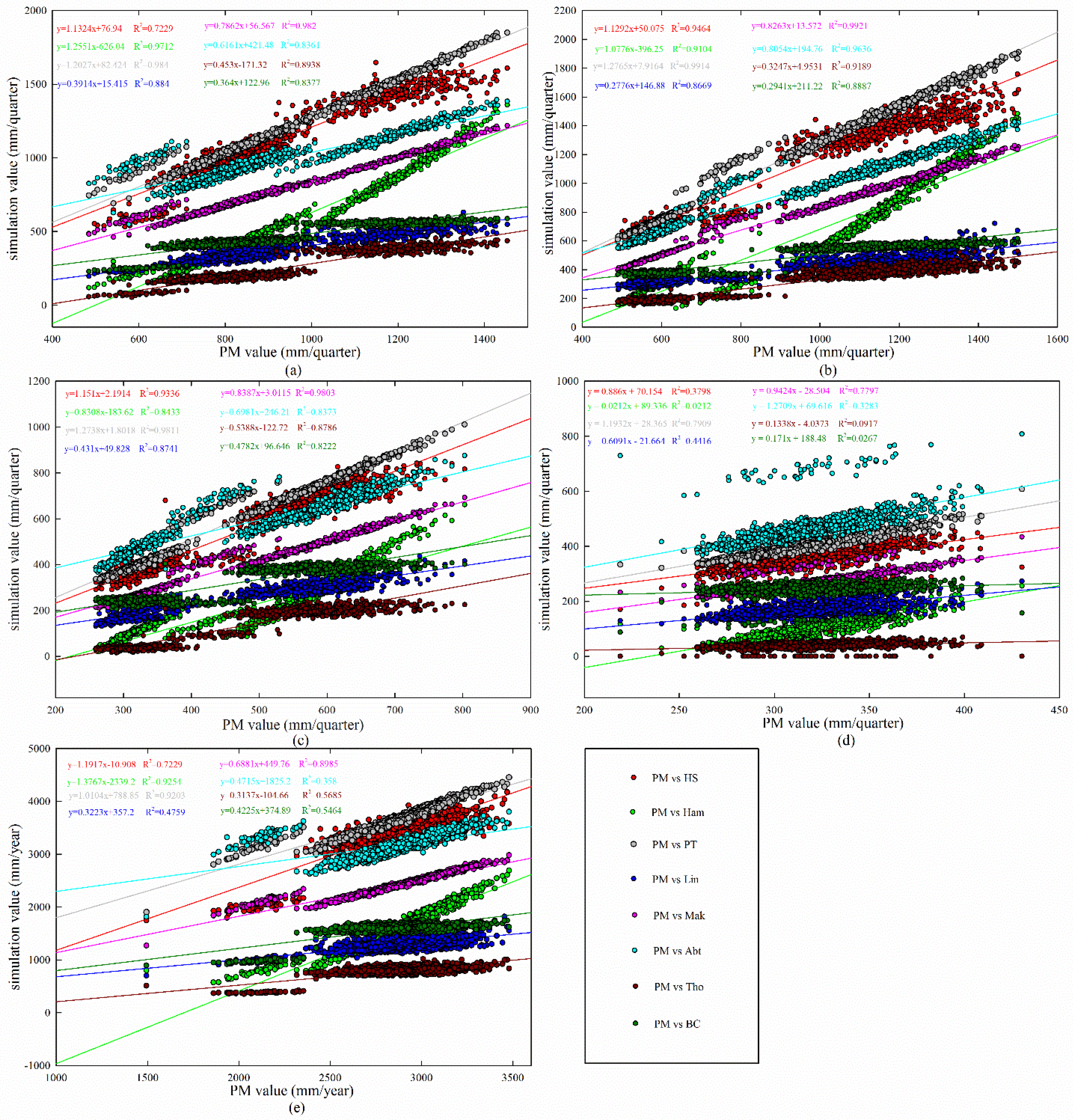
To understand the relationship between PM and the eight other methods, NSE, Re, and NRMSE values for one year and four seasons are listed in Table 3. Yearly, NSE values ranged from −58.724 to −1.040. Results for Abt and Mak were −1.040 and −1.857, respectively, while the others were much smaller than zero. Compared to Re, Abt, Mak and HS performed better with values 0.110, −0.155 and 0.188, respectively. With respect to the NRMSE values, Abt performed the best with the lowest value of 0.134. Considering the coefficient of determination (R2) of the linear regression between PM and the eight other methods (Figure 2e), Ham performed the best with the value of 0.925 followed by PT (0.920) and Mak (0.899). The results indicated that no methods performed well yearly, but Mak and Abt were narrowly acceptable.
The seasonal statistical analysis between the measured and simulated PET are shown in Table 3 and Figure 2. For spring, Abt performed the best with the highest value of NSE (0.664), the lowest value of |Re| (0.075), the lowest value of NRMSE (0.129), and a higher value of R2 (0.836). Mak was in the second place with NSE of 0.477, R2 of 0.982, |Re| of 0.152 and NRMSE of 0.161. Although the R2 value of PT was close to 1, the results of other statistical analysis showed poor performance. It indicated that PT is unacceptable for PET simulation for spring.
For summer, Abt performed the best with the highest value of NSE (0.937), the lowest values of |Re| (0.007), the lowest value of NRMSE (0.076,) and high value of R2 (0.964), as shown in Table 3 and Figure 2b. Mak performed the second best with the values of NSE = 0.691, |Re| = 0.160, NRMSE = 0.170, and R2 = 0.992.
For autumn, the applicability of each method was not similar to that for yearly, spring, and summer. Mak performed the best with the highest value of NSE (0.630), the lowest value of |Re| (0.155), the lowest value of NRMSE (0.164), and the second highest value of R2 (0.980) (Table 3 and Figure 2c). HS performed the second best with NSE = 0.552, |Re| = 0.155, NRMSE = 0.181, and R2 = 0.934. Although PT owned the highest R2 (0.981), other statistical analysis of PT appeared poor which indicated that PT performed not well in autumn.
For winter, Mak was the best estimation method with the highest value of NSE (0.886), the smallest value of |Re| (0.148), the smallest value of NRMSE (0.173), and the value of R2 = 0.7797, which indicated that this method was acceptable and available.

3.3. Yun-Gui Plateau

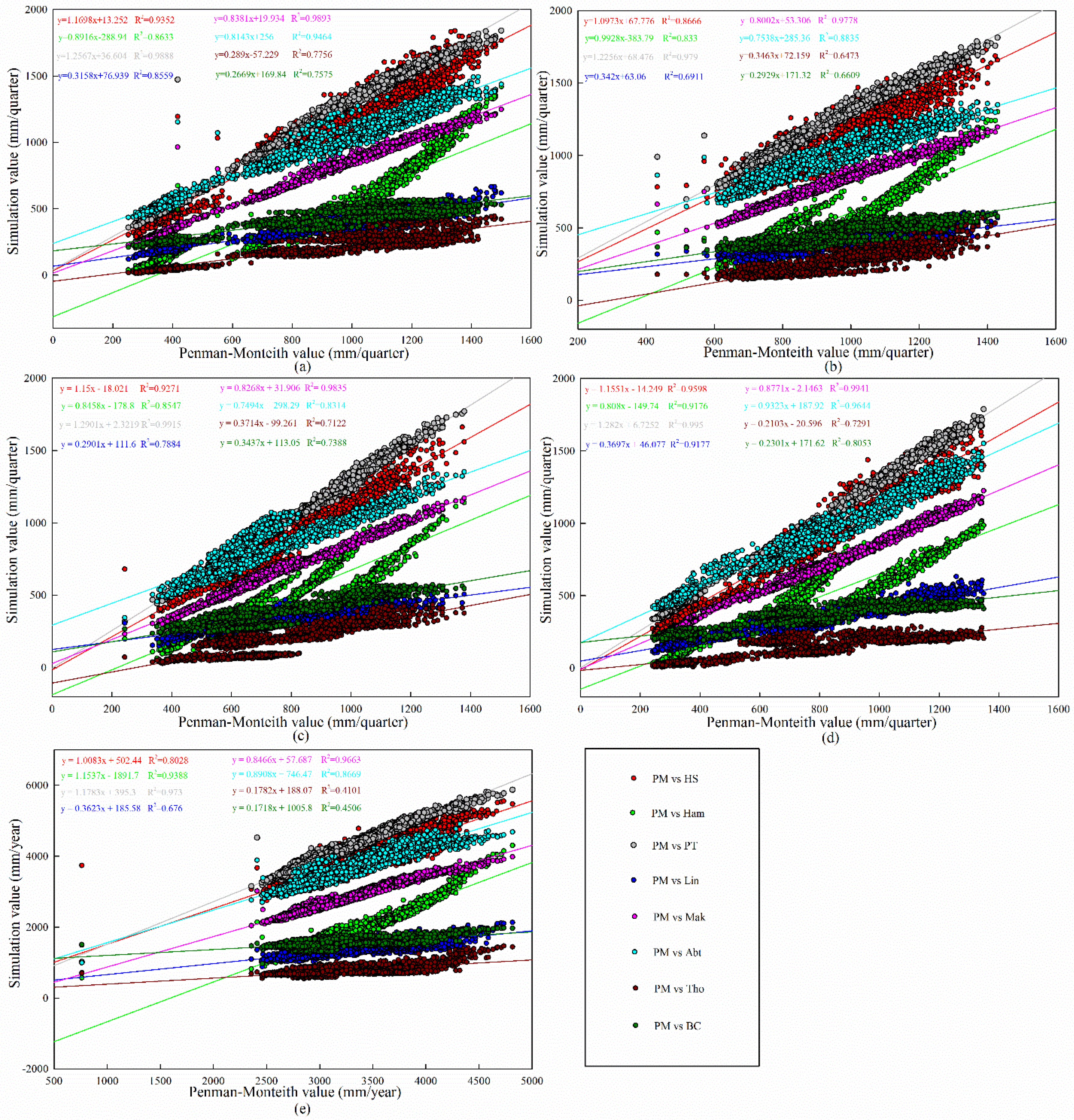
As seen in Table 3 and Figure 3e, for year, the NSE values of Abt and Mak were 0.334 and 0.138, respectively, and the Re and NRMSE values were 0.110 and −0.136, and 0.123 and 0.140, respectively. It indicated that these two methods estimated PET well. The values of R2 of PT, Mak, Ham, and Abt indicated that these methods were efficient (R2 > 0.850). The overall results showed that Abt was the best method to perform year PET in this region, followed by Mak.
For spring, the NSE values of Abt, HS and Mak were above 0.2, especially for Abt whose NSE was 0.845 (Table 4 and Figure 3a). The Re and NRMSE of Abt, Mak and HS were lower. The Re value ranged from −0.140 to 0.185, and the NRMSE was in the range 0.127–0.217. As for Mak, PT, Abt and HS, the R2 values were above 0.93, which indicated that these four methods performed well. These results showed that Abt was the best estimate method to simulate PET for the region in spring, followed by Mak and HS. Although PT owned the highest value of R2 (0.989), its other statistical parameter values were not useful, indicating that this estimation model is not acceptable and applicable.
For summer (Table 4 and Figure 3b), the NSE values were above 0.10 for Abt, Mak and HS. Abt showed the highest NSE value of 0.805. The Re values ranged from −0.145 to 0.168 for Abt, Mak and HS, while the NRMSE values were between 0.089 and 0.190. Note that the Re and NRMSE values of Abt were close to zero. The R2 value of PT was the highest (0.979) followed by Mak (0.978), both close to 1. Similar for year and spring, Abt displayed the best performance followed by Mak and HS.
As for autumn (Table 4 and Figure 3c), the NSE values of Mak, HS, and Abt were higher than 0.58. The Re and NRMSE values were low for Mak, HS and Abt. The values of Re ranged from −0.132 to 0.136, while the values of NRMSE ranged from 0.144 to 0.180. The values of R2 were higher than 0.830 for Mak, HS and Abt. These results indicated that Mak, HS and Abt were all acceptable and applicable, among which Mak was the best.
NSE values of four methods performed well among which the values of Mak and HS were 0.886 and 0.803, respectively. For these methods, the Re values ranged from −0.126 to 0.185, while NRMSE ranged from 0.138 to 0.201. The values of R2 were above 0.80 except for Tho method; the highest value of R2 was shown by PT. For winter, Mak was the best choice followed by HS and Abt.

3.4. The Eastern Margin of the Tibetan Plateau

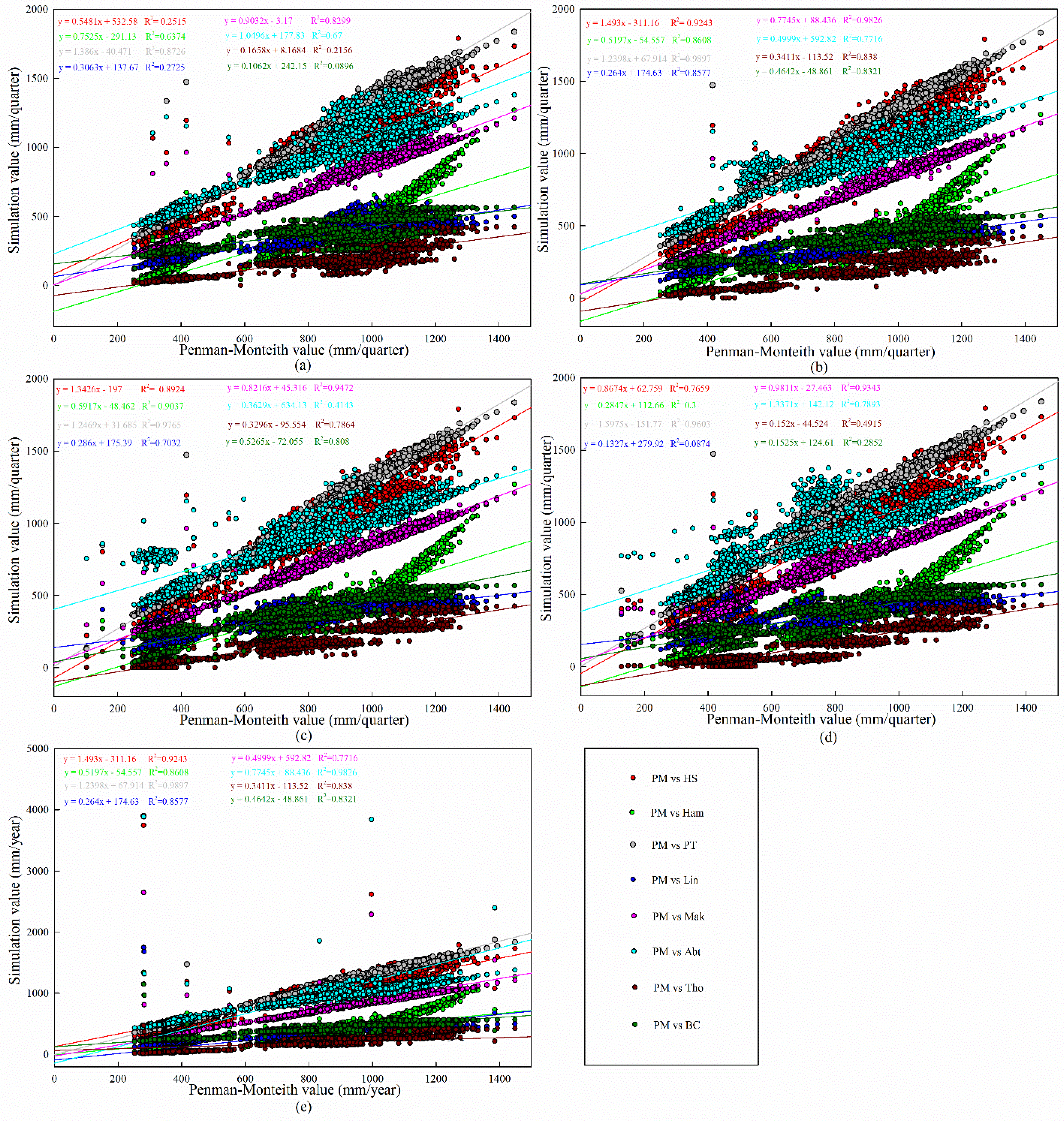
A comparative evaluation of error and regression analysis indicated that Mak performed the best for yearly scale with the highest NSE (0.238), the second lowest |Re| (0.095), the lowest NRMSE (0.120) and high R2 value of 0.983 (Table 5 and Figure 4e). The other methods were not quite suitable for yearly scale in this region.
The spring results were similar to those of yearly; only Mak was acceptable and applicable with the highest NSE (0.049), the lowest |Re| (0.100) and NRMSE (0.111), and the second-highest R2 (0.830) (Table 5 and Figure 4a). The NSE values were not good for spring and yearly scale because, not only was the value of Mak close to 0 (lying above 0), but the value of the seven other methods were also very low, lying below 0. The R2 values were also low; most of them were below 0.9.
The Mak and HS performed the best and second best, respectively, in summer and autumn (Table 5 and Figure 4b,c). In summer, Mak showed the highest NSE (0.747) and second-highest R2 (0.983), the lowest |Re| (0.123) and the lowest NRMSE (0.142). HS also could be used to estimate PET with the second-highest NSE (0.351), high R2 (0.924), the second-lowest |Re| (0.133) and the second-lowest NRMSE (0.227). In autumn, the NSE values of Mak and HS were above 0.6, which generated good simulation results, 0.849 and 0.665, respectively. The Re values of Mak and HS were closed to 0, especially HS whose Re value was −0.004. Mak had the lowest NRMSE (0.135), while HS owned the second-lowest value (0.201). Five methods had R2 values above 0.8, and PT owned the highest value of 0.977. These results showed that Mak was the best method to estimate PET followed by HS in summer and autumn.
In winter (Table 5 and Figure 4e), the NSE values of Mak and HS were 0.860 and 0.738, respectively, both of them close to 1. The Re values of Mak (−0.064) and HS (−0.029) were very close to zero. The NRMSE values of Mak and HS were 0.090 and 0.123, respectively. The highest R2 value was 0.960, which belonged to PT, while Mak showed the second-highest value of 0.934; however, HS showed a low R2 value (0.766), which was below 0.8. These results indicated that Mak was the best method to estimate PET in winter in this region.

3.5. Arid River Valley Region

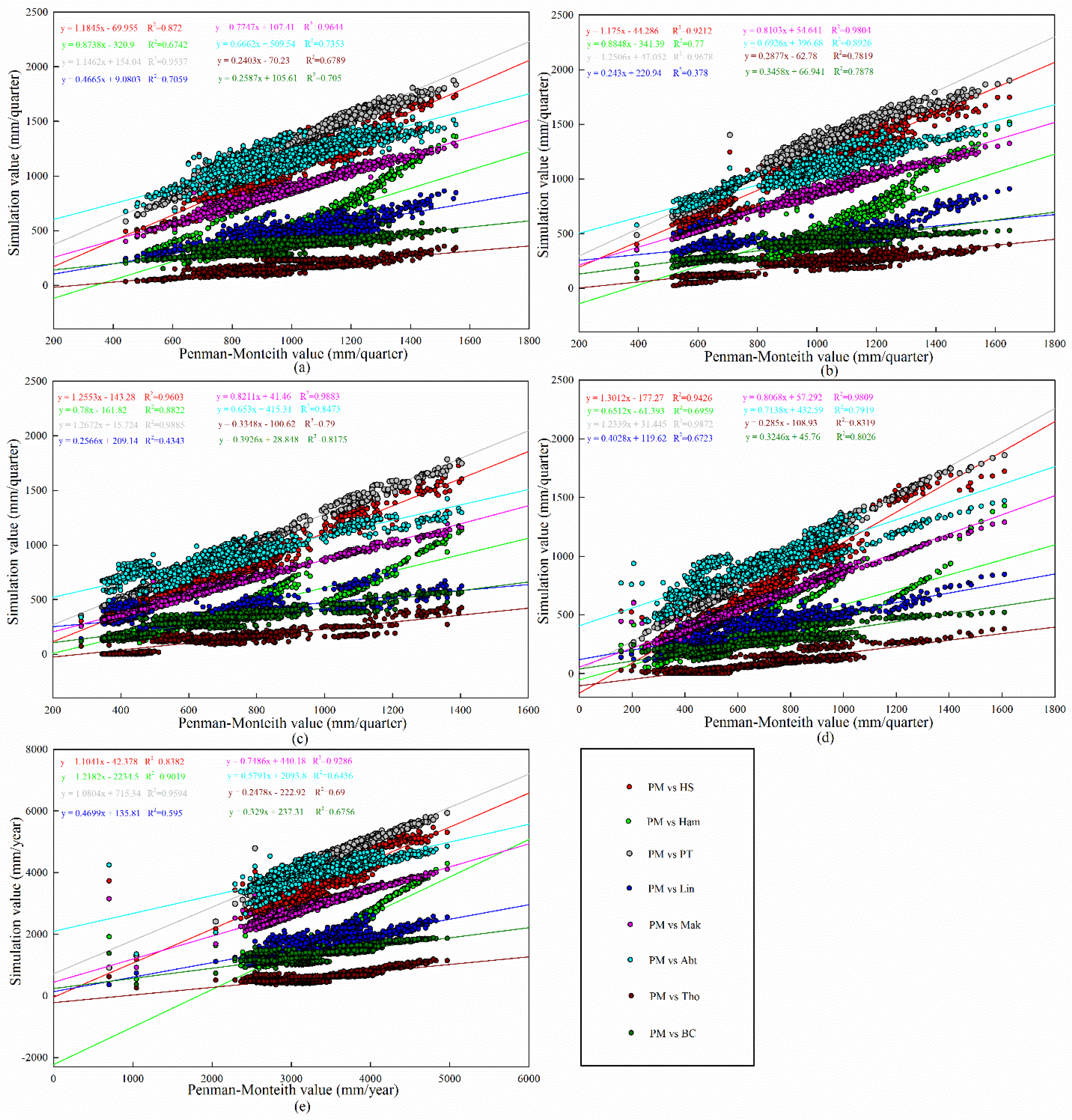
For yearly scale (Table 6 and Figure 5e), only NSE values of two methods were above 0, viz. HS (0.433) and Mak (0.344). The Re value of HS was close to zero, while for Mak, it was −0.120. As for NRMSE value, HS had the lowest value (0.121) and Mak owned the second-lowest (0.131). Four methods had R2 values above 0.8; PT had the highest value while HS had the lowest value among these four methods. These results indicated that HS was the best and Mak was the second-best for yearly scale in this region.
The spring simulation result was contrary to the yearly results (Table 6 and Figure 5a). Mak, with the highest NSE (0.600) and R2 (0.964), the lowest NRMSE (0.129) and the second-lowest |Re| (0.117), was the best performing method. The second was HS, which had the lowest |Re| (0.114), the second-highest NSE (0.449), the second-lowest NRMSE (0.152) and high R2 (0.872).
For summer (Table 6 and Figure 5b), the highest NSE and high R2 values was obtained for Abt, about 0.677 and 0.893, respectively, as well as the lowest |Re| and NRMSE, about 0.097 and 0.134, respectively, indicating that Abt performed the best. Mak was the second with the highest R2 values, about 0.980, the second-highest NSE (0.628), and low |Re| (0.134) and NRMSE (0.144). The third was HS with high NSE (0.548) and R2 (0.921), and low |Re| (0.130) and NRMSE (0.150).
For autumn (Table 6 and Figure 5c), the NSE values of HS and Mak were above 0.8, and the Re values for these two methods were 0.055 and −0.120 for HS and Mak, respectively. The NRMSE values of these two methods were quite close: 0.132 and 0.140, respectively. Although the R2 value of PT was the highest, its simulation result to estimate PET was not acceptable and applicable due to its poor values in the three other statistical parameters.
For winter (Table 6 and Figure 5d), Mak was the best simulation method with the highest NSE (0.861), the lowest NRMSE (0.132), the second-lowest |Re| (0.107), and high R2 (0.981). HS was in the second place with the second highest NSE (0.797), high R2 (0.988), the lowest |Re| (0.120), and second lowest NRMSE (0.140).

4. Discussion

This paper compared eight different methods for the evaluation of PET with PM in southwestern China. We applied three radiation-based methods (PT, Mak, and Abt) and five temperature-based methods (Tho, Ham, Lin, HS, and BC), all of which showed large differences in their applicability. The radiation-based methods showed better performance than the temperature-based methods in the evaluation of PET in the study area. This is in accordance with findings of previous studies in other regions [25,49,50].
Among the radiation-based methods, Mak showed the best performance followed by the Abt and PT. These three methods were established in a humid climate condition, which are suitable for regions with abundant rainfall like our study area. This is probably one of the reasons they can be used to estimate PET in the study area. Mak showed less errors and high correlation comparable with PM among the radiation-based methods used in the present study. Lu et al. [11] suggested Mak with poor performance in the southeastern United States, whereas Tukimat et al. [49] reported that Mak performed the best among the studied methods in Malaysia. The reason for these different results may be that the same method yielded different results under different climatic conditions and geographical environments. PT was acceptable and applicable to evaluate PET during the winter in Yun-Gui plateau because of its third place among the three methods which can evaluate PET in this situation. Wei and Menzel [51] believed PT to be the most suitable method for global application in the estimation of PET. However, Abt only needs two parameters to estimate ET compared to PT which requires five parameters. Therefore, Abt can be used more easily than PT in estimating PET in the study area.
Among the temperature-based methods, only HS can be used to estimate PET, but it was not the best simulation method in the study area. HS can be used on all time scales in arid river valley region, possibly because it was established in an arid and semi-arid climate condition, and the present study area has a similar climate condition to some extent, i.e., the arid river valley region. Meanwhile, the input parameters of the HS included extraterrestrial solar radiation while other temperature-based methods exclude this, which might be the reason that only HS can be used to estimate PET in the study region. Chen et al. [13], Lu et al. [11] and Nikam et al. [52] found that Tho performed worse in many regions. In the present study, Tho also showed the worst performance among all the selected methods. This is probably because Tho is only based on temperature, i.e. only single input parameter. Another reason might be that Tho was established in a humid climate and the underlying surface was a valley, and PET is determined by other variables such as humidity, wind speed, vapor pressure and solar radiation. However, Tho was found to be a suitable method for PET estimation in Malaysia [48,53]. Besides, other temperature-based methods were also found to be unsatisfactory in PET estimation in the study area due to the high error analysis and poor correlation.
The four statistical indicators showed various simulation effects. On a seasonal scale, NSE showed simulation methods match FAO-PM method better than annual except for the eastern margin of the Tibetan Plateau. The greatest disadvantage of NSE was that calculations of squared values were required to show the relationships between the measured and the simulated values. As a result, larger values were strongly overestimated while the lower values were neglected [54,55]. The three other indicators presented no special features in annual and seasonal scales. Overall, the simulation effects of the four statistical indicators in the eastern margin of the Tibetan Plateau were poorer than the other three regions. The high altitude, changeable weather and complex terrain may be responsible for such results. PBIAS suggested that Abt, PT, and HS overestimate PET, while the other five models typically underestimate PET.
All the selected methods comparable with PM showed different simulation results, in which some methods viz. Mak and Abt led to good estimation, some viz. PT and HS were acceptable and applicable, while some viz. Ham, Lin, Tho and BC were completely unusable to estimate PET. The input parameters may be the main factors that affected their performance. Different methods need different input parameters. Another important reason is that each method was established on a specific underlying surface and climate conditions; however, the study area has complex topography and changeable weather. The heterogeneity problem in the climate data we used may be influenced by climate or non-climate factors [56,57] (including the relocation of weather stations and observation methods, urbanization, and agricultural irrigation).

5. Conclusions

From the above analysis, it can be concluded that the radiation-based methods were more suitable for estimating PET in southwest China. Among the radiation-based methods, Mak performed the best, Abt was second, and PT was third. Among the temperature-based methods, HS was the only one which was acceptable and applicable, while the others showed a poor performance in evaluating PET, especially Tho. Besides, the PET values of HS, PT, and Abt were lager than PM, while Ham, Lin, Mak, Tho, and BC were smaller than PM.
For Sichuan basin, Mak performed the best for year, autumn and winter PET estimations, while Abt was the most suitable for spring and summer. For the Yun-Gui plateau, Abt was perfect for estimating in year, spring and summer PET, while, Mak performed the best for autumn and winter. In the eastern margin of the Tibetan Plateau, Mak was the most suitable for all time scales. On the other hand, for the arid river valley region, HS ranked first in year and autumn PET estimations, Mak performed the best for spring and winter, and Abt was perfect for summer.
To some extent, it is expected that the conclusions of this study can be used in regions with similar topography and climatic conditions in the world. If a region is featured with low latitude, warm and moist climate similar to Sichuan basin, or if a region is a plateau having monsoon climate with low latitude, Mak and Abt can be used to estimate PET. Researchers may be able to use Mak in regions that are similar to the eastern margin of the Tibetan Plateau. If a region has abundant rainfall but high evaporation, and intensive solar radiation similar to the arid river valley region in this study, Mak and HS may be suitable for PET estimating. A region whose geographic feature is complex and climate varies greatly similar to southwest China, Mak can be recommended. We hope that the present study will be helpful in general to select the appropriate methods according to the availability of meteorological data.

Acknowledgments

This work is jointly supported by the National Natural Science Foundation of China (41601028), and China Postdoctoral Science Foundation funded project (2012M511938).

Author Contributions

Jiangkun Zheng was responsible for the original idea of the study; Jiaqi Shi and Feng Liao were responsible for the data compilation; Xing Ma, Wenwu Wang and Xuli Chen were responsible for data processing and drawing; Mingfang Zhang was responsible for revising the article; and Dengxiao Lang drafted the manuscript and all authors read and revised the final manuscript.

Conflicts of Interest

The authors declare no conflict of interest.

References

  1. Almorox, J.Y.; Hontoria, C. Global solar radiation estimation using sunshine duration in Spain. Energy Convers. Manag. 2004, 45, 1529–1535. [Google Scholar] [CrossRef]
  2. Khoob, A.R. Comparative study of Hargreaves’s and artificial neural network’s methodologies in estimating reference evapotranspiration in a semiarid environment. Irrig. Sci. 2008, 26, 253–259. [Google Scholar] [CrossRef]
  3. Singh, R.K.; Pawar, P.S. Comparative study of reference crop evapotranspiration (ETO) by different energy based method with FAO 56 Penman-Monteith method at New Delhi, India. Eng. Sci. Technol. 2011, 3, 7861–7868. [Google Scholar]
  4. Amatya, D.M.; Harrison, C.A.; Trettin, C.C. Comparison of potential evapotranspiration (PET) using three methods for a grass reference and a natural forest in Coastal Plain of South Carolina. Proceeding of the 2014 South Carolina Water Resources Conference, Columbia, SC, USA, 14–16 October 2014; Available online: http://tigerprints.clemson.edu/cgi/viewcontent.cgi?article=1298&context=scwrc (accessed on 25 September 2017).
  5. Bandyopadhyay, A.; Bhadra, A.; Swarnakar, R.K.; Raghuwanshi, N.S.; Singh, R. Estimation of reference evapotranspiration using a user-friendly decision support system: DSS_ET. Agric. For. Meteorol. 2012, 154–155, 19–29. [Google Scholar] [CrossRef]
  6. Ding, R.; Kang, S.; Li, F.; Zhang, Y.; Tong, L. Evapotranspiration measurement and estimation using modified Priestley–Taylor model in an irrigated maize field with mulching. Agric. For. Meteorol. 2013, 168, 140–148. [Google Scholar] [CrossRef]
  7. Allen, R.G.; Masahiro, T.; Ricardo, T. Satellite-based energy balance for mapping evapotranspiration with internalized calibration (METRIC)—Model. J. Irrig. Drain. Eng. 2007, 133, 380–394. [Google Scholar] [CrossRef]
  8. Senay, G.B.; Budde, M.; Verdin, J.P.; Melesse, A.M. A coupled remote sensing and simplified surface energy balance approach to estimate actual evapotranspiration from irrigated fields. Sensors 2007, 7, 979–1000. [Google Scholar] [CrossRef]
  9. Wagle, P.; Bhattarai, N.; Gowda, P.H.; Kakani, V.G. Performance of five surface energy balance models for estimating daily evapotranspiration in high biomass sorghum. ISPRS J. Photogramm. Remote Sens. 2017, 128, 192–203. [Google Scholar] [CrossRef]
  10. Allen, R.G.; Pereira, L.S.; Raes, D.; Smith, M. Crop Evapotranspiration: Guidelinse for Computing Crop Water Requirements. Fao Irrigation and Drainage Paper 56; FAO-Food and Agriculture Organization of the United Nations Rome: Rome, Italy, 1998. [Google Scholar]
  11. Lu, J.; Sun, G.; Mcnulty, S.G.; Amatya, D.M. A comparison of six potential evapotranspiration methods for regional use in the Southeastern United States. J. Am. Water Resour. Assoc. 2005, 41, 621–633. [Google Scholar] [CrossRef]
  12. Liu, X.; Lin, E. Performance of the Priestley–Taylor equation in the semiarid climate of North China. Agric. Water Manag. 2005, 71, 1–17. [Google Scholar]
  13. Chen, D.; Gao, G.; Xu, C.; Guo, J.; Ren, G. Comparison of the Thornthwaite method and pan data with the standard Penman–Monteith estimates of reference evapotranspiration in China. Clim. Res. 2005, 28, 123–132. [Google Scholar] [CrossRef]
  14. Berti, A.; Tardivo, G.; Chiaudani, A.; Rech, F.; Borin, M. Assessing reference evapotranspiration by the Hargreaves method in north-eastern Italy. Agric. Water Manag. 2014, 140, 20–25. [Google Scholar] [CrossRef]
  15. Oudin, L.; Hervieu, F.; Michel, C.; Perrin, C.; Andréassian, V.; Anctil, F.; Loumagne, C. Which potential evapotranspiration input for a lumped rainfall–runoff model?: Part 2—Towards a simple and efficient potential evapotranspiration model for rainfall–runoff modelling. J. Hydrol. 2005, 303, 290–306. [Google Scholar] [CrossRef]
  16. Tegos, A.; Malamos, N.; Koutsoyiannis, D. A parsimonious regional parametric evapotranspiration model based on a simplification of the Penman–Monteith formula. J. Hydrol. 2015, 524, 708–717. [Google Scholar] [CrossRef]
  17. McMahon, T.A.; Finlayson, B.L.; Peel, M.C. Historical developments of models for estimating evaporation using standard meteorological data. Wiley Interdiscip. Rev. Water 2016, 3, 788–818. [Google Scholar] [CrossRef]
  18. Allen, R.G.; Clemmens, A.J.; Burt, C.M.; Solomon, K.; O’Halloran, T. Prediction accuracy for projectwide evapotranspiration using crop coefficients and reference evapotranspiration. J. Irrig. Drain. Eng. 2005, 131, 24–36. [Google Scholar] [CrossRef]
  19. Allen, R.G.; Pruitt, W.O.; Wright, J.L.; Howell, T.A.; Ventura, F.; Snyder, R.; et al. A recommendation on standardized surface resistance for hourly calculation of reference ETO by the FAO 56 Penman-Monteith method. Agric. Water Manag. 2006, 81, 1–22. [Google Scholar] [CrossRef]
  20. Gong, L.; Xu, C.Y.; Chen, D.; Halldin, S.; Chen, Y.D. Sensitivity of the Penman–Monteith reference evapotranspiration to key climatic variables in the Changjiang (Yangtze River) basin. J. Hydrol. 2006, 329, 620–629. [Google Scholar] [CrossRef]
  21. Al-Ghobari, H.M. Estimation of reference evapotranspiration for southern region of Saudi Arabia. Irri Sci. 2000, 19, 81–86. [Google Scholar] [CrossRef]
  22. De Bruin, H.A.R.; Stricker, J.N.M. Evaporation of grass under non-restricted soil moisture conditions. Hydrol. Sci. J. 2000, 45, 391–406. [Google Scholar] [CrossRef]
  23. Jacobs, J.M.; Satti, S.R. Evaluation of Reference Evapotranspiration Methodologies and Afsirs Crop Water Use Simulation Model: Final Report; University of Florida: Gainesville, FL, USA, 2001. [Google Scholar]
  24. Garcia, M.; Raes, D.; Allen, R.; Herbas, C. Dynamics of reference evapotranspiration in the Bolivian highlands (Altiplano). Agric. For. Meteorol. 2004, 125, 67–82. [Google Scholar] [CrossRef]
  25. Xu, C.; Chen, D. Comparison of seven models for estimation of evapotranspiration and groundwater recharge using lysimeter measurement data in Germany. Hydrol Process. 2005, 19, 3717–3734. [Google Scholar] [CrossRef]
  26. Xu, C.; Gong, L.; Jiang, T.; Chen, D.; Singh, V.P. Analysis of spatial distribution and temporal trend of reference evapotranspiration and pan evaporation in Changjiang (Yangtze River) catchment. J. Hydrol. 2006, 327, 81–93. [Google Scholar] [CrossRef]
  27. Raziei, T.; Pereira, L.S. Estimation of ETo with Hargreaves–Samani and FAO-PM temperature methods for a wide range of climates in Iran. Agric. Water Manag. 2013, 121, 1–18. [Google Scholar] [CrossRef]
  28. Thornthwaite, C.W. An approach toward a rational classification of climate. Geogr. Rev. 1948, 38, 55–89. [Google Scholar] [CrossRef]
  29. Abtew, W. Evapotranspiration measurements and modeling for three wetland systems in south Florida. J. Am. Water Resour. Assoc. 1996, 32, 465–473. [Google Scholar] [CrossRef]
  30. Hargreaves, G.H.; Samani, Z.A. Reference crop evapotranspiration from temperature. Appl. Eng. Agric. 1985, 1, 96–99. [Google Scholar] [CrossRef]
  31. Brouwer, C.; Heibloem, M. Irrigation Water Management: Irrigation Water Needs: Training Manual No.3; FAO Land and Water Development Division: Rome, Italy, 1986. [Google Scholar]
  32. Hamon, W.R. Computation of direct runoff amounts from storm rainfall. Int. Assoc. Sci. Hydrol. Pub. 1963, 63, 52–62. [Google Scholar]
  33. Linacre, E.T. A simple formula for estimating evaporation rates in various climates, using temperature data alone. J. Agric. Meteorol. 1977, 18, 409–424. [Google Scholar] [CrossRef]
  34. Priestley, C.H.B.; Taylor, R.J. On the assessment of surface heat flux and evaporation using large-scale parameters. Mon. Weather Rev. 1972, 100, 81–92. [Google Scholar] [CrossRef]
  35. Makkink, G.F. Testing the Penman formula by means of lysimeters. J. Inst. Water Eng. 1957, 11, 277–288. [Google Scholar]
  36. Li, Y.; Xu, H.; Liu, D. Features of the extremely severe drought in the east of southwest China and anomalies of atmospheric circulation in summer 2006. Acta Meteorol. Sin. 2011, 25, 176–187. [Google Scholar] [CrossRef]
  37. Zhang, W.; Jin, F.; Zhao, J.; Qi, L.; Ren, H. The possible influence of a nonconventional El Niño on the severe autumn drought of 2009 in Southwest China. J. Clim. 2013, 26, 8392–8405. [Google Scholar] [CrossRef]
  38. Zhang, L.; Xiao, J.; Li, J.; Wang, K.; Lei, L.; Guo, H. The 2010 spring drought reduced primary productivity in southwestern China. Environ. Res. lett. 2012, 7, 045706. [Google Scholar] [CrossRef]
  39. Lv, L. Geography of China; Science Press: Beijing, China, 2012; Available online: http://202.115.182.3:8080/opac/book/a2c2df0859a38b1e0b5544ac7a617e8a (accessed on 22 September 2017). (In Chinese)
  40. Zhao, J.; Chen, C. Geography of China; Higher Education Press: Beijing, China, 1999; Available online: http://book.ixueshu.com/book/3d20d9eb5a0768e2.html (accessed on 22 September 2017). (In Chinese)
  41. Kottek, M.; Grieser, J.; Beck, C.; Rudolf, B.; Rubel, F. World Map of the Köppen-Geiger climate classification updated. Meteorol. Z. 2006, 15, 259–263. [Google Scholar] [CrossRef]
  42. National Science & Technology Infrastructure. Available online: http://data.cma.cn/ (accessed on 8 May 2014). (In Chinese).
  43. Li, Z.; He, Y.; An, W.; Song, L.; Zhang, W.; Catto, N.; Wang, Y.; Wang, S.; Liu, H.; Cao, W.; Theakstone, W.H.; Wang, S.; Du, J. Climate and glacier change in southwestern China during the past several decades. Environ. Res. Lett. 2011, 6, 045404. [Google Scholar] [CrossRef]
  44. Pang, X.; Bao, W.; Wu, N. Reasons of dry valley climate characteristic and its formation reason in upstream of Mingjiang river. Resour. Environ. Yangtze Basin 2008, 17, 48–55. [Google Scholar]
  45. China Meteorological Administration. Classification of Meteorological Drought; China Meteorological Press: Beijing, China, 2006. [Google Scholar]
  46. Nash, J.E.; Sutcliffe, J.V. River flow forecasting through conceptual models part Ι–A discussion of principles. J. Hydrol. 1970, 10, 282–290. [Google Scholar] [CrossRef]
  47. Daut, I.; Irwanto, M.; Irwan, Y.M.; Gomesh, N.; Ahmad, N.S. Combination of Hargreaves method and linear regression as a new method to estimate solar radiation in Perlis, Northern Malaysia. Sol. Energy 2011, 85, 2871–2880. [Google Scholar] [CrossRef]
  48. Gupta, H.V.; Sorooshian, S.; Yapo, P.O. Status of automatic calibration for hydrologic models: Comparison with multilevel expert calibration. J. Hydrol. Eng. 1999, 4, 135–143. [Google Scholar] [CrossRef]
  49. Tukimat, N.N.A.; Harun, S.; Shahid, S. Comparison of different methods in estimating potential evapotranspiration at Muda Irrigation Scheme of Malaysia. J. Agric. Rural Dev. Trop. Subtrop. 2012, 113, 77–85. [Google Scholar]
  50. Jadhav, P.B.; Kadam, S.A.; Gorantiwar, S.D. Comparison of methods for estimating reference evapotranspiration (ETO) for Rahuri region. J. Agrometeorol. 2015, 17, 204–207. [Google Scholar]
  51. Wei, M.; Menzel, L. A global comparison of four potential evapotranspiration equations and their relevance to stream flow modeling in semi-arid environments. Adv. Geosci. 2008, 18, 15–23. [Google Scholar]
  52. Nikam, B.; Kumar, P.; Garg, V.; Thakur, P.K.; Aggarwal, S.P. Comparative evaluation of different potential evapotranspiration estimation approaches. Int. J. Res. Eng. Technol. 2014, 3, 544–552. [Google Scholar]
  53. Mohd, E.T.; Mazlin, M.; Muhamad, B.G.; Sharifah, M.S.A.; Osman, J.; Nor, A.A.A. Water resources study and modeling at north Kedah: A case of Kubang Pasu and Padang Terap water supply schemes. Res. J. Earth Sci. 2009, 1, 35–42. [Google Scholar]
  54. Legates, D.R.; McCabe, G.J. Evaluating the use of “goodness-of-fit” measures in hydrologic and hydroclimatic model validation. Water Resour. Res. 1999, 35, 233–241. [Google Scholar] [CrossRef]
  55. Krause, P.; Boyle, D.P.; Base, F.B. Comparison of different efficiency criteria for hydrological model assessment. Adv. Geosci. 2005, 5, 89–97. [Google Scholar] [CrossRef]
  56. Sahi̇n, S.; Ci̇gi̇zoglu, H.K. Homogeneity analysis of Turkish meteorological data set. Hydrol. Process. 2010, 24, 981–992. [Google Scholar] [CrossRef]
  57. Chu, R.; Li, M.; Shen, S.; Islam, A.R.M.T.; Cao, W.; Tao, S.; Gao, P. Changes in reference evapotranspiration and its contributing factors in Jiangsu, a major economic and agricultural province of eastern China. Water 2017, 9, 486. [Google Scholar] [CrossRef]
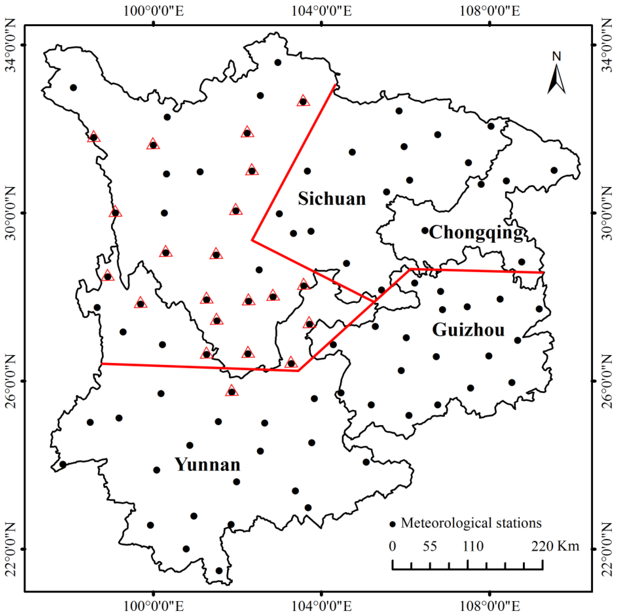
Figure 1. Location of the weather stations in southwestern China. (The red lines were dividing lines which divided the study region into three zones; and Δ in red represents the weather stations in arid river valley region which belongs to one of the three parts.)
Water 09 00734 g001
Figure 2. Linear regression of measured and simulation values in Sichuan basin: (a) spring; (b) summer; (c) autumn; (d) winter; and (e) annual.
Water 09 00734 g002
Figure 3. Linear regression of measured and simulation values in the Yun-Gui plateau: (a) spring; (b) summer; (c) autumn; (d) winter; and (e) annual.
Water 09 00734 g003
Figure 4. Linear regression of measured and simulation values in the eastern margin of the Tibetan Plateau: (a) spring; (b) summer; (c) autumn; (d) winter; and (e) annual.
Water 09 00734 g004
Figure 5. Linear regression of measured and simulation values in the arid river valley region: (a) spring; (b) summer; (c) autumn; (d) winter; and (e) annual.
Water 09 00734 g005
Table 1. Annual and seasonal PET estimated by FAO–PM method in the four sub-regions.
RegionsPET (mm)
AnnualSpringSummerAutumnWinter
Sichuan basin2860.2917.6967.4495.9479.3
Yun-Gui plateau3374.6926.3947.7754.8745.8
The eastern margin of the Tibetan Plateau2993.4956.1864.4569.0603.9
Arid river valley region3347.5991.7978.0711.5664.2
Table 2. Annual and seasonal PBIAS (%) in the four sub-regions a.
RegionsTime HSHamPTLinMakAbtThoBC
SCBAnnual−18.79 44.12 −28.62 55.28 15.46 −10.97 72.29 44.64
Spring−21.63 42.72 −29.26 59.18 15.22 −7.55 73.37 50.20
Summer−18.09 33.20 −28.46 57.05 15.97 −0.68 67.02 48.76
Autumn−15.54 53.94 −27.74 46.85 15.52 −19.46 70.87 32.70
Winter−18.11 58.70 −28.62 52.94 14.84 −29.54 82.33 38.05
YGPAnnual−15.62 40.28 −29.46 58.31 13.64 −11.04 76.65 53.22
Spring−18.48 42.28 −29.66 60.03 14.02 −9.28 77.31 54.81
Summer−16.75 40.47 −29.65 59.27 14.46 −49.41 72.84 52.97
Autumn−12.66 38.60 −29.31 56.52 13.19 −13.61 75.73 50.97
Winter−13.67 39.31 −29.10 56.81 12.58 −18.46 81.72 53.93
ETPAnnual−7.16 53.11 −33.14 48.62 9.46 −34.21 83.61 61.64
Spring−10.51 55.20 −34.37 54.97 10.01 −23.56 82.56 64.06
Summer−13.30 54.34 −31.86 53.40 12.32 −18.57 79.02 59.24
Autumn0.37 49.35 −30.26 40.57 9.88 −47.73 83.83 60.01
Winter2.87 52.88 −34.62 40.38 6.44 −57.24 92.18 64.12
ARVAnnual−9.14 45.09 −29.46 48.95 11.96 −20.60 81.90 59.99
Spring−11.40 44.97 −30.16 52.44 11.70 −18.00 83.05 63.48
Summer−12.98 46.35 −29.86 53.16 13.39 −9.74 77.64 58.59
Autumn−5.50 44.66 −29.07 44.90 11.96 −23.80 80.64 56.63
Winter−3.44 44.13 −28.12 41.71 10.70 −36.50 87.90 60.65
a: SCB means Sichuan basin; YGP means Yun-Gui plateau; ETP means the eastern margin of the Tibetan Plateau; ARV means arid river valley region
Table 3. Accuracy assessment of PET estimation in Sichuan basin.
Time ScalesEquationsHSHamPTLinMakAbtThoBC
YearNSE−3.578−21.338−8.363−34.177−1.857−1.040−58.724−22.051
Re0.188−0.4410.286−0.553−0.1550.110−0.723−0.446
NRMSE0.2010.4440.2880.5570.1590.1340.7260.451
SpringNSE−0.068−2.786−0.788−0.6440.4770.664−10.163−4.505
Re0.216−0.4270.293−0.592−0.1520.075−0.734−0.502
NRMSE0.2300.4340.2980.6080.1610.1290.7450.523
SummerNSE0.560−0.3040.039−3.0300.6910.937−4.290−2.063
Re0.181−0.3320.285−0.571−0.1600.007−0.670−0.488
NRMSE0.2020.3480.2990.6130.1700.0760.7020.534
AutumnNSE0.552−3.148−0.162−2.3610.6300.295−6.142−0.788
Re0.155−0.5390.277−0.469-0.1550.195−0.709−0.327
NRMSE0.1810.5500.2910.4950.1640.2270.7220.361
WinterNSE0.276−0.4500.617−0.4700.8860.611−2.097−0.016
Re0.181−0.5870.286−0.529−0.1480.295−0.823−0.381
NRMSE0.2700.6180.3180.6230.1730.3200.9040.518
Table 4. Accuracy assessment of PET estimation in the Yun-Gui plateau.
Time ScalesEquationsHSHamPTLinMakAbtThoBC
AnnualNSE−0.316−6.200−2.861−14.3260.1380.334−25.391−12.099
Re0.156−0.4030.295−0.583−0.1360.110−0.766−0.532
NRMSE0.1740.4060.2970.5920.1400.1230.7770.548
SpringNSE0.544−0.8610.068−2.9620.2230.845−5.295−2.459
Re0.185−0.4230.297−0.600−0.1400.093−0.773−0.548
NRMSE0.2170.4390.3110.6410.1520.1270.8080.599
SummerNSE0.116−3.219−1.242−8.1080.4320.805−12.520−6.432
Re0.168−0.4050.168−0.4050.168−0.4050.168−0.405
NRMSE0.1900.4150.3020.6090.1520.0890.7420.550
AutumnNSE0.667−1.061−0.203−3.6330.7350.585−6.824−2.813
Re0.127−0.3860.293−0.565−0.1320.136−0.757−0.510
NRMSE0.1610.4000.3060.6000.1440.1800.7800.545
WinterNSE0.803−0.0120.410−1.3270.8860.761−3.604−1.333
Re0.137−0.3930.291−0.568−0.1260.185−0.817−0.539
NRMSE0.1820.4130.3150.6260.1380.2010.8800.627
Table 5. Accuracy assessment of PET estimation in the eastern margin of the Tibetan Plateau.
Time ScalesEquationsHSHamPTLinMakAbtThoBC
AnnualNSE−0.454−14.142−4.988−12.0640.238−6.409−36.528−19.630
RE0.072−0.5310.331−0.846−0.0950.342−0.836−0.616
NRMSE0.1660.5360.3370.4980.1200.3750.8440.626
SpringNSE−0.952−22.931−8.559−23.0890.049−3.836−52.481−31.627
RE0.105 −0.552 0.344 −0.550 −0.100 0.236 −0.826 −0.641
NRMSE0.159 0.556 0.352 0.558 0.111 0.250 0.832 0.650
SummerNSE0.351 −3.006 −0.356 −3.156 0.747 0.240 −7.347 −3.764
RE0.133 −0.543 0.319 −0.534 −0.123 0.186 −0.790 −0.592
NRMSE0.227 0.563 0.328 0.574 0.142 0.245 0.813 0.614
AutumnNSE0.665 −1.228 0.141 −0.912 0.849 −1.485 −5.319 −2.283
RE−0.004 −0.493 0.303 −0.406 −0.099 0.477 −0.838 −0.600
NRMSE0.201 0.518 0.322 0.480 0.135 0.547 0.872 0.629
WinterNSE0.738 −4.575 −1.552 −2.779 0.860 −5.303 −14.556 −6.944
RE−0.029−0.5290.346−0.404−0.0640.572−0.922−0.641
NRMSE0.1230.5650.3830.4660.0900.6010.9450.675
Table 6. Accuracy assessment of PET estimation in the arid river valley region.
Time ScalesEquationsHSHamPTLinMakAbtThoBC
AnnualNSE0.433−7.018−2.389−8.6340.344−0.992−25.358−13.328
RE0.091−0.4510.295−0.489−0.1200.206−0.819−0.600
NRMSE0.1210.4570.2970.5010.1310.2280.8280.611
SpringNSE0.449−4.225−1.261−5.9550.600−0.046−6.109−9.221
RE0.114−0.4500.302−0.524−0.1170.180−0.831−0.635
NRMSE0.1520.4670.3070.5390.1290.2090.8460.654
SummerNSE0.548−3.116−0.721−4.7580.6280.677−10.384−5.641
RE0.130−0.4640.299−0.532−0.1340.097−0.776−0.586
NRMSE0.1580.4780.3090.5650.1440.1340.7950.607
AutumnNSE0.829−1.0920.072−1.6100.8080.241−5.829−2.542
RE0.055−0.4470.291−0.449−0.1200.238−0.806−0.566
NRMSE0.1320.4620.3080.5170.1400.2790.8350.602
WinterNSE0.797−0.8220.310−0.7900.861−0.253−5.541−2.346
RE0.034−0.4410.281−0.417−0.1070.365−0.879−0.607
NRMSE0.1620.4840.2980.4800.1340.4010.9170.656