Article

Quantification of Hydrological Responses Due to Climate Change and Human Activities over Various Time Scales in South Korea

1
Department of Civil Engineering, Pukyoung National University, Busan 48513, Korea
2
Department of Civil Engineering, Kangwon National University, Chuncheon 24341, Korea
*
Author to whom correspondence should be addressed.
Water 2017, 9(1), 34; https://doi.org/10.3390/w9010034
Submission received: 26 November 2016 / Revised: 30 December 2016 / Accepted: 4 January 2017 / Published: 8 January 2017

Abstract

:
Hydrological responses are being impacted by both climate change and human activities. In particular, climate change and regional human activities have accelerated significantly during the last three decades in South Korea. The variation in runoff due to the two types of factors should be quantitatively investigated to aid effective water resources’ planning and management. In water resources’ planning, analysis using various time scales is useful where rainfall is unevenly distributed. However, few studies analyzed the impacts of these two factors over different time scales. In this study, hydrologic model-based approach and hydrologic sensitivity were used to separate the relative impacts of these two factors at monthly, seasonal and annual time scales in the Soyang Dam upper basin and the Seom River basin in South Korea. After trend analysis using the Mann–Kendall nonparametric test to identify the causes of gradual change, three techniques, such as the double mass curve method, Pettitt’s test and the BCP (Bayesian change point) analysis, were used to detect change points caused by abrupt changes in the collected observed runoff. Soil and Water Assessment Tool (SWAT) models calibrated from the natural periods were used to calculate the impacts of human activities. Additionally, six Budyko-based methods were used to verify the results obtained from the hydrological-based approach. The results show that impacts of climate change have been stronger than those of human activities in the Soyang Dam upper basin, while the impacts of human activities have been stronger than those of climate change in the Seom River basin. Additionally, the quantitative characteristics of relative impacts due to these two factors were identified at the monthly, seasonal and annual time scales. Finally, we suggest that the procedure used in this study can be used as a reference for regional water resources’ planning and management.

1. Introduction

Variation of runoff in a water circulation system has a decisive effect on its components. In particular, gradual or abrupt changes in a water cycle can significantly impact various sub-systems, such as ecological systems in a basin. Hydrological responses, such as runoff, are affected by climate change and by human activities, including the construction of dams, land use change and water intake at a regional scale. Identifying the change in hydrological responses caused by climate change and human activities is crucial to the establishment of a reasonable water resources’ planning and management strategy in a specific watershed.
Most previous studies of the relationship between hydrological responses and these two types of factors have focused solely on the effect of meteorological variables on an annual time scale [1,2,3,4]. A number of studies related with runoff variability by global warming have been reported in the last two decades. These studies dealt with gradual and abrupt trends in precipitation, temperature and runoff, and they found that climate change by global warming was likely to increase the incidence of extreme events, causing more severe floods and droughts [5,6,7,8,9]. Labat et al. [10] found evidence for a 4% increase in global runoff with each 1 K increase in mean global temperature due to climate warming. Additionally, Milly et al. [11] found changes in flooding patterns, with discharges exceeding 100-year levels from basins larger than 200,000 km2, and they concluded that the frequency of floods had increased during the twentieth century. However, more efforts and scientific rigor are needed to attribute trends in flood time series [12] because some studies suggested that the changes in flood behavior due to climate change were small and also did not show a clear increase in flood occurrence rate [13,14].
Meanwhile, human activities, such as deforestation, afforestation, construction of new dams and expansion of the impervious layer due to urban development, have changed the hydrological cycle in many watersheds. These human activities can increase or decrease the runoff in a basin. Tuteja et al. [15] found that afforestation could reduce runoff by 16%–28% in southeast Australia. On the other hand, urbanization can significantly increase the area of impervious surfaces, which via the effect of sealed area abruptly alters hydrological responses on a regional scale. The increase in direct runoff volume and peak discharge due to increased impervious area later decreases infiltration and base runoff [16,17,18]. Li et al. [19] analyzed the reduction in runoff caused by afforestation. They suggested that more attention should be given to water resource availability and that the hydrologic consequences of re-vegetation should be taken into account in future management strategies.
Recently, water resource managers and planners have shown great interest in the relative impact of climate change and human activity on runoff variability at a catchment scale, because they are eagerly seeking to establish sustainable development strategies. An understanding of the relative impacts of climate change and human activities on hydrological responses should be integral to the creation of a water management plan [20]. The quantitative separation of the impacts of climate change and human activities has therefore drawn attention [21,22,23,24,25,26,27,28,29]. Particularly in South Korea, more attention has been paid to the identification of impacts from the two types of factors because of strong variation in regional precipitation and rapid urban development during the past few decades. However, the quantification of the separate effects of climate change and human activities on hydrological response is still challenging. More quantification of spatial impacts on a local scale and temporal impacts on various time scales is especially necessary.
Quantification of the relative impacts on runoff of the two types of factors can be performed in four ways: (1) investigation of experimental watersheds using paired catchment experiments; (2) application of physically-based hydrological models; (3) development of multiple regression models; and (4) analysis of water balance equations using hydrological sensitivity. Of these four approaches, the experimental watershed method may produce the most accurate results regarding water circulation and watershed characteristics, but the management of an experimental watershed costs much time and effort. The second approach, using hydrological models, can produce reasonable results, but may not accurately simulate the impacts of human activities on a catchment because of limitations in model performance and incorrect estimation of model parameters. Shrestha et al. [30] suggested that the ability of the models to replicate different components of the hydrograph simultaneously was not clear. Especially quantification of streamflow characteristics using hydrological models in ungauged catchments remains a challenge [31,32]. In spite of its disadvantages, this approach is commonly used to simulate and calculate the relative impacts. Wang et al. [25] used the two-parameter monthly hydrological model proposed by Xiong and Guo [33] to estimate the impact of climate variability and human activities on the Haihe River basin in China. Jiang et al. [22] used the distributed VIC-3L (Variable Infiltration Capacity-3Layer) model that has been successfully applied in China to reveal the relationship between the two types of factors. Additionally, Zeng et al. [27] developed a SIMHYD physically-based model to investigate the factors impacting runoff in the Zhang River basin. Seyoum et al. [20] ran a Soil and Water Assessment Tool (SWAT) semi-distributed model to identify the impacts of climate change and human activities on the Central Rift Valley lakes in East Africa. The third approach is to perform regression analysis to simulate runoff change in the absence of human activities. Huo et al. [34] used an auto-regressive model and multi-regression to reconstruct streamflow data. Zhang and Lu [35] employed a regression model to estimate the impacts by two factors in the Shiyang River basin. However, this approach may give misleading results if the determination coefficient of the developed regressive model is low. The last approach is to analyze water balance equations using hydrological sensitivity. This approach uses first order effects of changes in precipitation and potential evaporation on the basis of Budyko’s assumption, proposed by Budyko [36]. The Budyko approach can be used to investigate long-term water balance at a large scale basin under the steady state. This approach can be used with various types of functions between precipitation and actual evaporation and efficiently captures changes in runoff due to climate change and human activities [22,24,25,26,27].
In this study, therefore, the second and fourth approaches were used to quantitatively identify the impacts of the two types of factors. The main difference between the two selected approaches is the time scale. The hydrological model can simulate the daily runoff in a specific catchment. Climate change and human activities can therefore be quantitatively separated at monthly, seasonal, annual and other time scales. However, water balance equations should be developed using long-term time series because changes in water storage should be discounted reasonably. Therefore, the hydrological sensitivity method is only effective at the annual scale.
Many studies have identified only the impacts present at the annual scale, and some studies [27] have been performed on monthly and seasonal scales. However, it is necessary to quantify and separate the impacts of the two types of factors over different time scales. Monthly and seasonal analyses are more significant than annual analysis in a watershed where temporal precipitation is unevenly distributed. In these cases, water resources should be allocated at the monthly or seasonal scale to manage seasonal droughts or floods.
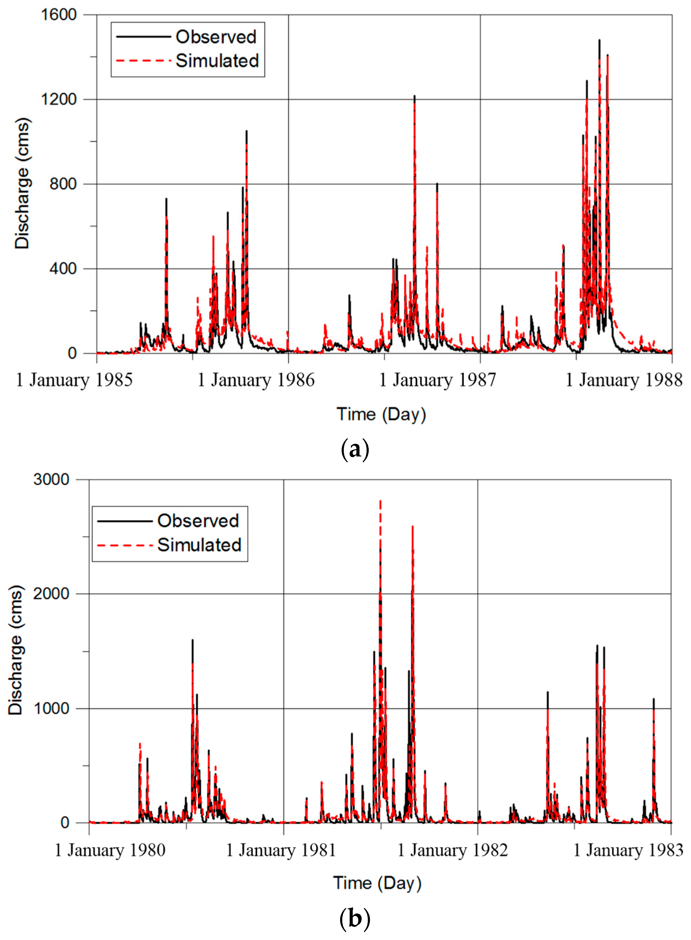
South Korea in particular has had unprecedented torrential rainfalls since 1998, including rainfalls of 500 mm/day in the Imjin River basin and 870 mm/day in Gangneung Province. As the annual average rainfall for South Korea is about 1280 mm, the rainfall record of 870 mm/day was about 65% of the annual average. With regard to drought, the Korean peninsula faced a severe drought during 2014–2015. The total annual precipitation in these years was temporally less than 35%–50% of the long-term average from 1973 to 2015. As a result, the local government imposed water use restrictions in eight cities on the west coast of South Korea in 2015. The establishment of a monthly or seasonal water resources’ management strategy is therefore necessary in South Korea. Additionally, it is necessary to quantify the impacts of the two types of factors on hydrological responses in South Korea over different time scales. Hydrological modeling is therefore indispensable to the assessment of these impacts at higher time resolutions. In this study, the SWAT (Soil and Water Assessment Tool) model was used to investigate the effects of climate change and human activities on hydrological responses in two catchments at monthly, seasonal and annual time scales. In particular, the six hydrological sensitivity methods employed at an annual scale can be used to verify the results of the hydrological model-based approach.

2. Study Area and Data Characteristics

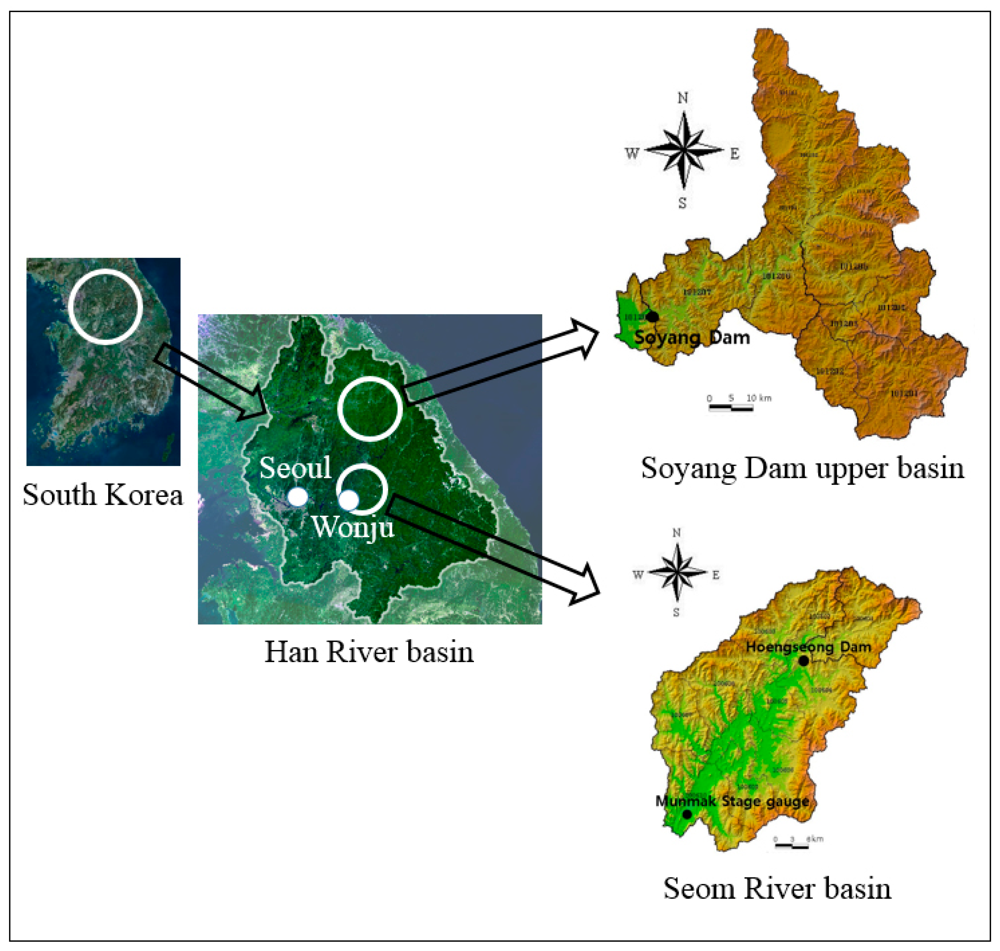
Two catchments undergoing a change in population and land use were selected to compare the relative impacts of climate change and human activities. One was the Soyang Dam upper basin (128°15′ E~128°56′ E, 38°13′ N~38°24′ N), located in northeastern South Korea (Figure 1). Soyang Dam was constructed in 1973 and has played an important role in preventing floods and supplying water to the area around the Korean capital, Seoul. This basin is 2703 km2 in area and consists of three sub-basins, Inbuk (923.8 km2), Naerin (1069.3 km2) and Soyang (709.9 km2). The other catchment selected was the Seom River basin (128°02′ E~128°13′ E, 37°56′ N~37°89′ N), located about 150 km south of the Soyang Dam upper basin (Figure 1). The area of this basin is 1491 km2, and Hoengseong Dam, built in 2001, is located on the upper site. Hoengseong Dam is located at an elevation of 180.0 m and is 48.5 m in height and 205 m in length. This dam has 87 million m3 of total storage, 119.5 million m3/year of water supply capacity and 9.5 million m3 of flood control capacity. The regulation of Soyang Dam to mitigate flood and drought cannot change hydrological responses in the Soyang Dam upper basin because the dam is located at the outlet of the basin, while the regulation of the Hoengseong Dam can significantly regulate streamflow at the outlet of its basin because it is located at the upper site of the basin. However, the regulation of the Hoengseong Dam might effectively impact short-term runoff change.
Meteorological and hydrological data were collected at the two basins to assess the effects of climate change (www.wamis.go.kr). The precipitation datasets at the two basins were collected, but potential evapotranspiration datasets at the two basin were calculated by the Penman–Monteith method [37,38]. Therefore, the net radiation, mean daily temperature and wind speed datasets in the two basins also were collected to perform the Penman–Monteith method. In the Soyang Dam upper basin, data for total annual rainfall and inflow into the Soyang Dam during 1974–2014 were collected. In the Seom River basin, data for total annual rainfall during 1974–2014 and runoff at Munmak gauge station during 1994–2014 were collected. The data were collected from 1994 because the gauge station was installed in 1993. Meanwhile, the role of human activities was calculated from the change of population and increased impervious area due to urban development. Therefore, data for population growth during 1966–2011 and the area of the impervious layer during 1975–2011 were collected at the two catchments. 
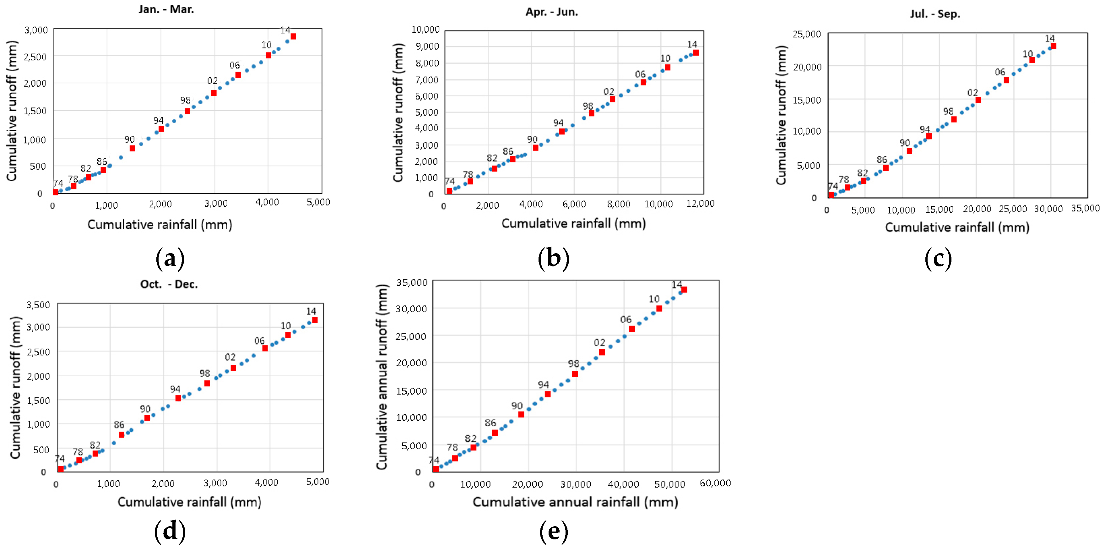
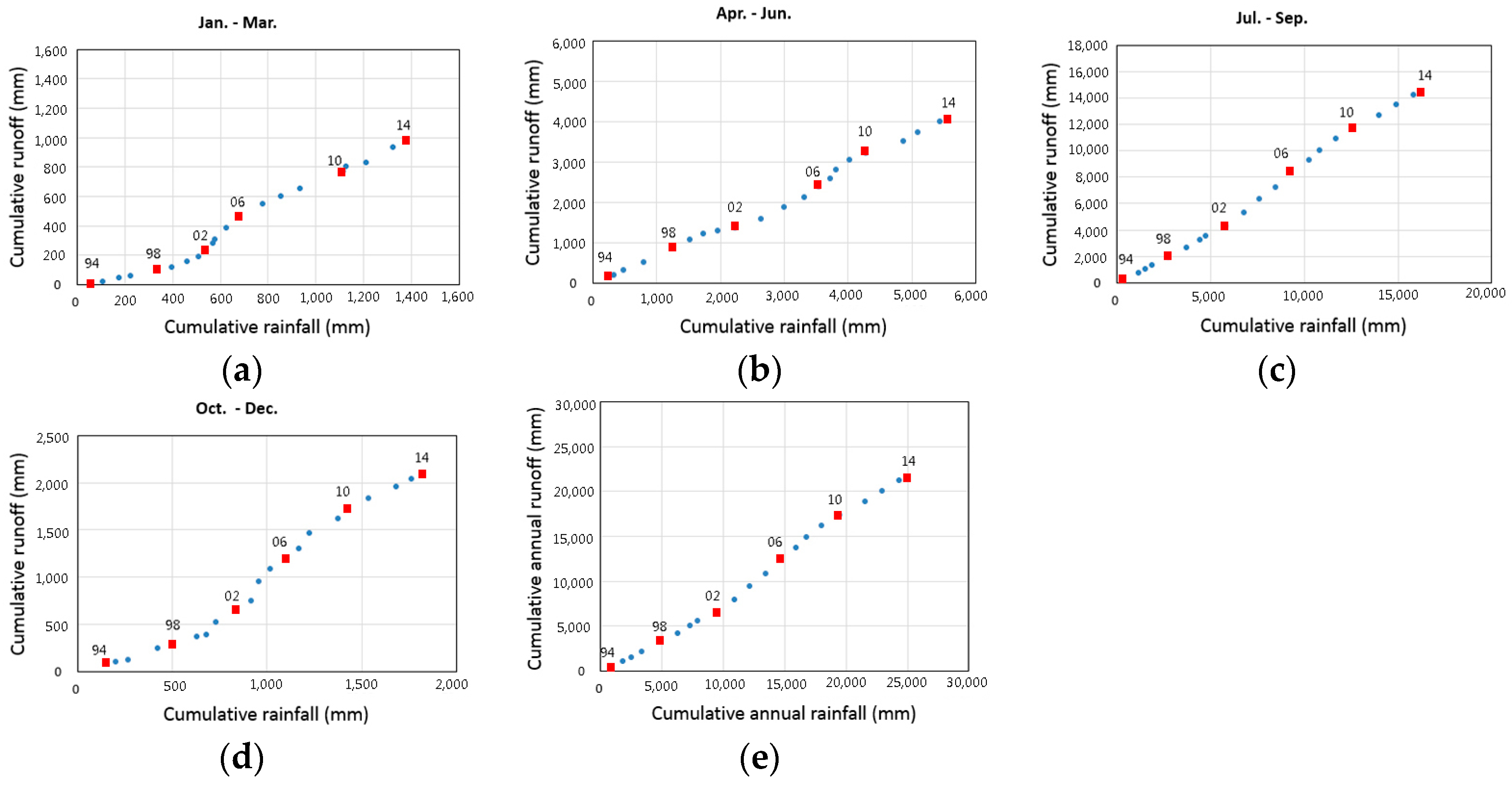
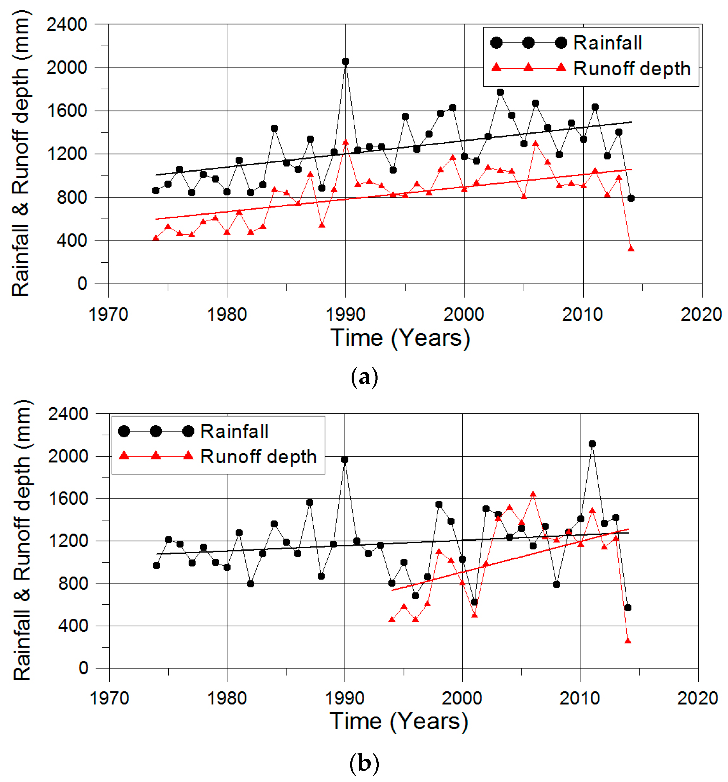
Figure 2 shows the total annual rainfall and runoff depth for the two catchments. The averages for rainfall over 41 years in the Soyang Dam upper basin and the Seom River basin were 1249.8 mm and 1175.4 mm, respectively. The black and red lines in Figure 2 roughly show the trends in the collected data by linear regression. The trends in total annual rainfall at the two catchments were similar to each other, while the trend in the runoff depth (= runoff volume/basin area) in the Seom River basin is more severe than that in the Soyang River basin.
In this study, a Mann–Kendall test based on a statistical hypothesis test was performed to more closely investigate trends in collected annual rainfall. The Mann–Kendall test is a non-parametric test used to identify trends in time series. One benefit of this test is that the data need not conform to any particular probability distribution. When x j and x k in time series X = [ x 1 , x 2 , , x n ] are independent, the statistics S and signs can be defined as the following equations. The statistical hypothesis test is performed to find the p-value using Z M K and significance level, α . Table 1 shows the results of the Mann–Kendall non-parametric test, at the 5% significance level, for total annual rainfall in the selected basins. In this table, all annual averages showed increasing trends. It can therefore be concluded that climate change was similar in the two basins.
S = k = 1 n 1 j = k + 1 n sgn ( x j x k ) ,   sgn ( x j x k ) = { 1 0 1 i f i f i f ( x j x k ) ( x j x k ) ( x j x k ) > 0 = 0 < 0
Z M K = { ( S 1 ) / V a r [ S ] 0 ( S + 1 ) / V a r [ S ] i f i f i f   S > 0   S = 0   S < 0
However, the runoff depth in the Seom River basin was considerably higher than that in the Soyang Dam upper basin. Figure 2b shows that runoff depth was about twice as high during 2003–2013 as it was before 2004. This abrupt change in runoff depth was caused by the increase of impervious area and the operation of the Hoengseong Dam, which was built in 2001. Especially the regulation of the Heonseong Dam might effectively impact short-term runoff change. It was also necessary to evaluate population change and change in impervious area. Figure 3 shows the change in population and impervious area in the two basins. Figure 3a shows that the population in the Soyang Dam upper basin decreased during 1966–2011, while the population in the Seom River basin increased significantly after 1995. Additionally, as Figure 3b shows, the impervious area caused by urban development increased dramatically after 1990 in the Seom River basin, while the increase in the Soyang River basin was relatively small. We therefore predicted that the hydrological responses in the Seom River basin would be impacted significantly by human activities due to the construction of the Hoengseong Dam, population growth and the expansion of impervious area.

3. Methodology

3.1. Framework for Quantifying the Relative Impact

The hydrological responses, such as runoff, can be changed by climate change and human activities, and this process can be modeled by the following equation [39].
Q = f ( C , H )
Here, Q is runoff; C and H are variables to represent climate change and human activities, respectively. Using a first-order approximation to Equation (3), Equation (4) can be derived as [39]:
Δ Q = Q C Δ C + Q H Δ H = Δ Q C + Δ Q H
Here, Δ Q is total change in runoff; Δ Q C and Δ Q H represent changes in runoff due to climate change and human activities, respectively. Among two variables ( Δ Q C and Δ Q H ), only one variable needs to be identified to solve Equation (4) because total runoff change, Δ Q , is already a known variable from the observed runoff. Wang et al. [25] regarded these two variables as independent, although climate change and human activities interact with each other in the real world. Therefore, in this study, the independent assumption was applied to all calculating processes.
The change in runoff due to climate variability is likely to proceed gradually, but the change due to human activities shows abrupt change. When climate change and human activities impact runoff, the schematic tendency can be depicted as Figure 4.
In Figure 4, a change point (or many change points) can occur because of abrupt change by human activities. The natural period (hereafter P1) is defined as the period impacted by only the climate change factor, and the impacted period (hereafter P2) is defined as the period impacted by climate change and human activities in this study. Firstly, Δ Q can be calculated simply by the difference between Q ¯ o b s 1 and Q ¯ o b s 2 because the observed runoff in all periods was already collected from a basin of interest. Consequently, quantifying the relative impacts due to the two types of factors can be performed by estimation of Δ Q C or Δ Q H . Especially, the detection of a change point through reasonable methods should be prior to calculating Δ Q C or Δ Q H . Furthermore, some reasonable approaches for calculating Q ¯ s i m 2 should be elicited.

3.2. Detection of a Change Point

A change point is a specific location of time, and this point can occur by abrupt change in a time series. The double mass curve can be used to detect change points roughly. This curve is a plot of the accumulated values of one variable against the accumulated values of the other value during a concurrent period. A change in the gradient of the curve may indicate that the original relationship between two variables was broken [40]. The double mass curve has been used to detect a change due to human activities [34,35,41].
Furthermore, Pettitt’s test and the Bayesian change point analysis can be used to detect a change point more certainly. Pettitt’s test [42] is a sort of non-parametric trend test to detect a change point. This test is commonly applied to detect a single change point in hydrological or meteorological time series. The null hypothesis in this test is H 0 : some T variables follow one or more distributions that have the same location parameter (so, no change); and then, the alternative hypothesis is H A : a change point exists in the time series. The non-parametric statistics by Pettitt is defined as Equation (5). The change point is detected at K T , provided that the statistics is significant. The significance probability of K T is approximated as Equation (6).
K T = max | U t , T | ,   U t , T = i = 1 t j = t + 1 T sgn ( x i x j )
p 2 exp ( 6 K T 2 T 3 + T 2 )
Another change point test is Bayesian change point analysis (BCP analysis), and its advantage is to detect many change points through multiple change point analysis at once. Let us assume that { x i } i = 1 i = n is a sequence of observed time series with the probability density functions p 1 ( x ) , p 2 ( x ) , , p n ( x ) . Therefore, for a sequence of n independent random variables X = ( X 1 , X 2 , , X n ) , the change point model can be described by Equation (7). In Equation (7), the parameter in probability density functions θ 1 θ 2 , , θ n and the change points τ 1 , τ 2 , , τ n 1 are unknown. Therefore, this time series can be divided into n homogenous groups if the locations of change points are determined. Thus, each part of the sequence of random variables is distributed as statistical distributions, which belong to the same class, but with a different unknown parameter θ , such as the mean and variance. The BCP analysis uses the Bayesian framework to detect some change point in Equation (7).
X i ~ { p 1 ( x ) = p ( x i | θ 1 ) , 1 i τ 1 p 2 ( x ) = p ( x i | θ 2 ) , τ 1 < i τ 2 p n ( x ) = p ( x i | θ n ) , τ n 1 < i τ n
Especially, Barry and Hartigan [43] used the product partition model, which assumes that the probability of any partition is proportional to a product of prior cohesions. Chib [44] formulated the multiple change point model using the Markov process with transition probabilities. Recently, the BCP analysis has been applied to detect some abrupt change in hydrological or meteorological time series [45,46,47]. The double mass curve, Pettitt’s test and the BCP analysis were used to detect a change point in observed runoff time series in this study. Furthermore, the BCP package developed by Erdman and Emerson [48] on R was used.

3.3. Generation of Simulated Runoff by the Hydrological Model

A hydrological model can be used to simulate Q ¯ s i m 2 in Figure 4. The basic concept is that the hydrological models simulate a condition that would have occurred without human activities, this natural condition in P1, which would be only a result of climate change factors. Therefore, it is necessary that the selected hydrological model should be firstly calibrated on observed runoff in the natural period, P1. After calibration to P1, the calibrated parameters in the selected hydrological model should be used to simulate runoff in the impacted period, P2. Finally, the quantitative impact due to human activities can be calculated as Equation (8). Furthermore, it is possible to calculate the quantitative impact due to climate change, Δ Q C , from Equation (4).
Δ Q H = Q ¯ o b s 2 Q ¯ s i m 2
The SWAT model was selected to simulate the runoff in P1 and P2 in this study. This model is a continuous, semi-distributed, physically-based hydrological model developed by the U.S. Department of Agriculture-Agriculture Research Service (USDA-ARS). Furthermore, this model simulates the impact of land management strategy on water, sediment and various water pollutants. The SWAT model is performed on hydrological response units, which are sub-units of sub-basins with unique combinations of soil and land use characteristics. The SWAT model requires spatial data inputs, including topography, climate, land use and soil. For a further description of the theoretical background, the study of Neitsch et al. [49] can be referenced. Furthermore, the ParaSol (Parameter Solution) procedure in the SWAT-CUP (SWAT-Calibration and Uncertainty Procedures) was used to calibrate in this study automatically. Among the various algorithms such as Particle Swarm Optimization (PSO), Sequential Uncertainty FIttting-2 (SUFI-2), Markov Chain Monte Carlo (MCMC), Generalized Likelihood Uncertainty Estimation (GLUE) in the SWAT-CUP, the SUFI-2 algorithm was used. For more detailed information on the SUFI-2 algorithm, the report of Abbaspour [50] can be referenced.

3.4. Generation of Simulated Runoff by Hydrological Sensitivity

Hydrological sensitivity means the change in mean annual runoff in response to the change in mean annual precipitation and potential evapotranspiration ( P E T ). Water balance can be described by runoff, precipitation and actual evapotranspiration ( A E T ) as Equation (9).
P = Q + A E T + Δ S
Here, P , Q and A E T are precipitation, runoff and actual evapotranspiration during a period, respectively. Furthermore, Δ S is the change in storage in a basin. However, in a long-term period (more than about 10 years) with an annual time scale, Δ S can be neglected because its summation can be assumed as zero [51].
Meanwhile, in an analysis of water resources’ modeling, the Budyko curve has been frequently used to simulate evaporation. The Budyko curve based on Budyko’s assumption [36] is developed by two balance equations on water and energy. One is Equation (9), and the other is Equation (10), to represent the energy balance in a basin [52].
N = L × A E T + H + Δ G
Here, N , L , H and Δ G are the net radiation, the latent heat for evaporation, the sensible heat flux during a period and the change of net ground heat flux, respectively. Furthermore, Δ G can be assumed as zero for the same reason as Δ S [51]. After elimination of Δ S and Δ G in Equations (9) and (10), it is assumed that P E T = N / L and γ = H / ( L × A E T ) . By dividing Equation (10) by Equation (9), Equation (11) can be derived simply.
P E T P = A E T P + A E T × γ P = A E T P ( 1 + γ ) = ϕ
Here, γ and ϕ are called the Bowen ratio and aridity index. Because the Bowen ratio can be assumed as a function of the aridity index [51], γ = f ( ϕ ) , Equation (11) can be finally rearranged as Equation (12).
A E T P = ϕ 1 + f ( ϕ ) = F ( ϕ )
Here, F ( ϕ ) is called the Budyko curve equation. Many studies have been performed to find F ( ϕ ) using actual evapotranspiration and precipitation time series of more than 10 years on various regions. The commonly used 5 functions were developed by Schreiber [52], Ol’dekop [53], Pike [1], Budyko [36] and Fu [54]. The estimated functions are described in Table 2.
Therefore, the potential evapotranspiration, P E T , should be estimated by Equation (11) to determine the aridity index, ϕ . In this study, the evapotranspirations, P E T s , in Soyang Dam upper basin and Seom River basin were estimated by the Penman–Monteith method. After calculating the aridity index, ϕ , in the basin of interest, the actual evapotranspiration, A E T , can be calculated by the various types of Budyko curves. Especially, Zhang et al. [55] developed another type of Budyko curve using mean annual evapotranspiration to vegetation. Equation (13) is the relationship developed by Zhang et al. [55].
A E T P = F ( ϕ ) = 1 + ω ( P E T / P ) 1 + ω ( P E T / P ) + ( P E T / P ) 1
Here, ω is a plant-available water coefficient related to vegetation type. In this study, the plant-available water coefficient, ω , was calibrated by the actual evapotranspiration, A E T , in Equation (9).
The hydrological sensitivity, which means perturbation in runoff, Δ Q can be derived by the water balance equation (Equation (9)). Especially, in the hydrological sensitivity approach, Δ Q can be assumed Δ Q C because Δ Q is impacted by only meteorological variables, such as precipitation and actual evapotranspiration. Therefore, Δ Q can be denoted by Δ Q C in Equation (4). Finally, the perturbation of Equation (9) without human activities can be described by Equation (14).
Δ Q C = Δ P Δ A E T
Here, Δ Q C , Δ P and Δ A E T are the change in runoff due to only climate change, the change in precipitation and the change in actual evapotranspiration.
Koster and Suarez [56] developed a relationship between actual evapotranspiration and the Budyko curve function. The total derivative to Equation (12) ( A E T = P × F ( ϕ ) ) is described as Equation (15). Furthermore, the total derivative to the aridity index function ( ϕ = P E T / P ) is represented by Equation (16).
d ( A E T ) = F ( ϕ ) d P + P F ( ϕ ) d ϕ Δ A E T = F ( ϕ ) Δ P + P F ( ϕ ) Δ ϕ
d ϕ = 1 P d ( P E T ) P E T P 2 d P Δ ϕ = 1 P Δ ( P E T ) P E T P 2 Δ P
By substituting Equation (16) for Equation (15) and rearranging,
Δ A E T = [ F ( ϕ ) ϕ F ( ϕ ) ] Δ P + F ( ϕ ) Δ P E T
Furthermore, by substituting Equation (17) for Equation (14),
Δ Q C = [ 1 F ( ϕ ) + ϕ F ( ϕ ) ] Δ P F ( ϕ ) Δ P E T = α Δ P + β Δ P E T
Because Equation (9) can be rearranged by A E T = P × F ( ϕ ) :
Q = P ( 1 F ( ϕ ) )
Dividing Equation (18) by Equation (19) and using P = P E T / ϕ , Equation (20) is derived as:
Δ Q C = Δ P P Q ( 1 + ϕ F ( ϕ ) 1 F ( ϕ ) ) + Δ P E T P E T Q ( ϕ F ( ϕ ) 1 F ( ϕ ) ) = ε P Δ P P Q + ε P E T Δ P E T P E T Q
Here, ε P and ε P E T are called the elasticity coefficient of precipitation and potential evapotranspiration, and ε P + ε P = 1 . Finally, Equation (20) can be used to estimate the change in runoff due to only climate factors. Furthermore, in Equation (18), the coefficients α and β were estimated by Li et al. [57].
α = 1 + 2 x + 3 ω x ( 1 + x + ω x 2 ) 2 , β = 1 + 2 ω x ( 1 + x + ω x 2 ) 2
Here, ω is the plant-available water coefficient in Zhang’s Budyko-based method [55], and x = P E T / P . In this study, the 5 Budyko-based methods (Table 2), by calculating the elasticity coefficients, were used. Furthermore, Zhang’s method using coefficients α and β was used.

4. Applications

4.1. Detection of Change Points over Different Time Scales

In this study, the data for daily precipitation and observed runoff depth during 1974–2014 in the Soyang Dam upper basin and the data for the same factors during 1994–2014 in the Seom River basin were used to detect a change point. The daily data were used only at the seasonal and annual time scales to detect change points, because change point detection at the monthly scale is very time consuming. It was therefore assumed that the monthly change points in a season were identical. The seasonal data were divided into four sections: January–March (JFM), April–June (AMJ), July–September (JAS) and October–December (OND) according to the meteorological characteristics of South Korea.
Figure 5a–e shows the results obtained using the double mass curve technique in the Soyang Dam upper basin. The relationship between straight lines with slightly different slopes for the Soyang Dam upper basin is shown. It can therefore be concluded that the change points were located at 1987–1988 (JFM), 1988–1989 (AMJ), 1982–1983 (JAS) and 1983–1984 (OND). At the annual time scale, the change point was located at 1983–1984. We can therefore conclude that the runoff characteristics in JFM–AMJ were different from those in JAS–OND.
In Figure 6a–e for the Seom River basin, the slope lines were clearly changed around 2002–2003. We can conclude that the change points were located at 2000–2001 (JFM), 2002–2003 (AMJ), 2002–2003 (JAS) and 2000–2001 (OND). At the annual time scale, the change point was located at 2001–2002. The change in runoff in the Seom River basin might result from the regulation of the Hoengseong Dam, built on the upper site of this basin in 2001.
It is very important to separate the climate change and human activities contributing to these results. Pettitt’s test at the 5% significance level and the BCP (Bayesian change point) analysis using the posterior mean change with the probability of change were therefore performed to more accurately locate the change points in the two selected basins. Table 3 shows the results of Pettitt’s test, and Table 4 shows the results of the BCP analysis. Apparently, the results from the three techniques were very similar. The seasonal change points drawn from all results are summarized in Table 5.

4.2. Calibration and Verification of the SWAT Model

The two approaches, the hydrological model method and the hydrological sensitivity method, were used to quantify the relative impacts of climate change and human activities in the two basins. The SWAT models were developed for the selected basins to simulate the runoff during the impacted period, P2. It is therefore necessary to calibrate and validate the SWAT models during the natural period, P1. Additionally, the calibration should be performed for two distinct periods in the Soyang Dam upper basin because the change points in JFM–AMJ and those in JAS-annual were different.
Therefore, the calibration years were selected to consider the detected change points in two basins. In the Soyang Dam upper basin, the period during 1985–1987 was used to calibrate for JFM and AMJ. The period during 1976–1978 was used to calibrate for JAS, OND and annual. After calibration using SWAT-CUP, two calibrated models were validated for the same period, 1980–1982. In the case of the Seom River basin, all detected change points were located around 2001–2003. The period during 1997–1999 and the period during 1994–1995 were therefore used to calibrate and validate the SWAT model. In addition, the first year in all calibration procedures was chosen as the warm up period to eliminate initial bias. The objective function in the calibration process was Nash–Sutcliffe efficiency (NSE) [58]. Furthermore, the validations of model performance after calibration were checked using NSE. The NSEs for JFM–AMJ and JAS-annual in calibration and validation were 0.79 and 0.77 and 0.82 and 0.84, respectively, in the Soyang Dam upper basin. In the Seom River basin, the NSEs in calibration and validation were 0.78 and 0.81, respectively. We therefore conclude that the SWAT models in the two basins can simulate the runoff in the impacted period, P2, with reasonable accuracy. Figure 7a,b show examples of the calibration and validation results for JFM–AMJ in the Soyang Dam upper basin.

4.3. Verification of the Hydrological Model Approach

The annual results from the hydrological model approach were validated and compared with the results from the six hydrological sensitivity methods before being analyzed at the monthly and seasonal time scales. The six methods used were the Budyko curve functions developed by Schreiber [52], Ol’dekop [53], Pike [1], Budyko [36], Fu [54] and Zhang [55]. Firstly, the elasticity coefficients for five Budyko curve functions and Zhang’s coefficients were estimated.
In this study, the potential evapotranspiration, P E T , was calculated using the Penman–Monteith method [37,38]. The plant-available water coefficient in Zhang’s ω was estimated to be 0.7. Table 6 shows the estimated elasticity coefficients for five Budyko-based methods and the coefficients for Zhang’s method. The annual runoff changes caused by climate change, Δ Q C , were first calculated from the estimated coefficients and Equations (18), (20) and (21). After calculating Δ Q C , we obtained the runoff change caused by human activities, Δ Q H , from water balance equations. Table 7 and Table 8 show the results obtained from the six Budyko-based methods and from the hydrological modeling approach, on an annual scale. These results can be used to verify the results obtained from the hydrological modeling approach.
In the Soyang Dam upper basin (Table 7), the average of Δ Q C calculated from the six Budyko-based methods (69.1%) was very similar to Δ Q C calculated from the hydrological modeling approach (71.5%). In the Seom River basin (Table 8), the average of Δ Q C calculated from the six Budyko-based methods (27.0%) and Δ Q C calculated from the hydrological modeling approach (27.6%) were also very similar. It can therefore be concluded that the results obtained from the hydrological modeling approach over different time scales were reasonable accurate for the two basins.

4.4. Results over Different Time Scales Obtained Using Hydrological Modeling

The impacts of climate change and human activities on hydrological responses were separated by means of the hydrological modeling method using the SWAT model. Firstly, the total changes in runoff, Δ Q , were calculated from the difference between the mean of the observed runoff in the natural period, P1, and the mean of the observed runoff in the impacted period, P2. After calculating the difference in runoff before and after the detected change point, the runoff changes caused by human activities, Δ Q H , were calculated from the difference between the observed and the simulated runoff in the impacted period, P2. Finally, the runoff changes caused by climate change, Δ Q C , were obtained using Equation (4). This procedure was performed at the annual, seasonal and monthly time scales for the two basins.
Table 9 and Table 10 show the results for the runoff changes ( Δ Q ), the runoff changes caused by human activities ( Δ Q H ), the runoff changes caused by climate change ( Δ Q C ) and their proportions over the different time scales in the two basins. In the Soyang Dam upper basin (Table 9 and Figure 8a), the total change in runoff is 526 mm at the annual time scale. The change in runoff caused by human activities is 150.1 mm (28.5%), and the change caused by climate change is 376 mm (71.5%). The ratios of change caused by human activities vs. climate change for JFM, AMJ, JAS and OND were 22.4:77.6, 26.4:73.6, 31.1:69.0 and 26.7:73.3, respectively. We therefore conclude that the effects of human activities for JFM, AMJ and OND were almost identical. However, for JAS, the proportion of change due to human activities was about 6% higher than the average of the other seasons. We used the monthly time scale to analyze these results in detail. We found that the proportions of change caused by human activities were slightly higher in AUG and SEP than in other months (Figure 8a). We therefore suggest that the runoff in summer has increased slightly due to deforestation for the development of vegetable farms in the mountains and a slight enlargement of the impervious layer. Finally, our results suggest that the impacts of climate change have been stronger than those of human activities in the Soyang Dam upper basin.
In the Seom River basin (Table 10 and Figure 8b), the total change in runoff was 214 mm at the annual time scale. The change in runoff caused by human activities was 154.9 mm (72.4%), and that of climate change was 59.0 mm (27.6%). The proportions for JFM, AMJ, JAS and OND caused by human activities vs. climate change were 109.1:−9.1, 69.7:30.3, 65.7:34.3 and 95.3:4.7, respectively. This suggests that the impacts of human activities have been stronger in this basin than those of climate change. In particular, the proportions of impacts of human activities for JFM and OND were about 40% higher than those for AMJ and JAS. Additionally, the proportions of human impacts on January, February, November and December were higher than 120%. This suggests that the streamflow at Munmak gauge station has been severely affected by outflow from the Hoengseong Dam in the winter season.
Figure 9a,b shows a summary and comparison of the results obtained for the two selected basins using the hydrological modeling approach at the annual scale. In the Soyang Dam upper basin, the rainfall loss before 1983 can be estimated to be 467.7 mm. Additionally, the rainfall difference (370 mm) was almost identical to Δ Q C using the SWAT model (376.0 mm). We therefore conclude that the rainfall difference (370.0 mm) between P1 and P2 has caused most of the runoff increase associated with climate change, because the change in impervious area was insignificant in the Soyang Dam upper basin. Additionally, in the Seom River basin, the rainfall loss was 332.5 mm during 1994–2002, but this value might have been decreased during 1994–2001 due to increased impervious area. We predict that this effect might be reflected in human activities. From these figures, it is evident that the changes in hydrological responses of the two selected basins due to climate change and human activities were very different from each other.

5. Conclusions

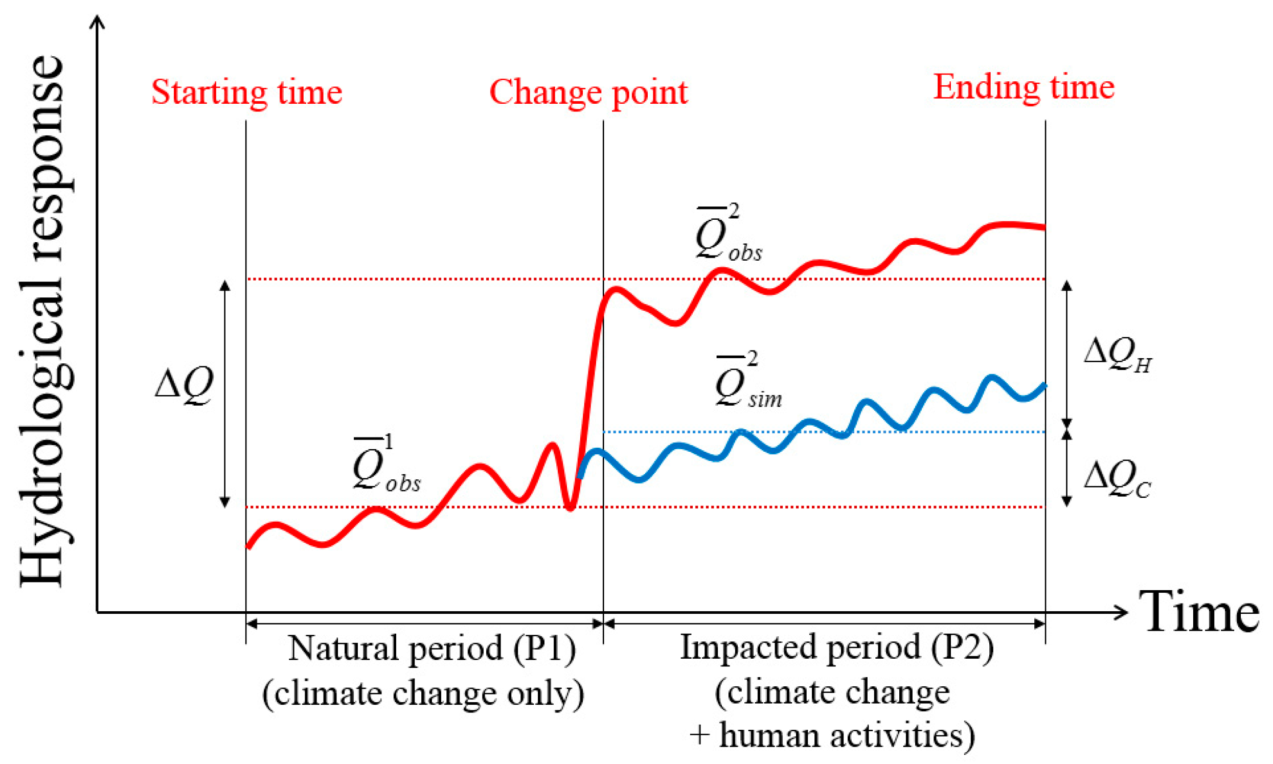
The hydrological variability caused by climate change and regional human activities should be quantitatively analyzed and managed because it affects all living things, including humans, in a basin. It is necessary that the relative impacts on the hydrological responses of climate change and human activities be separated and quantitatively understood in order to establish an appropriate water resources planning strategy. In particular, the impacts of the two types of factors should be evaluated over different time scales in watersheds where precipitation is unevenly distributed at the annual scale, as it is in South Korea, because water resources’ plans to manage flood and drought should be established at the monthly or seasonal scale. However, only a few studies analyzing the impacts of the two types of factors at various time scales have been conducted.
In this study, we employed two approaches (the hydrological model based method using the SWAT model and hydrological sensitivity-based methods using the six Budyko curve functions) to quantitatively assess the relative impacts of climate change and human activities at monthly, seasonal and annual time scales. Two basins, the Soyang Dam upper basin and the Seom River basin, were selected for comparison based on population growth and change in land use. Firstly, trend analyses using rainfall and runoff depth were performed using the Mann–Kendall nonparametric test. All annual averages for rainfall in the two basins showed a slight increasing trend, but the runoff depth in the Seom River basin showed a significant increasing trend. Furthermore, this study detected change points using the double mass curve, Pettitt’s test and the BCP analysis. For the hydrological model-based approach, the SWAT model should be calibrated and validated in the natural period. After calibration, the annual results obtained from the hydrological model method were validated using the results from the six hydrological sensitivity methods. The six Budyko functions developed by Schreiber, Ol’dekop, Pike, Budyko, Fu and Zhang were used to estimate the changes caused by climate change.
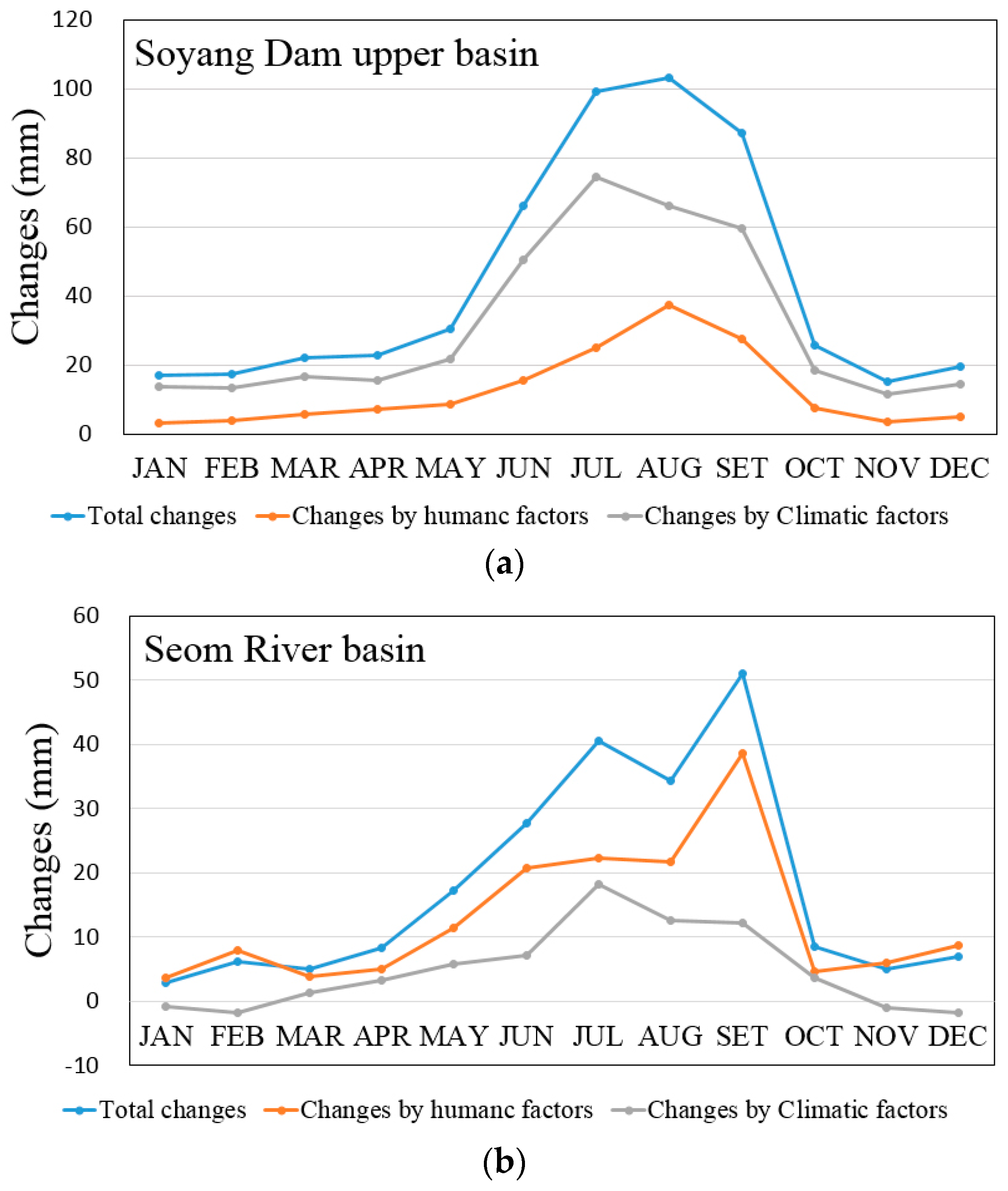
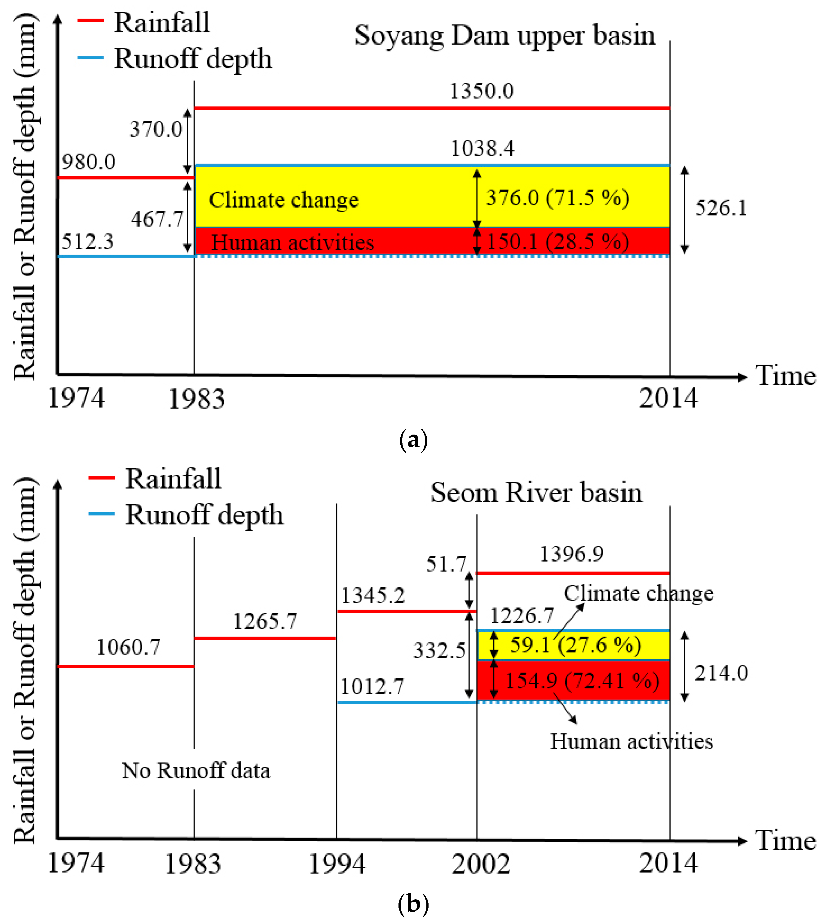
We concluded that the results obtained from the hydrological modeling approach at the different time scales were reasonably accurate for the two basins. The results obtained from the hydrological model method at the monthly, seasonal and annual time scales were therefore used to identify the causes of change in the two basins. In the Soyang Dam upper basin, the change in runoff caused by human activities is 28.5%, and that caused by climate change is 71.5%, at the annual scale. We also found that the proportion of change due to human activities for JAS was slightly higher than the average of the proportions for other seasons. Through monthly analysis, it can be shown that the proportions for AUG and SEP were slightly higher than for other months. In the Seom River basin, the change in runoff caused by human activities is 72.4%, and that caused by climate change is 27.6%. Additionally, the proportions of change caused by human activities for the winter seasons (JFM and OND) were significantly higher than for other seasons. In particular, the proportions of change caused by human activities for JAN, FEB, NOV and DEC were higher than 120%. Finally, our results suggest that the impacts of climate change have been stronger than those of human activities in the Soyang Dam upper basin, while the impacts of human activities have been stronger than those of climate change in the Seom River basin due to the increase of impervious area in the long-term aspect and regulation of the Hoengseong Dam in the short-term aspect.
In this study, we performed a quantitative assessment of the impacts of climate change and human activities on hydrological responses in two basins in South Korea. The causes of change identified in the two basins were significantly different. The procedure used in this study can be used as a reference for regional water resources planning and management on monthly and seasonal time scales. In the future, the uncertainty analysis in this procedure should be performed to establish more effective strategies for water resources’ management. The detailed analysis related to flood and low flow characteristics using water cycle components should be performed, and also, the independent assumption for two factors in this study should be revised to identify the interaction between climate change and human activities in future work.

Acknowledgments

This research was supported by Basic Science Research Program through the National Research Foundation (NRF) of Korea funded by the Ministry of Education (2014R1A1A2053328) and a grant (11-TI-C06) from the Advanced Water Management Research Program funded by the Ministry of Land, Infrastructure and Transport of the Korean government.

Author Contributions

Sangho Lee established the research direction and gave constructive suggestions. Sang Ug Kim performed the analysis in this study and also wrote the manuscript.

Conflicts of Interest

The authors declare no conflict of interest.

References

  1. Pike, J.G. The estimation of annual runoff from meteorological data in a tropical climate. J. Hydrol. 1964, 2, 116–123. [Google Scholar] [CrossRef]
  2. Nash, L.L.; Gleick, P.H. Sensitivity of streamflow in the Colorado basin to climatic changes. J. Hydrol. 1991, 125, 221–241. [Google Scholar] [CrossRef]
  3. Burn, D.H. Hydrologic effects of climatic change in West Central Canada. J. Hydrol. 1994, 160, 53–70. [Google Scholar] [CrossRef]
  4. Dam, J.C. Impacts of Climate Change and Variability on Hydrological Regimes; Cambridge University Press: Cambridge, UK, 1999. [Google Scholar]
  5. Abdul Aziz, O.I.; Burn, D.H.T. Trends and variability in the hydrological regime of the Mackenzie River basin. J. Hydrol. 2006, 319, 282–294. [Google Scholar] [CrossRef]
  6. Li, Z.L.; Xu, Z.X.; Li, J.Y.; Li, Z.J. Shift trend and step changes for runoff time series in the Shiyang River basin, northwest China. Hydrol. Process. 2008, 22, 4639–4646. [Google Scholar] [CrossRef]
  7. Shehadeh, N.; Ananbeh, S. The impact of climate change upon winter rainfall. Am. J. Environ. Sci. 2013, 9, 73–81. [Google Scholar] [CrossRef]
  8. Akurut, M.; Willems, P.; Niwagaba, C.B. Potential impacts of climate change on precipitation over Lake Victoria, East Africa, in the 21st Century. Water 2014, 6, 2634–2659. [Google Scholar] [CrossRef] [Green Version]
  9. Li, F.; Zhang, G.; Xu, Y.J. Assessing climate change impacts on water resources in the Songhua River basin. Water 2016, 8, 420. [Google Scholar] [CrossRef]
  10. Labat, D.; Godderis, Y.; Probst, J.L. Evidence for global runoff increase related to climate warming. Adv. Water Resour. 2004, 27, 631–642. [Google Scholar] [CrossRef] [Green Version]
  11. Milly, P.C.D.; Wetherhald, R.T.; Dunne, K.A.; Delworth, T.L. Increasing risk of great floods in a changing climate. Nature 2002, 415, 514–517. [Google Scholar] [CrossRef] [PubMed]
  12. Merz, B.; Vorogushyn, S.; Uhlemann, S.; Delgado, J.; Hundecha, Y. More efforts and scientific rigour are needed to attribute trends in flood time series. Hydrol. Earth Syst. Sci. 2012, 16, 1379–1387. [Google Scholar] [CrossRef]
  13. Petrow, T.; Merz, B. Trends in flood magnitude, frequency and seasonality in Germany in the period 1951–2002. J. Hydrol. 2009, 371, 129–141. [Google Scholar] [CrossRef]
  14. Mundelsee, M.; Börngen, M.; Tetzlaff, G.; Grünewald, U. No upward trends in the occurrence of extreme floods in central Europe. Nature 2003, 425, 166–169. [Google Scholar] [CrossRef] [PubMed]
  15. Tuteja, N.K.; Vase, J.; Teng, J.; Mutendeudzi, M. Partitioning the effects of pine plantations and climate variability on runoff from a large catchment in southeastern Australia. Water Resour. Res. 2007, 43, w08415. [Google Scholar] [CrossRef]
  16. Cheng, S.J.; Wang, R.Y. An approach for evaluating the hydrological effects of urbanization and its application. Hydrol. Process. 2002, 16, 1403–1418. [Google Scholar] [CrossRef]
  17. Dietz, M.E.; Clausen, J.C. Stromwater runoff and export changes with development in a traditional and low impact subdivision. J. Environ. Manag. 2008, 87, 560–566. [Google Scholar] [CrossRef] [PubMed]
  18. Du, J.; Qian, L.; Rui, H.; Zuo, T.; Zheng, D.; Xu, Y.; Xu, C.Y. Assessing the effects of urbanization on annual runoff and flood events using an integrated hydrological modeling system for Qinhuai River basin, China. J. Hydrol. 2012, 464–465, 127–139. [Google Scholar] [CrossRef]
  19. Li, Y.; Liu, C.; Zhang, D.; Liang, K.; Li, X.; Dong, G. Reduced runoff due to anthropogenic intervention in the Loess Plateau, China. Water 2016, 8, 458. [Google Scholar] [CrossRef]
  20. Seyoum, W.M.; Milewski, A.M.; Durham, M.C. Understanding the relative impacts of natural processes and human activities on the hydrology of the Central Rift Valley lakes, East Africa. Hydrol. Process. 2015, 29, 4312–4324. [Google Scholar] [CrossRef]
  21. Liu, D.; Chen, X.; Lian, Y.; Lou, Z. Impacts of climate change and human activities on surface runoff in the Dongjiang River basin of China. Hydrol. Process. 2010, 24, 1487–1495. [Google Scholar] [CrossRef]
  22. Jiang, S.; Ren, L.; Yong, B.; Singh, V.P.; Yang, X.; Yuan, F. Quantifying the effects of climate variability and human activities on runoff from the Laohahe basin in northern China using three different methods. Hydrol. Process. 2011, 25, 2492–2505. [Google Scholar] [CrossRef]
  23. Du, J.; He, F.; Zhang, Z.; Shi, P. Precipitation change and human impacts on hydrologic variables in Zhengshui River basin, China. Stoch. Environ. Res. Risk Assess. 2011, 25, 1013–1025. [Google Scholar] [CrossRef]
  24. Ye, X.; Zhang, Q.; Liu, J.; Xu, C.-Y. Distinguishing the relative impacts of climate change and human activities on variation of streamflow in the Poyang Lake catchment, China. J. Hydrol. 2013, 494, 83–95. [Google Scholar] [CrossRef]
  25. Wang, W.; Shao, Q.; Yang, T.; Peng, S.; Xing, W.; Sun, F.; Luo, Y. Quantitative assessment of the impact of climate variability and human activities on runoff changes: A case study in four catchment of the Haihe River basin, China. Hydrol. Process. 2013, 27, 1158–1174. [Google Scholar] [CrossRef]
  26. Ann, K.-H.; Merwade, V. Quantifying the relative impact of climate and human activities on streamflow. J. Hydrol. 2014, 515, 257–266. [Google Scholar]
  27. Zeng, S.; Xia, J.; Du, H. Separating the effects of climate change and human activities on runoff over different time scale in the Zhang river basin. Stoch. Environ. Res. Risk Assess. 2014, 28, 401–413. [Google Scholar] [CrossRef]
  28. Chang, B.; Li, R.; Zhu, C.; Liu, K. Quantitative impacts of climate change and human activities on water-surface area variations from the 1990s to 2013 in Honghu Lake, China. Water 2015, 7, 2881–2889. [Google Scholar] [CrossRef]
  29. Shirokova, L.; Vorobyeva, T.; Zabelina, S.; Klimov, S.; Moreva, O.; Chupakov, A.; Makhnovitch, N.; Gogolitsyn, V.; Sobko, E.; Shorina, N.; et al. Small Boreal Lake ecosystem evolution under the influence of natural and anthropogenic factors: Results of multidisciplinary long-term study. Water 2016, 8, 316. [Google Scholar] [CrossRef]
  30. Shrestha, R.R.; Peters, D.L.; Schnorbus, M.A. Evaluating the ability a hydrologic model to replicate hydro-ecologically relevant indicators. Hydrol. Process. 2014, 28, 4294–4310. [Google Scholar] [CrossRef]
  31. Vis, M.; Knight, R.R.; Pool, S.; Wolfe, W.J.; Seibert, J. Model calibration for estimating ecological flow characteristics. Water 2015, 7, 2358–2381. [Google Scholar] [CrossRef]
  32. Murphy, J.C.; Knight, R.R.; Wolfe, W.J.; Gain, W.S. Predicting ecological flow regime at ungaged sites: A comparison of methods. River Res. Appl. 2013, 29, 660–669. [Google Scholar] [CrossRef]
  33. Xiong, L.H.; Guo, S.L. Two-parameter water balance model and its application. J. Hydrol. 1999, 216, 111–123. [Google Scholar] [CrossRef]
  34. Huo, Z.; Feng, S.; Kang, S.; Li, W.; Chen, S. Effect of climate changes and water-related human activities on annual stream flows of the Shiyang river basin in arid north-west China. Hydrol. Process. 2008, 22, 3155–3167. [Google Scholar] [CrossRef]
  35. Zhang, S.; Lu, X.X. Hydrological responses to precipitation variation and diverse human activities in a mountainous tributary of the lower Xijiang, China. Catena 2009, 77, 130–142. [Google Scholar] [CrossRef]
  36. Budyko, M.I. Evaporation under Natural Conditions; Gidrometeorizdat: Leningrad, Russia, 1948. [Google Scholar]
  37. Penman, H.L. Natural evaporation from open water, bare soil and grass. Proc. R. Soc. Lond. Ser. A Math. Phys. Sci. 1948, 193, 120–145. [Google Scholar] [CrossRef]
  38. Monteith, J.L. Evaporation and Environment. In The State and Movement of Water in Living Organism: Proceedings of the 19th Symposium of the Society for Experimental Biology; Cambridge University Press: New York, NY, USA, 1965; pp. 205–234. [Google Scholar]
  39. Zhang, X.; Zhang, L.; Zhao, J.; Rustomji, P.; Hairsine, P. Responses of streamflow to changes in climate and land use/cover in the Loess Plateau, China. Water Resour. Res. 2008, 44, W00A07. [Google Scholar] [CrossRef]
  40. Searcy, J.K.; Hardison, C.H. Double-Mass Curves; USGS Water-Supply Paper 1541-B; U.S. Government Printing Office: Washington, DC, USA, 1960; pp. 31–66.
  41. Zhang, W.; Yan, Y.; Zheng, J.; Li, L.; Dong, X.; Cai, H. Temporal and spatial variability of annual extreme water level in the Pearl River Delta region, China. Glob. Planet. Chang. 2009, 69, 35–47. [Google Scholar] [CrossRef]
  42. Pettitt, A.N. A non-parametric approach to the change-point problem. Appl. Stat. 1979, 28, 126–135. [Google Scholar] [CrossRef]
  43. Barry, D.; Hartigan, J.A. A Bayesian analysis for change point problems. J. Am. Stat. Assoc. 1993, 88, 309–319. [Google Scholar] [CrossRef]
  44. Chib, S. Estimation and comparison of multiple change-point models. J. Econom. 1998, 86, 221–241. [Google Scholar] [CrossRef]
  45. Zhang, Q.; Xu, C.-Y.; Chen, X.; Lu, X. Abrupt changes in the discharge and sediment load of the Pearl River, China. Hydrol. Process. 2012, 26, 1495–1508. [Google Scholar] [CrossRef]
  46. Brulebois, E.; Castel, T.; Richard, Y.; Chateau-Smith, C. Hydrological response to an abrupt shift in surface air temperature over France in 1987/88. J. Hydrol. 2015, 531, 892–901. [Google Scholar] [CrossRef]
  47. Lee, S.; Kim, S.U. Comparison between change point detection methods with synthetic rainfall data and application in South Korea. KSCE J. Civ. Eng. 2016, 20, 1558–1571. [Google Scholar] [CrossRef]
  48. Erdman, C.; Emerson, J.C. bcp: An R package for performing a Bayesian analysis of change point problems. J. Stat. Softw. 2007, 23, 1–13. [Google Scholar] [CrossRef]
  49. Neitsch, S.L.; Arnold, J.G.; Kiniry, J.R.; Williams, J.R. Soil and Water Assessment Tool Theoretical Documentation Version 2009; Texas Water Resources Institute Technical Report No. 406; Texas A&M University System: College Station, TX, USA, 2011. [Google Scholar]
  50. Abbaspour, K.C. SWAT-CUP Calibration and Uncertainty Programs: A User Manual; Eawag: Dübendorf, Switzerland, 2013. [Google Scholar]
  51. Arora, V.K. The use of aridity index to assess climate change effect on annual runoff. J. Hydrol. 2002, 265, 164–177. [Google Scholar] [CrossRef]
  52. Schreiber, P. Über die Beziehungen zwischen dem Niederschlag und der Wasserführung der Flüsse in Mitteleuropa. Meteorol. Z. 1904, 21, 441–452. [Google Scholar]
  53. Ol’dekop, E.M. On evaporation from the surface of river basins. Trans. Meteorol. Obs. Univ. Tartu 1911, 4, 200. [Google Scholar]
  54. Fu, B.P. On the calculation of the evaporation from land surface. Chin. J. Atmos. Sci. 1981, 5, 23–31. (In Chinese) [Google Scholar]
  55. Zhang, L.; Dawes, W.R.; Walker, G.R. The response of mean annual evaportranspiration to vegetation changes at catchment scale. Water Resour. Res. 2001, 37, 701–708. [Google Scholar] [CrossRef]
  56. Koster, R.D.; Suarez, M.J. A simple framework for examining the interannual variability of land surface moisture fluxes. J. Clim. 1999, 12, 1911–1917. [Google Scholar] [CrossRef]
  57. Li, L.J.; Zhang, L.; Wang, H.; Wang, J.; Yang, J.W.; Jiang, D.J.; Li, J.Y.; Qin, D.Y. Assessing the impact of climate variability and human activities of streamflow from the Wuding River basin in China. Hydrol. Process. 2007, 21, 3485–3491. [Google Scholar] [CrossRef]
  58. Nash, J.E.; Sutcliffe, J.V. River flow forecasting through conceptual models part I: A discussion of principles. J. Hydrol. 1970, 10, 282–290. [Google Scholar] [CrossRef]
Figure 1. Configuration map of the two selected basins.
Water 09 00034 g001
Figure 2. Rainfall and runoff depth in two basins. (a) Soyang Dam upper basin; (b) Seom River basin.
Water 09 00034 g002
Figure 3. Population and impervious area in two basins. (a) Populations; (b) impervious area.
Water 09 00034 g003
Figure 4. Schematic diagram to quantify relative impacts by two factors.
Water 09 00034 g004
Figure 5. Detection of change point in Soyang Dam upper basin (double mass curve). (a) JFM; (b) AMJ; (c) JAS; (d) OND; (e) annual. The numbers in figures mean years (e.g., 14 means 2014 year).
Water 09 00034 g005
Figure 6. Detection of change point in Seom River basin (double mass curve). (a) JFM; (b) AMJ; (c) JAS; (d) OND; (e) annual. The numbers in figures mean years (e.g., 14 means 2014 year).
Water 09 00034 g006
Figure 7. Calibration and validation of the Soil and Water Assessment Tool (SWAT) model in the Soyang Dam upper basin. (a) Calibration on JFM and AMJ; (b) validation on JFM and AMJ.
Water 09 00034 g007
Figure 8. Estimated monthly changes. (a) Soyang Dam upper basin; (b) Seom River basin.
Water 09 00034 g008
Figure 9. Summary of the hydrological modeling method on an annual scale. (a) Soyang Dam upper basin; (b) Seom River basin.
Water 09 00034 g009
Table 1. Results of the Mann–Kendall trend test in the two basins.
BasinsM–K Test Statisticsp-ValueDecision
Soyang Dam upper basin3.17850.0015trend
Seom River basin3.02520.0025trend
Table 2. Commonly-used Budyko curves.
Name of Function F ( ϕ )
Schreiber (1904) 1 e ϕ
Ol’dekop (1911) ϕ tanh ( 1 / ϕ )
Budyko (1948) [ ϕ tanh ( 1 / ϕ ) ( 1 e ϕ ) ] 0.5
Pike (1964) ( 1 + ϕ 2 ) 0.5
Fu (1981) 1 + ϕ ( 1 + ϕ 2.5 ) 1 / 2.5
Table 3. Results of change point detection by Pettitt’s test under the 5% significance level.
SeasonsSoyang Dam Upper BasinSeom River Basin
p-ValueChange Pointp-ValueChange Point
JFM0.000019880.02062001
AMJ0.014919890.02192002
JAS0.000719830.01342002
OND0.000519830.03622001
Annual0.000719840.01342002
Table 4. Results of change point detection by the Bayesian change point (BCP) analysis.
SeasonsSoyang Dam Upper BasinSeom River Basin
Probability of ChangeChange PointProbability of ChangeChange Point
JFM0.88719880.9822001
AMJ0.66819890.9542003
JAS0.88819830.9872002
OND0.91419840.9442001
Annual0.52819830.8972002
Table 5. Results of final change point in two basins.
SeasonsFinal Change Point
Soyang Dam Upper BasinSeom River Basin
JFM19882001
AMJ19892003
JAS19832002
OND19842001
Annual19832002
Table 6. Estimated value of elasticity coefficients and Zhang’s coefficients.
Elasticity CoefficientsSchreiber (1904)Ol’dekop (1911)Budyko (1948)Pike (1964)Fu (1981)Zhang (2001) (α and β)
ε P 1.66882.06902.45701.86491.78751.1307
ε P E T −0.6688−1.0690−1.4570−0.8649−0.7875−0.6523
Table 7. Verification of the hydrological modeling approach (Soyang Dam upper basin).
ItemsSWAT ModelSchreiberOl’dekopBudykoPikeFuZhangAverage
Δ Q (mm/year)526.0526.0526.0526.0526.0526.0526.0526.0
Δ Q H (mm/year)150.1178.3152.1126.8165.5170.6182.8162.7
Δ Q C (mm/year)376.0347.6373.8399.2360.5355.4343.2363.3
Δ Q H (%)28.533.928.924.131.532.434.730.9
Δ Q C (%)71.566.171.175.968.567.665.369.1
Table 8. Verification of the hydrological modeling approach (Seom River basin).
ItemsSWAT ModelSchreiberOl’dekopBudykoPikeFuZhangAverage
Δ Q (mm/year)214.0214.0214.0214.0214.0214.0214.0214.0
Δ Q H (mm/year)154.9158.4154.3150.4156.4157.2160.9156.3
Δ Q C (mm/year)59.055.659.863.757.756.853.157.8
Δ Q H (%)72.474.072.170.273.173.575.273.0
Δ Q C (%)27.626.027.929.826.926.524.827.0
Table 9. Quantitative impacts due to two factors (Soyang Dam upper basin).
Time Scales Δ Q (mm) Δ Q H (mm) Δ Q C (mm) Δ Q H (%) Δ Q C (%)
January17.03.213.818.881.2
February17.23.813.422.177.9
March22.15.616.525.474.6
April22.87.315.531.968.1
May30.58.721.828.571.5
June66.115.650.523.676.4
July99.324.874.525.075.0
August103.337.366.036.163.9
September87.427.759.731.768.3
October25.87.418.428.771.3
November15.23.611.623.776.3
December19.45.114.326.373.7
JFM56.312.643.722.477.6
AMJ119.431.687.826.473.6
JAS290.089.8200.231.069.0
OND60.416.144.326.773.3
Annual526.1150.1376.028.571.5
Table 10. Quantitative impacts due to two factors (Seom River basin).
Time Scales Δ Q (mm) Δ Q H (mm) Δ Q C (mm) Δ Q H (%) Δ Q C (%)
January2.83.7−0.9130.9−30.9
February6.27.9−1.7127.2−27.2
March5.13.81.374.925.1
April8.25.03.260.939.1
May17.411.55.966.333.7
June27.820.77.174.525.5
July40.622.418.255.244.8
August34.421.712.763.136.9
September51.038.712.375.924.1
October8.44.73.755.744.3
November5.16.1−1.0120.4−20.4
December7.08.7−1.7125.1−25.1
JFM14.115.4−1.3109.1−9.1
AMJ53.437.216.269.730.3
JAS126.082.843.265.734.3
OND20.519.51.095.34.7
Annual214.0154.959.172.427.6

