Article

Generation of Natural Runoff Monthly Series at Ungauged Sites Using a Regional Regressive Model

1
Dipartimento di Ingegneria Civile, Ambientale, Aerospaziale, dei Materiali, Università degli Studi di Palermo, Viale delle Scienze, Edificio 8, 90128 Palermo, Italy
2
Dipartimento di Ingegneria Civile, Ambientale e Architettura, Università degli Studi di Cagliari, Via Marengo, 2, 09123 Cagliari, Italy
*
Author to whom correspondence should be addressed.
Water 2016, 8(5), 209; https://doi.org/10.3390/w8050209
Submission received: 5 February 2016 / Revised: 11 May 2016 / Accepted: 12 May 2016 / Published: 18 May 2016

Abstract

:
Many hydrologic applications require reliable estimates of runoff in river basins to face the widespread lack of data, both in time and in space. A regional method for the reconstruction of monthly runoff series is here developed and applied to Sicily (Italy). A simple modeling structure is adopted, consisting of a regression-based rainfall–runoff model with four model parameters, calibrated through a two-step procedure. Monthly runoff estimates are based on precipitation, temperature, and exploiting the autocorrelation with runoff at the previous month. Model parameters are assessed by specific regional equations as a function of easily measurable physical and climate basin descriptors. The first calibration step is aimed at the identification of a set of parameters optimizing model performances at the level of single basin. Such “optimal” sets are used at the second step, part of a regional regression analysis, to establish the regional equations for model parameters assessment as a function of basin attributes. All the gauged watersheds across the region have been analyzed, selecting 53 basins for model calibration and using the other six basins exclusively for validation. Performances, quantitatively evaluated by different statistical indexes, demonstrate relevant model ability in reproducing the observed hydrological time-series at both the monthly and coarser time resolutions. The methodology, which is easily transferable to other arid and semi-arid areas, provides a reliable tool for filling/reconstructing runoff time series at any gauged or ungauged basin of a region.

Graphical Abstract

1. Introduction

Rivers offer several fundamental goods and services to human society and ecosystems. The knowledge of streamflow generated from river basins at different time scales is required for many hydrological applications, including preliminary studies concerning water supply, hydropower, recreation activities, irrigation, and watershed management. Time series recorded at different sites of a region contain crucial information about the spatial, seasonal, and interannual variability of streamflow, which are all basic elements of water resource systems planning and management.
Recent years have been witnessing an increasing qualitative–quantitative degradation of river water due to the coupled effect of human activities (e.g., land use changes or overexploitation of water resources) and climate change. New disciplines, such as socio-hydrology (e.g., [1,2]) or others related to issues of the sustainability and conservation of ecosystems (e.g., [3,4,5,6]), are being developed with the aim of studying the complex mutual interactions between water and society. New efficacious tools are required to reconstruct the natural streamflow of river basins subject to regulation or affected by various anthropic pressures in order to quantify the human-induced alterations of the hydrological regime.
Despite a widespread increment in the density of streamflow gauge networks for many countries across the world, measured flow time series are often limited in sample size or discontinuous, so the majority of the world’s river basins remain ungauged. Another important aspect concerns the quality of data used to force hydrological models: a low data quality, in fact, could represent a further source of uncertainty for models, with important implications for their predictive capability. The growing demand for reliable runoff data in hydrological applications against the recognized lack of available observed data, both in space and in time, has catalyzed the development of a range of methods to estimate streamflow in recent years (e.g., [7]).
Very different methods, each with its strengths and weaknesses, have been developed: from simple empirical and statistics techniques to complex conceptual or physically based rainfall–runoff models. In practical applications, the choice of the most appropriate modeling approach usually depends on the purpose of the modeling, on the temporal and spatial scales of analysis, and, finally, on the data and information availability at the site of interest. The different modeling approaches vary in terms of the complexity with which they are able to simulate the rainfall–runoff transformation processes. Model complexity can often be associated with the number of parameters, which, in turn, is related to both the risk of model over-fitting/over-parameterizing and the need for appropriate spatial/temporal resolution data (e.g., [8,9,10]).
The highest degree of complexity can probably be associated with some distributed and physically based models, such as the SHE [11,12], the IHDM [13], and the tRIBS [14,15], which typically require a high number of parameters with related parameter identification and equifinality problems (e.g., [16]). A high degree of complexity can also be found in some conceptual models, such as the SAC-SMA [17], the AWBM [18], the SIMHYD [19], the IHACRES [20], the TOPDM [21], and the HBV [22], some of which are spatially lumped, with a considerable reduction of model complexity and number of parameters. The simplest rainfall–runoff models, usually used for monthly or larger time scales, are the empirical ones, which usually require the lowest number of parameters. Such methods typically involve the fitting and application of simple equations, which are often derived by regression relationships and relate runoff to other predictor variables such as rainfall, evapotranspiration, temperature, basin elevation, land use, vegetation cover, basin impervious fraction, or streamflow values measured at neighboring gauged basins.
Rainfall–runoff model calibration procedures are essentially data-driven, and, thus, often require observed flow data, which are available only for gauged basins. In order to apply such models to ungauged basins, one must resort to appropriate regionalization techniques defined in regions with consistent hydrological response [23,24]. Several regionalization procedures have been specifically developed for hydrological models (e.g., [25,26,27,28]), including proxy-basin, linear interpolation, and kriging interpolation methods (e.g., [29,30,31,32,33]). The simplest approaches are based on spatial proximity (e.g., [34]) and directly transfer entire parameter sets from the closest gauged catchment to the ungauged basin, by assuming that the two basins behave similarly. More complex approaches are based on physical similarity (e.g., [35]) and try to integrate streamflow information from many other sites in the neighborhood of the basin of interest and additional information on land use, geomorphology, and climate.
Probably the most commonly used approach is based on parametric regression, which consists of developing a posteriori relationships between some physical and climatic basins attributes and model parameters derived at gauged sites. Various attempts have been made to relate, directly or indirectly, model parameters to other basin characteristics, exploiting spatial relationships among streamflow, land use, geomorphology, and different climatic variables (e.g., [36,37,38,39,40,41,42,43,44,45]). Some of the advantages, which are associated with the use of regional regression methods over other more complex methods, are, for instance, mentioned by Hawley and McCuen [46]. An analysis of the applicability and limitations of different regressive models for the estimation of monthly streamflow series was provided by Cutore et al. [47]. In their study two regionalization procedures were compared through application to a Sicilian river basin.
In this paper, a regional regressive model is developed and applied to the entire island of Sicily (Italy). The model is based on a simple, non-linear, regression equation whose parameters can be derived by opportune regional equations as a function of some climatic and physical attributes of the basins. The study involves almost all the gauged basins of Sicily, and encompasses a final validation of six representative basins, not considered during the model calibration.
A first calibration phase involves the definition of a simple model structure, valid across the different basins of the region, and the assessment of “optimal” model parameter sets for all the calibration basins, based on the best agreement between observed and simulated runoff series. The successive phase is aimed to define and calibrate regional regression equations relating such optimal parameters to some significant basin attributes, identified among a set of previously selected possible predictors.
Natural runoff time series are often requested in water resource assessment, water quality, and river ecology studies. This paper proposes a pragmatic solution for the estimation of monthly runoff at ungauged sites, analyzing its applicability and limitations. Model accuracy and robustness are verified through different performance indexes and specific analyses at monthly and coarser time resolutions (i.e., seasonal and annual). The methodology can be easily transferred to other arid and semiarid Mediterranean areas. At the same time, it provides a prompt and reliable tool for the evaluation of the available water resources at any basin of Sicily, a region generally characterized by water scarcity and where similar tools are particularly needed and urgent. The model could also be used in river ecology studies, for example with regard to regulated river basins and with the aim of estimating to what extent the hydrological regime has been modified compared to the natural one.

2. Materials and Methods

2.1. Study Area

The selected study area is the region of Sicily (Italy), which is the largest island in the Mediterranean Sea, with an area of over 25,700 km2. Despite the presence of several singularities, the region can be summarily distinguished into three different topographic zones: the northern coast area, mostly mountainous (principal mountain ranges: the Madonie, the Nebrodi, and the Peloritani); the southern coast area, essentially hilly; and the eastern coast area, dominated by the Hyblaean Mountains and the largest active volcano in Europe, i.e., Mount Etna.
The island is characterized by a typical Mediterranean climate, which, according to the Köppen–Geiger climate classification, belongs to the warm temperate class (group: Csa—Hot-summer Mediterranean climate), with, usually, a hot and dry summer and a maximum of precipitation during the colder wintry months. Nevertheless, considerable differences in the thermo-pluviometric regime can be observed among different sub-areas within the region, especially if rainfall and temperature are analyzed at monthly or lower time scales (i.e., daily); in general, the northern coast area is rainier and colder than the southern and eastern coastal areas.
Sicily is drained by several rivers, especially in the central area. The climate and the morphology in the region concur in determining a prevalence of small river basins, usually characterized by non-perennial hydrological regimes. Rivers in the northern coast zone are numerous, short, and ephemeral, while some rivers in the southern cost zone drain wider basins and are perennial. The eastern zone is characterized by some rivers that are relevant in terms of annual discharge. A considerable portion of the region preserves natural conditions in terms of land use: northern Sicily is characterized by the presence of some wide natural areas (e.g., Ficuzza Nature Reserve or Nebrodi Regional Park), where the main forests of the region are settled, while the non-cultivated natural areas in southeastern Sicily are mainly populated by vegetation typical of arid and semi-arid Mediterranean regions.

2.2. Data Sources and Regional Database

The OA-ARRA (Osservatorio delle Acque-Agenzia Regionale per i Rifiuti e le Acque) regional archive provides long historical data series for almost 100 Sicilian river basins, collected by a dense network of gauging stations across the territory (almost 90 hydrometric and 250 meteo-climatic gauging stations). Initially only the basins with at least five continuous years of simultaneous runoff–rainfall–temperature monthly observations have been considered for this study; this reduces the number of examined watersheds to a total of 71 gauged basins (i.e., 39 main basins and 32 sub-basins), as reported in Figure 1a. The assigned identification number (ID), the names of the watershed and the relative hydrometric gauging station, the basin typology (main or sub-basin), and the observation period for each basin are reported in Table 1. The location of all the OA-ARRA meteo-climatic stations are depicted in Figure 1b, along with reporting information about the station typology (Temperature, Rain–Temperature, or Rainfall gauging stations).
For each basin, historical monthly series of runoff depth at the basin outlet and simultaneous monthly areal precipitation have been retrieved from the official OA-ARRA annual reports (i.e., Annali Idrologici). The corresponding series of mean areal temperature have been estimated starting from the data collected by all the OA-ARRA thermometric stations (Figure 1b) and using the same spatial interpolation techniques used in Pumo et al. [48]; more specifically, algorithms based on a station weighting technique [49,50], which also take into account the elevation, have been used.
The proposed methodology requires a preliminary identification of significant basin descriptors, which could be suitable for the multi-regressive analysis of the second calibration phase. An appropriate basin descriptor selection set may be important in regionalization method performance depending on the adopted regionalization approaches [51]. A preliminary analysis has been carried out for a subset of 20 basins, analyzing several characteristics related to the size, morphology, soils, vegetation, land use, and climate of the basins, and chosen mainly on the basis of their availability and ease of retrieval. In particular, a set of over 30 different basin attributes has been derived from the OA-ARRA regional database or by properly clipping some thematic maps available for the area of interest, such as: a 100-m resolution DEM (Digital Elevation Model) of Sicily (Figure 2a); the Corinne Land Cover Map of Sicily of 2006 [52]; the Soil Map of Italy and Soil Data Base of Italy’s Soil Information System (SISI, [53]); the regional Land Use Map of Sicily (at 1:250,000 scale); the Regional Map of CN (Figure 2b), created in 2004 during the editing of the regional hydrological system plan PAI (Piano di Assetto Idrogeologico) and reporting the Curve Number, i.e., the parameter adopted in the SCS (Soil Conservation Service) Runoff Curve Number method [54].
Such basin attributes, first examined for cross-correlations, were then individually analyzed in terms of their ability to explain the spatial variability of the basin’s hydrologic response; more specifically, the Pearson correlation coefficient has been computed for all the possible combinations of basin attributes (independent variable) and three statistical values (mean, standard deviation, asymmetry) relative to the monthly observed runoff (dependent variable). The least significant explanatory variables have been dropped, selecting only basin attributes with sufficiently high coefficients (over 0.3, significant at 0.05 level) for at least one of the three examined statistics.
Seven basin descriptors have been identified at the end of the selection process and derived for all the other basins (Table 2): the mean annual precipitation (MAP in mm/year); a seasonal precipitation index (p) given by the ratio between the mean precipitation of August (i.e., usually the least rainy month in Sicily) and the MAP; the drainage area (A in km2); the mean areal Curve Number (CN); the main stream length (L in km); the average altitude (H in m a.s.l.); and the basin relief (z in m), given by the difference between the maximum and minimum elevation of the basin. In particular, parameters representative of the pluviometric regime (MAP and p) have been directly derived from the OA-ARRA database; the topographic features (A, L, H, z) have been derived by the DEM (Figure 2a), while the mean areal Curve Number (CN) was from the Regional Map of CN (Figure 2b).
The basin descriptor set obtained is consistent with other works concerning the regionalization of hydrologic models in Sicily. For example: in Cutore et al. [47], the same attributes H and L were considered together with the permeable soil percentage, which could be considered as a proxy of the variable CN; Viola et al. [55] considered A, MAP, H, CN, and the permeable soil percentage of each basin (not considered here); Cannarozzo et al. [56] used the variables A, L, H, and MAP.
In this study, Sicily as a whole has been initially assumed to be a homogeneous hydro-climatic region. As will be discussed in the following, this kind of approach has successively highlighted the need to consider a more efficient subdivision of Sicily into smaller homogeneous regions. For this purpose, three different sub-zones (A, B ,and C) within Sicily have been considered (Figure 3), using the same subdivisions suggested by Cannarozzo et al. [57] and adopted in Viola et al. [55].
Among the 71 available gauged basins, a total of 18 basins have been excluded from calibration due to different factors. More specifically, 12 basins have been cautiously neglected: some because their runoff series could be affected by regulation due to the upstream presence of artificial reservoirs or diversion dams and, consequently, they cannot be considered representative of natural runoff conditions; and others because some missing data and outliers values have been detected in their hydro-climatic data series. Moreover, a total of six representative basins have been explicitly hidden for validation purposes, selecting a couple of basins, one small (i.e., A < 60 km2) and the other larger (i.e., A > 250 km2), for each of the three considered sub-zones (Figure 4).

2.3. Model Description and Assumptions

The proposed methodology is based on a two-step approach, which refers to two different phases of the calibration procedure. The first step includes the definition of a simple model structure for the creation of regression rainfall–runoff models performing well across all the basins within the study area.
The rainfall–runoff transformation process is usually characterized by complex nonlinear relations, for which the consideration of other interrelated variables could prove to be extremely useful. When snowmelt contributions can be neglected (e.g., arid and semi-arid regions), precipitation occurring during a certain month represents the main water input that, after a series of different hydrological processes, is partially released during the same month as runoff; as a consequence, the runoff results are often significantly correlated with rainfall. In addition to the precipitation, another variable that plays an important role in runoff modeling is the potential evapotranspiration, which represents a control factor for water losses from the soil due to evaporation and transpiration. In practical applications, temperature is often used as a proxy for the potential evapotranspiration [38,47,58], since this is rarely directly measured. Finally, the water accumulated in the soil (both saturated and unsaturated) could influence the slow response of the basins, providing further contributions to runoff generation due to the mechanisms of subsurface and groundwater runoff. This could explain the significant autocorrelation often observed in the runoff time series of basins in arid and semi-arid regions.
A backward analysis of the entire available database has confirmed the conceptual scheme mentioned above: runoff was highly correlated with precipitation and, to a lesser extent, with temperature for all the basins; moreover, in most of the basins, the runoff process was significantly autoregressive. Thus, the following regression-based rainfall–runoff model, suitable for many non-humid regions and already used in a similar way by Cutore et al. [47], has been assumed:
{ Q k ( t ) = a 1 , k P k ( t ) a 2 , k T k ( t ) a 3 , k Q k ( t 1 ) a 4 , k i f Q k ( t 1 ) > 0 Q k ( t ) = a 1 , k P k ( t ) a 2 , k T k ( t ) a 3 , k i f Q k ( t 1 ) = 0
where k refers to the analyzed basin, Qk(t) and Qk(t − 1) are the monthly natural streamflow values (mm) at the months t and t − 1, respectively, Pk(t) and Tk(t) are the precipitation (mm) and the mean temperature (°C), respectively, at month t, and, finally, ai,k (with i = 1, 2, 3, 4) are four site-specific model parameters.
The first calibration step requires us to individually calibrate the models, whose general form is given by Equation (1), for all the gauged basins across the region, finding, for each basin, the set of optimal parameters ai,k associated to the best model reproduction of the observed runoff series.
The second step consists in a regression analysis aimed at identifying a set of four possible regional relationships among such optimal parameters and some, or all, of the previously selected basin descriptors according to the following generic expression:
{ a 1 , k = f 1 [ M A P k , p k , A k , L k , H k , z k , C N k , | b 1 , 1 , ... , b 1 , m ] a 2 , k = f 2 [ M A P k , p k , A k , L k , H k , z k , C N k , | b 2 , 1 , ... , b 2 , m ] a 3 , k = f 3 [ M A P k , p k , A k , L k , H k , z k , C N k , | b 3 , 1 , ... , b 3 , m ] a 4 , k = f 4 [ M A P k , p k , A k , L k , H k , z k , C N k , | b 4 , 1 , ... , b 4 , m ]
where fi (with i = 1, 2, 3, 4) refers to the generic analytic function describing the regression model found for parameter ai, for which m regional regressive parameters (i.e., bi,g with i = 1, 2, 3, 4 and g = 1,…,m) have to be evaluated. The four models of Equation (2) may have a different structure and, consequently, a different number of regional parameters to be estimated for each of them. In particular, the various basin descriptors could have a different weight in explaining the ai optimal parameters’ variability, and the identification, with consequent exclusion, of those poorly significant could be extremely useful in reducing the number of model parameters [23,24,38]; equifinality and overparameterization are, in fact, common problems for such kind of models and could reduce model robustness, introducing possible sources of model uncertainty. Initially, an attempt to fit a unique model for the entire region was carried out, trying to identify a unique set of equations characterizing the general form of Equation (2); nevertheless, as expected, better results were obtained by separately analyzing the three homogeneous sub-zones of Figure 3 and determining a different set of equations for each of them.

2.4. Calibration Procedure

2.4.1. Regression Rainfall–Runoff Models for the Calibration Basins: Step 1A

The two sequential phases of the calibration procedure are schematically represented in Figure 5. The first step is aimed at identifying the set of parameters ai,k maximizing the agreement between observed and simulated monthly streamflow series at each calibration basin. The simulated–observed agreement is measured by the Nash–Sutcliffe Efficiency, NSE [59], defined as:
N S E = 1 t = 1 N ( Q e m p , t Q s i m , t ) 2 t = 1 N ( Q e m p , t Q ¯ e m p ) 2
where Qemp,t and Qsim,t are the observed (empirical) and the simulated (theoretical) streamflow at the time t, respectively, while Q ¯ e m p is the average observed streamflow over the entire sample of observations whose size is N. The NSE values can range between −∞ and 1 (perfect agreement), with positive values generally denoting “behavioral” modeling. Moriasi et al. [60] introduced a performance rating that, for watershed simulations at the monthly time scale, classifies model performances as “satisfactory” for NSE values between 0.50 and 0.65, “good” for NSE between 0.65 and 0.75, and “very good” for NSE over 0.75.
The calibration process has been performed using a specific software tool in Matlab (based on the functions optimset and lsqcurvefit) for unconstrained nonlinear optimization that provides, for the k-th basin, the set of parameters ai,k corresponding to the highest NSE index (i.e., best agreement). The resulting index can be thought of as the maximum efficiency that the model of Equation (1) can reach at the level of a single basin. The parameters obtained at this calibration phase (named Step 1A) for the 53 different basins are shown in Figure 6, where the optimal values of a1,k, a2,k, a3,k, and a4,k are represented in four different panels, using different markers for each sub-zone. Despite the use of an unconstrained optimization procedure, the resulting parameters vary among the different basins in very narrow ranges, with positive values for a1, a2, and a4 and negative values for a3. Given the model structure used (see Equation (1)), this implies that streamflow, at a certain month, is positively correlated to rainfall in the same month and streamflow in the previous month, while it was negatively correlated to the mean temperature in the same month, as expected.

2.4.2. Regional Regression Analysis: Step 1B and Step 2

The second step (Step 2) aims to establish the functional relationships characterizing Equation (2) and relating the set of optimal model parameters to some basin attributes among those previously selected (i.e., MAPk, pk, Ak, Lk, Hk, zk, CNk).
A first attempt of regionalization has been carried out considering Sicily as a unique homogeneous region and using all seven basin descriptors as predictors in linear regression equations; nevertheless, none of the tested regressive models has provided satisfying coefficients of determination (highest R2 equal to 0.26). A general and significant improvement of the same models has been observed considering the region’s subdivision into the sub-zones of Figure 3, even if the value of R2 associated with the regression models for the parameter a1,k remained rather low, especially for sub-zone A (R2 = 0.33). For this reason, the value of a1 has been assumed as constant for each sub-zone and equal to the mean of all the values of a1,k obtained at Step 1A for each sub-zone. The optimizing procedure of Step 1 has been successively iterated with constant a1 for each sub-zone, finding a new set of optimal values for a2,k, a3,k, and a4,k for each basin (circles in Figure 7). The parameters assessed during this calibration phase (named Step 1B) are not significantly dissimilar from those obtained at Step 1A and exhibit very similar values in terms of mean, standard deviation, maximum, and minimum over the 53 considered basins.
At Step 2, different linear and nonlinear multiple regressions among the new parameter sets (Step 1B) and the different basin descriptors are analyzed with the objective of finding a unique (i.e., the same structure in the different sub-zones), simple (i.e., few parameters), and efficient (i.e., high R2) regression model for each parameter of Equation (1). An important aspect in multi-regressive analysis is the evaluation of the relative importance of each regressor (i.e., basin descriptors) in explaining the dependent variables’ (i.e., coefficients ai,k) variance, which allows for identifying a set of only significant covariates, reducing model parameters and, thus, possible sources of uncertainty. To this end, for each parameter ai,k and for two possible regression model forms (linear or log-linear), the following stepwise procedure has been adopted: (1) several models are set by adding, in successive steps, a certain predictor to all the possible subsets of the remaining predictors; (2) each model is fitted for each sub-zone by the ordinary least squares method; (3) the mean value of the coefficient of determination R2 over the three sub-zones is associated to each model; (4) the relative weight of that predictor is given by the average R2 over all the tested models; (5) the procedure is iterated for all seven basin descriptors; (6) descriptors explaining less than 5% of the dependent variables variance are rejected, while the remaining ones are considered. At the end of this procedure, the following linear regressive models have been obtained:
{ a 1 , k = b 1 , 1 , Z a 2 , k = b 2 , 1 , Z + b 2 , 2 , Z M A P k + b 2 , 3 , Z p k + b 2 , 4 , Z H k + b 2 , 5 , Z C N k a 3 , k = b 3 , 1 , Z + b 3 , 2 , Z M A P k + b 3 , 3 , Z p k + b 3 , 4 , Z H k + b 3 , 5 , Z C N k a 4 , k = b 4 , 1 , Z + b 4 , 2 , Z A k + b 4 , 3 , Z z k + b 4 , 4 , Z H k + b 4 , 5 , Z C N k
where the symbol Z refers to the sub-zone (Z = A, B, or C) of the k-th basin, while bi,j,Z (with i = 1, 2, 3, 4; j = 1, 2, 3, 4, 5) are 16 regional regression parameters, estimated for each sub-zone by the least squares method and reported in Table 3. With this structure, the three parameters a2,k, a3,k, and a4,k of the rainfall–runoff model of Equation (1) are all dependent on the basin mean altitude and mean areal curve number (Hk and CNk, respectively) and other two basin descriptors; more specifically, the exponents for the climatic variables Pk(t) and Tk(t) in Equation (1) (i.e., a2,k and a3,k, respectively) are both also related to the basin pluviometric regime descriptors MAPk and pk, while the exponent (i.e., a4,k) for the previous month’s runoff, Qk(t − 1), is derived as a function of the basin drainage area (Ak) and the relief (zk), two basin attributes that influence the streamflow transferring process toward the basin outlet and whose variability among the different basins could influence the lag-1-month autocorrelation in the corresponding streamflow series.
The ability of the nine regression models of Equation (4) to reproduce the optimal values of ai,k (with i = 2, 3, 4) derived at Step 1B, measured by the R2 coefficient, ranges from 0.41 (model for a4,k in the sub-zone A) to 0.90 (model for a3,k in the sub-zone C), with a mean R2 of 0.67. The mean value of R2 associated to the three equations for each sub-zone is equal to 0.58 for sub-zone A, 0.73 for sub-zone B, and 0.70 for sub-zone C.
The regionalized values of a2,k, a3,k, and a4,k for all the calibration basins (model parameters at Step 2), obtained by Equation (4) with the regression parameters of Table 3, are also reported in Figure 7 and compared with the parameter values resulting after Step 1B. The parameters at Step 1B (optimal) and Step 2 (regionalized) have almost the same mean value over the 53 basins, with differences below 3%, while the variance of the regionalized parameters is reduced by about 16% for a2,Z and a3,Z and by 34% for a4,Z. The most significant variation between the parameters before and after regionalization can be noticed for parameter a3,Z, with a maximum at the basin with ID 59 (sub-zone C) where the regionalized value results are one order of magnitude higher than the corresponding optimal parameter at Step 1B.

3. Results and Discussion

3.1. Model Performances for the Calibration Basins

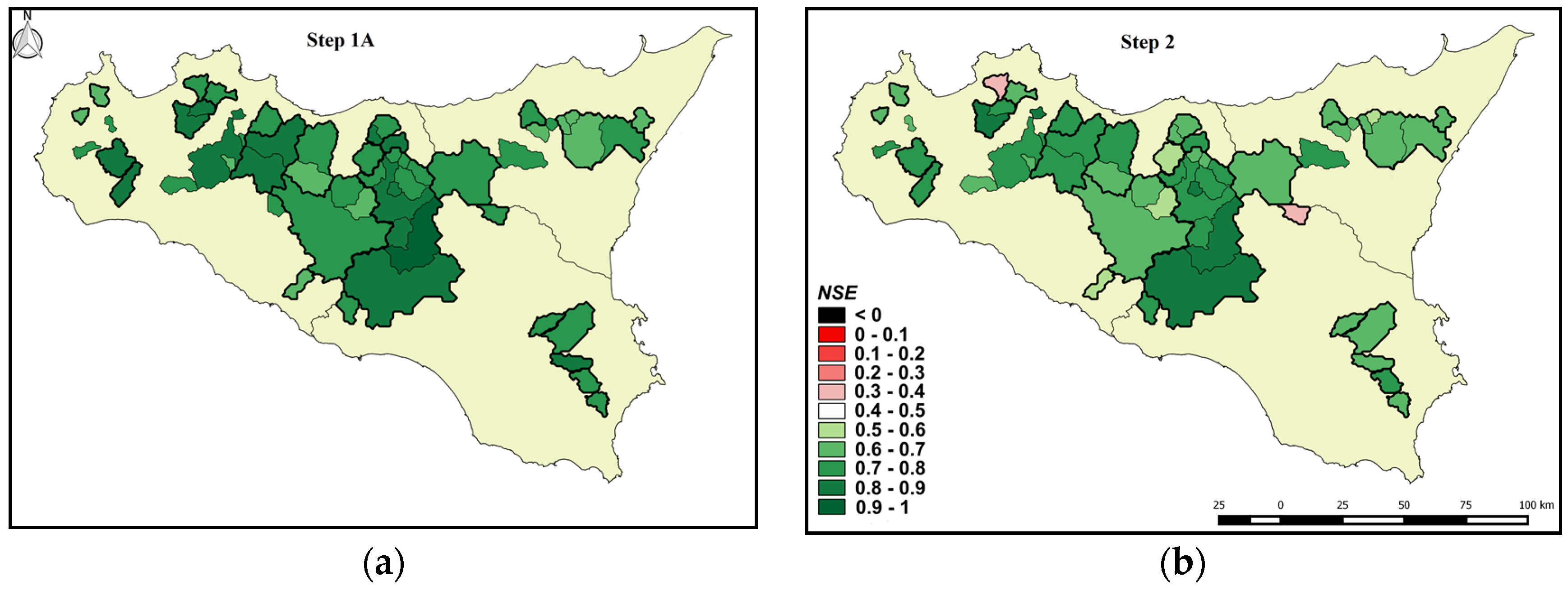
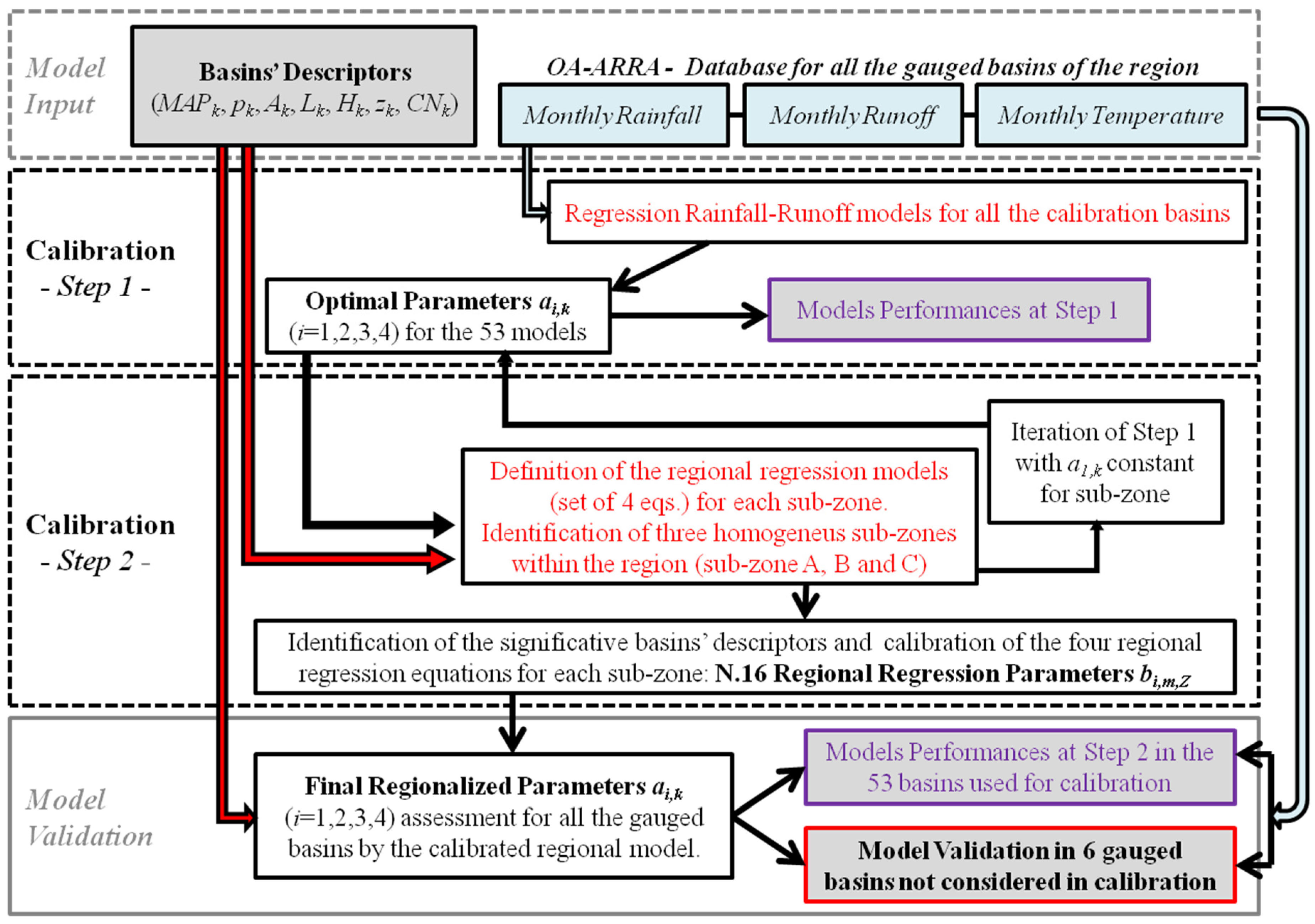
The model in Equation (1), with the four parameters individually calibrated for each site (Step 1A, Figure 6), has shown, over the 53 calibration basins, a high capacity for reproducing observed streamflows, with 
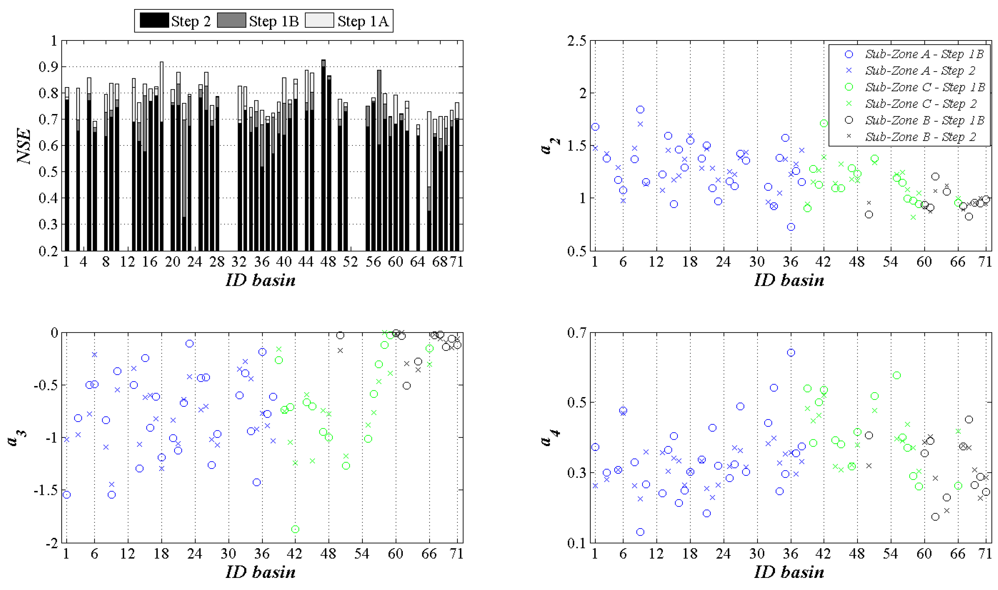
NSE values ranging from 0.64 to 0.93 and a mean of 0.77 (Table 4a). The 
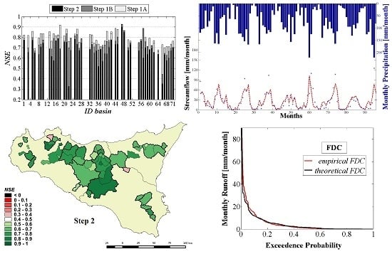
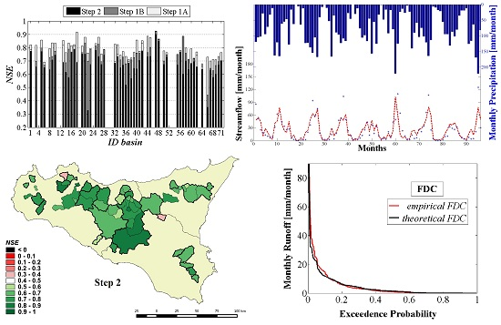
NSE values for such basins are represented in the histogram of Figure 7 (upper-left panel) and in the map of Figure 8a. From the latter as well as the results synthesized in Table 4a, it can be observed that the model in sub-zone C provides, on average, higher performance than results in the other two sub-zones.
The assumption that a1 is constant for each sub-zone has provided new sets of optimal values for a2,k, a3,k, and a4,k (Step 1B) whose corresponding performance, in terms of NSE, is reported in the same histogram of Figure 7 and Table 4a. The results are quite similar to those previously discussed (Step 1A), denoting a not significant decrease in the model’s performances; on average, a reduction in the order of 2% for the NSE indexes can be noticed. A significant NSE reduction (from 0.73 to 0.44) has been detected only for the ID 66 basin (sub-zone C), which is characterized by the lowest value of MAP and the second highest value of p.
As expected, the use of the regional relationships in Equation (4) for the ai,k parameter assessment (Step 2), reduces model performance with respect to the adoption of optimal (Steps 1A and B) parameter sets (histogram of Figure 7). Actually, this performance reduction is a price that has to be paid in order to provide a procedure able to assess runoff at ungauged sites. Nevertheless, the final model performances (after the Step 2) (Table 4a) remain in the range of acceptable values in terms of NSE, i.e., performance equal or more than satisfactory, according to the performance rating of Moriasi et al. [60], for all the calibration basins; the only two exceptions are the abovementioned ID 66 basin (sub-zone C), which had the lowest starting NSE value (i.e., NSE = 0.44 at Step 1B), and ID 22 basin (sub-zone A), where the resulting values are, however, positive and equal to 0.33 and 0.35, respectively. For this last basin, model performance reduction after the regionalization procedure is rather consistent, since, after Step 1B, the NSE was quite high (0.77). This could be attributable to the fact that the parameter values derived for this basin after Step 2 are markedly different from the corresponding values obtained at Step 1B, especially with regard to the parameter a4, whose regionalized value results were halved with respect to the previously obtained optimal value (from 0.43 to 0.23).
The percent reduction of the NSE after the regionalization, with respect to the NSE computed at the Step 1B, ranges from 0.17% to 57%, with the mean NSE (=0.69) over all the calibration basins reduced by almost 9% and denoting overall good performances. The efficiency reductions after the regionalization with respect to Step 1A are slightly more marked, with NSE reduced by 11% on average. This comparison is also emphasized in Figure 8, where the NSE obtained with the regionalized parameters (Figure 8b) and with the parameter sets of Step 1A (Figure 8a) are represented by the same color bar. Also, after the regionalized procedure, the model exhibits, on average, a higher accuracy for the basins in sub-zone C, with a mean NSE of 0.70 (Table 4a). The ID 47 basin (sub-zone C) has shown the highest NSE at every calibration phase (Table 4a), with a performance reduction after the regionalization (Step 2) equal to about 3%.
Model performances at Step 2 have also been assessed using three further statistical criteria measuring the agreement between observed and simulated monthly streamflow series: the mean error, ME (in mm/month); the dimensionless mean error, ME/ Q ¯ e m p , given by the ratio between the ME and the average observed streamflow ( Q ¯ e m p ); and the root mean square error, RMSE (in mm/month). For each index, the mean, the standard deviation, the minimum, the maximum, and the best values over all the calibration basins are synthesized in Table 4b. The results of this analysis have confirmed the outcomes relative to the performance index used for calibration (i.e., NSE), confirming the validity of the adopted calibration procedure. The model has globally provided a satisfying accuracy in terms of all the analyzed indexes and can be considered unbiased, as demonstrated by the relatively low values of ME. The values of ME, in absolute value, are lower than 3 mm/month for about 80% of the analyzed basins, while the mean ME/ Q ¯ e m p over the calibration basins is almost null. In terms of RMSE, the indexes have been of the same order of magnitude as those found through a similar modeling approach by Cutore et al. [47] for the Simeto river sub-basins (Sicily, Italy), with the worst performance (about 45 mm/month) obtained at basins ID 61, 67, and 68, which are all basins corresponding to NSE values lower than the mean value (0.69, 0.63, and 0.58, respectively).
The basin with the highest NSE (i.e., ID 47) also provided satisfactory performance in terms of ME, ME/ Q ¯ e m p , and RMSE (0.428, 0.042, and 5.05 mm/month, respectively). The basins with the lowest NSE (i.e., ID 22 and 66), showed the worst performance with respect to the other considered statistical criteria (ME = −6.67 and −2.54 mm/month, ME/ Q ¯ e m p = −0.49 and −0.69, RMSE = 15.37 and 9.97 mm/month, respectively). Only one basin (ID 40; sub-zone C) associated with a satisfying NSE (0.63), even if it was below the mean of the other basins, has provided relevant values for ME (11 mm/month) and ME/ Q ¯ e m p (0.35), denoting a weak performance that is, however, comparable to the worst performance obtained in different studies (e.g., [47]).
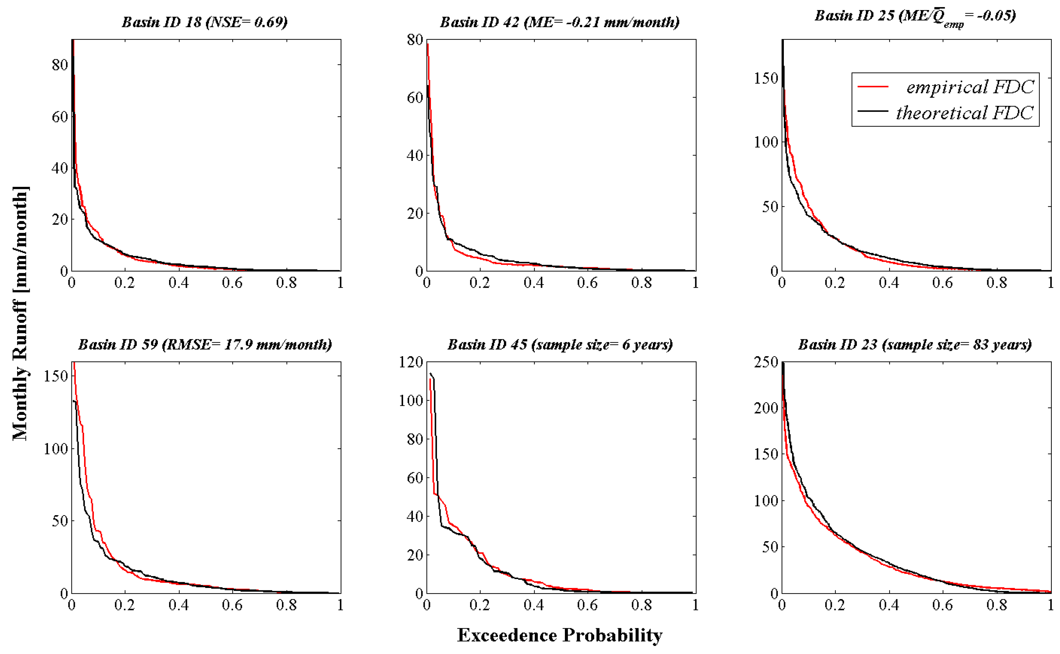
A comparison between monthly flow duration curves (FDCs) based on observed and simulated runoff values is reported in Figure 9 for different representative basins. Four examples, referring to basins with performance indexes approximately equal to the averages over all the calibration basins, are reported: basin ID 18 can be considered representative of basins with mean NSE, basin ID 42 is representative of basins with mean ME, basin ID 25 is representative of basins with mean ME/ Q ¯ e m p , while basin ID 59 is representative of basins with mean RMSE. Moreover, since the FDCs typically depend on the period considered, a comparison of the basins with the shortest (ID 45) and the longest (ID 23) sample size is also reported. Although some important details of the variations in flows can be obscured when the FDCs are computed using monthly data, rather than daily or finer resolution data, this analysis has been useful in confirming model accuracy. For all the examined basins, in fact, the model has satisfactorily reproduced the magnitudes associated with the various observed monthly runoff values, from the lowest and more frequent values to the highest and rarer ones, proving to be effective also in the assessment of the probability that a certain runoff value will be equaled or exceeded.

3.2. Model Validation

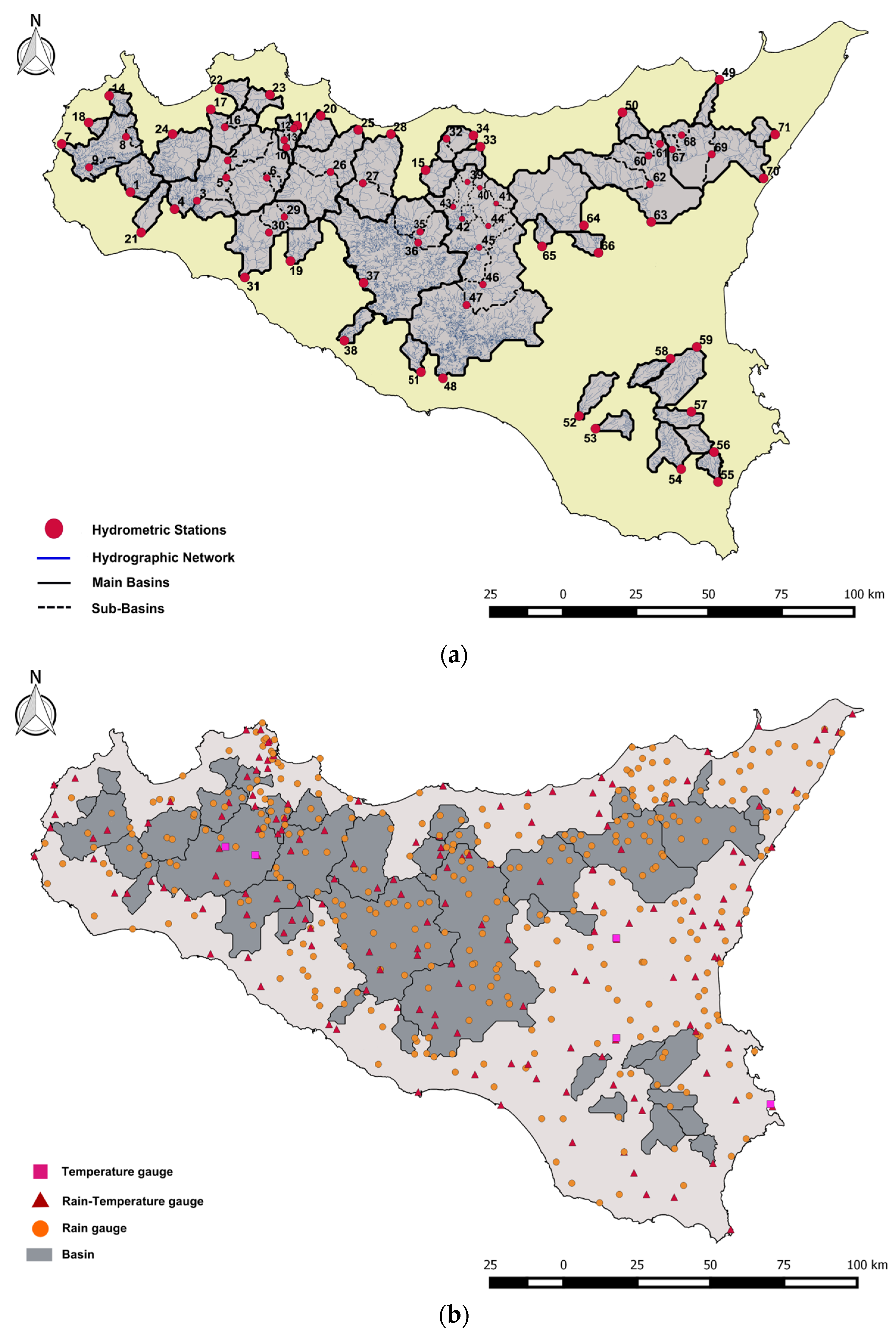
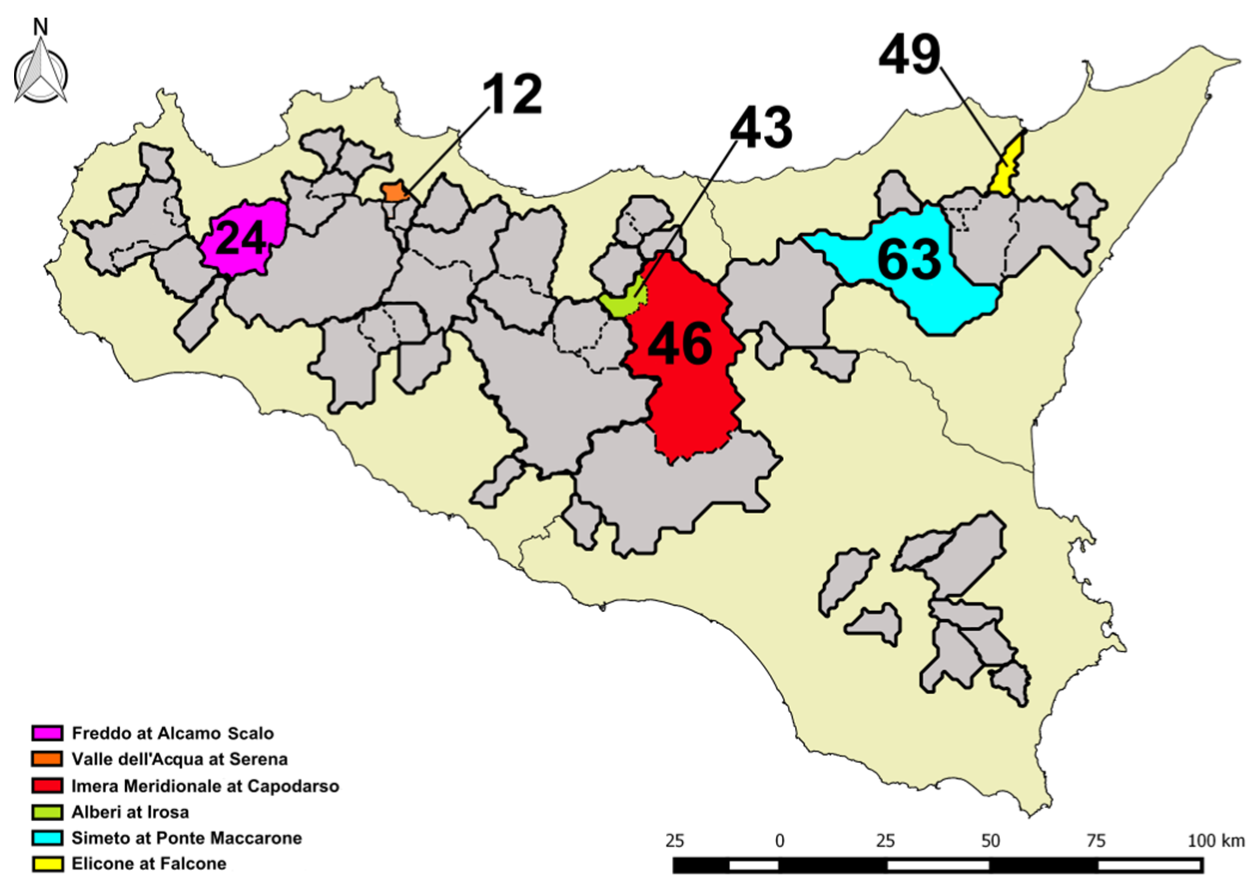
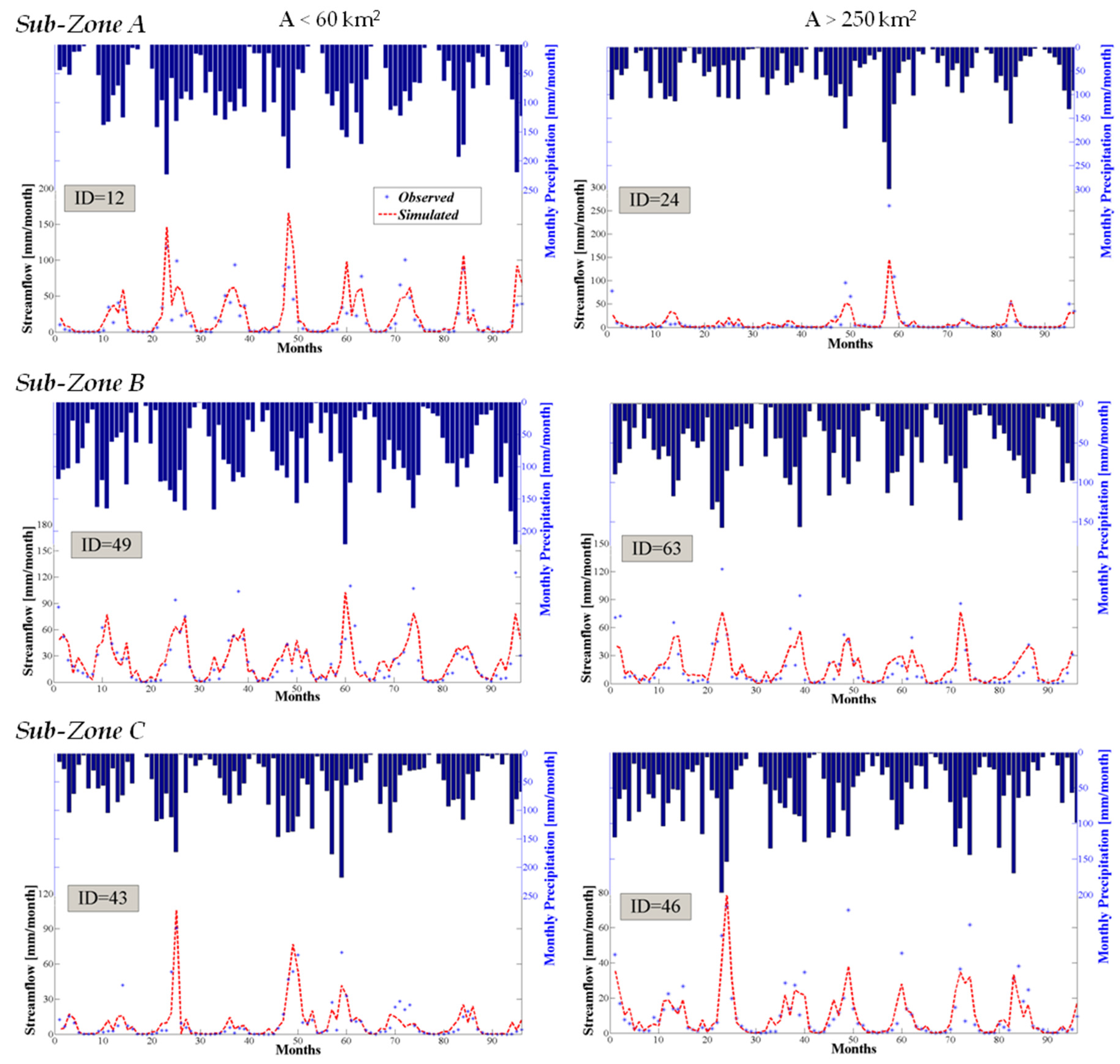
Model validation has been carried out by applying the model to the six validation basins (i.e., ID = 12, 24, 43, 46, 49, and 63; Figure 4) previously selected and not considered during the calibration (two of different area for each sub-zone). For each of them, the entire available historical monthly streamflow series has been reproduced by the model and compared with the corresponding empirical series, analyzing model performances through the same indexes previously used.
Performance achieved in the validation phase, summarized in Table 5, was similar among the different basins and very close to that measured at the calibration basins, with high NSE values (mean NSE = 0.74) and low ME, ME/ Q ¯ e m p and RMSE for all the six basins. Model series reproduction in the larger basins (ID 24, 63 and 46) was slightly more accurate (mean NSE = 0.79) than in the smaller ones (mean NSE = 0.71), but no significant difference can be noticed among model performances in validation over the different sub-zones. The results indicate the best performances (i.e., best NSE and RMSE) at the ID 46 basin (sub-zone C), with a sample size of 10 years, while the lowest performance was at the rainiest basins (ID = 12 and 49), characterized by the longest series (39 and 18 years, respectively).
Despite the fact that the validation basins are characterized by marked differences in terms of rainfall–runoff transformation, with mean annual runoff coefficients ranging from 0.14 (ID 43) to 0.34 (ID 49), the model has shown, over the six basins, an equal ability to capture the different basins’ hydrological response, with performance that can be classified as “good” in all the basins and, for two cases (i.e., basins ID 24 and 46), even as “very good” (i.e., NSE > 0.75).
Figure 10 depicts a comparison between observed and simulated monthly specific streamflow series (mm/month) for the six validation basins, also reporting the corresponding precipitation series. Simulated series are quite close to the observed series, reproducing well most of the peaks and null values. Despite the marked differences, in terms of both observed rainfall and streamflow, that can be noticed among the basins, the model captures rather accurately the monthly streamflow variability for both the smaller (left panels) and larger (right panels) basins in the three sub-zones. For example, the ID 12 basin is characterized by a seasonal streamflow regime, with about five months per year almost dry and frequent winter peaks with streamflow of about 100 mm/month, while the ID 24 basin is characterized by more regular behavior in the observed streamflow, with, on average, less rainfall and streamflow, and with only five months out of eight years having streamflow on the order of 100 mm/month; for both basins the model showed similar performance.

3.3. Model Performances at Different Aggregated Time Scales

Model performances have been further evaluated at different temporal aggregations, also considering the seasonal and the annual time scales. This analysis has been performed with regard to both the 53 calibration basins and the six validation basins, considered as a unique sample. More specifically, simulated monthly streamflow has been aggregated at the annual scale and also at the seasonal scale, considering the year as divided into two seasons: dry season, from April to September, and wet season, the remaining six months of the year.
Figure 11 compares all the estimates of the monthly, annual, and seasonal streamflow obtained from the regional model for all the basins with the corresponding observed streamflow. In the top left panel of the figure, a total of 12,312 theoretical monthly streamflow estimates are plotted against the corresponding empirical values, while the other scatter diagrams on the top refer to the annual streamflow values (middle panel, 1026 values) and the mean annual totals of streamflow for each basin (right panel, 59 values). In the bottom panels of Figure 11, the empirical and theoretical dry season (left panel), wet season (middle panel) streamflow values and the mean seasonal totals of streamflow for each basin (right panel) are similarly compared.
The high predictive ability of the model at the different aggregation scales is demonstrated by the fact that, for all the plots, most of the points are rather close to the perfect agreement lines (also reported in all the graphs), with high values of the coefficient of determination R2. These values are greater than 0.92 at the monthly level and 0.90 at the annual level. At the seasonal level, the model reproduces the dry season streamflow with an R2 of 0.95 and the wet season values with an R2 of 0.90. Although the cloud of points appears to be more disperse than in the other plots, the high value of R2 obtained at the monthly scale can be explained by the presence of a considerable number of observed values that are identically reproduced by the model (i.e., 22% of the null values and about 5% of the not-null streamflow).
Satisfying model performance has also been obtained with regard to the reproduction of the mean annual and seasonal totals of streamflow for the different basins (right panels of Figure 11), as is demonstrated by the resulting high R2 values (i.e., 0.95, 0.89, and 0.92 for the dry season, the wet season, and the annual analysis, respectively) and the low mean percent errors (from 2.2% for the annual and the wet season, to 12.5% for the dry season). The best performance in terms of absolute error (AE) was obtained at the basins with ID 42 for the dry season (AE = 0.21 mm/season), ID 37 for the wet season (AE = 0.02 mm/season), and ID 45 for the annual analysis (AE = 0.34 mm/season), while the worst resulted at basins with ID 56 for the dry season (AE = 65 mm/season), and ID 40 for the other two aggregation periods (AE = 121 mm/season and 135 mm/year for the wet season and the year, respectively). These values are consistent with results previously obtained at the monthly scale, where the ID 40 basin showed the worst performance in terms of both ME and ME/ Q ¯ e m p (Table 4b).
The results represented in Figure 11 have, therefore, demonstrated an elevated model capacity to reproduce not only the runoff at the monthly scale but also at coarser time resolutions, showing a satisfying ability to also reproduce the seasonal and interannual variability. A noteworthy aspect is that, despite the use of different models for the three subzones (i.e., same model structure and different regression parameters for each) and the application under 59 different boundary conditions (i.e., 59 different basins), all the estimates, at all the analyzed aggregation time scales, have shown comparable error, as can be observed from the left and middle panels of Figure 11.
Also at coarser time resolutions, model performances in validation basins have results comparable with those relative to the calibration basins, with similar residual errors. The analysis at the annual time scale for the validation basins has been further deepened by comparing simulated and observed annual streamflow series and computing all the different performance indexes previously used at the monthly scale. The results of this analysis, together with a comparison between empirical and theoretical values for the main annual statistics (mean, standard deviation, minimum, and maximum), are synthesized in Table 6.
For most of the cases, all the simulated main annual statistics are very close to the observed ones; moreover, it can be noticed that the reproduced variability is essentially never higher than that observed. The annual performance indexes show a good agreement between simulated and observed annual streamflow series: the highest NSE (0.96) was reached for the ID 43 basin, while the NSE values for the other basins are all higher than 0.64, with the only exception being the ID 46 basin, where a relatively low efficiency (NSE = 0.26) was obtained due to a low variance of the observed series that could negatively affect the NSE representativeness (see Equation (3)). Other indexes, in fact, denote good model performance at the ID 46 basin, while the ID 12 basin had the lowest performance, with values for ME and ME/ Q ¯ e m p slightly outside the ranges obtained for the other basins and also a relatively high value for RMSE.

4. Conclusions

This study applies a regional regressive model for the reconstruction of natural runoff series at the monthly or coarser time resolutions, intensively analyzing its performance. The importance of developing appropriate and easily transferable rainfall–runoff models able to reproduce reliable and long runoff series from climatic data is related to the fact that, in many practical cases, a runoff dataset is not available or insufficient in size, while long data series of climatic variables are much more often available, and, then, can be exploited to fill gaps in runoff records. A practical means of estimating natural runoff dynamics at ungauged stream sections or for rivers subject to regulation is fundamental for a variety of modern hydrological applications that involve a number of sectors (e.g., engineering, economic, environmental, etc.).
The idea proposed in this paper is to implement a calibration procedure for rainfall–runoff models based on the knowledge of “soft” basins information, usually available, such as rainfall, temperature, morphology, or land use. The model has been calibrated, through a simple two-step procedure, for the island of Sicily using a considerable number of basins and it has been validated in six basins representative of different basin sizes and different climatic subareas within the examined region.
This application may be considered as a benchmark for similar hydrological and climatic areas. Through a detailed description of the adopted methodology, some practical aspects that may be of interest for the model’s application to other regions have been explored. For instance, in this study, model performance has been revealed to be higher if the region is considered as divided into three different sub-zones. Moreover, six different basin attributes have been demonstrated to be functional in the definition of opportune regional equations for the estimation of the rainfall–runoff model parameters. The same methodology, applied to arid and semi-arid regions different from the study area of this work, could converge towards a different subdivision of the area of interest and/or different regional equations, characterized by different basin descriptors; nevertheless, the adopted structure for the rainfall–runoff models, which has shown extremely high accuracy at all Sicilian basins before the regionalization step, is expected to be equally valid. On the contrary, the application to humid regions should also encompass a redefinition of a more suitable conceptual scheme for the regression model, even if the proposed methodological approach could equally be followed.
For all the basins analyzed in this study, the regionalized model has shown satisfying accuracy, measured by different performance indexes, in reproducing the observed runoff at different time scales from monthly to aggregated seasonal and annual scales. Considering the Nash–Sutcliffe Efficiency (NSE) for the monthly series reproduction, it was rather weak for only two cases, but nevertheless positive (>0.33), denoting a “behavioral” modeling, while the NSE indexes for the other basins were all over 0.50, with “satisfactory” performance for 21% of cases, “good” for 53%, and “very good” for the remaining 26%, according to the performance criteria given by Moriasi et al. [60]. At coarser time resolutions, model performance did not show significant variations, with a very low percentage of error in the reproduction of both the seasonal and the annual mean runoff in any basin and an ability to also capture the seasonal and interannual runoff variability. The robustness of the model is strongly confirmed by the results in validation, in which a model reproduction of the historical runoff series at all the tested time scales gave results comparable to those obtained in calibration.
The obtained results have demonstrated how the model discussed in this study can be seen as a prompt and suitable option for the estimation of natural runoff time series at ungauged sites. It is worth emphasizing that an important application of the model is currently under development. In particular, a specific plug-in is being implemented within open-source GIS software (i.e., Quantum GIS 2.10) with the aim of automatizing data retrieval and processing procedures. After a preliminary preparation of an opportune Database Management System (DBMS) supporting the plug-in, the regional model, entirely re-coded in Python scripting language, will be able to rapidly assess natural runoff series (at monthly or higher time scales) for any basin of Sicily and any desired time window, both selected by an opportunely implemented Graphical User Interface (GUI). The plug-in will be based on a Data Processing Module (DPM), which, using spatial analysis techniques, will first proceed with the watershed classification (i.e., into sub-zones) and delineation, derivation of the monthly time series of mean areal precipitation and temperature, extraction of the six basin descriptors needed for the model and, then, derivation of the monthly runoff time series.

Acknowledgments

This work was partially funded by Messaggeri della Conoscenza, project title: “Ecoidrologia degli ecosistemi Mediterranei”, ID 177, funded by the Italian Ministry of Education, University, and Research.

Author Contributions

Dario Pumo is the first and corresponding author. All the authors (Dario Pumo, Francesco Viola, and Leonardo Valerio Noto) have relevantly contributed to this work, with different and equally important contributions to the design of the work, the acquisition, the analysis and the interpretation of data, the drafting, and the revising of the work.

Conflicts of Interest

The authors declare no conflict of interest.

Abbreviations

The following abbreviations are used in this manuscript:
OA-ARRAOsservatorio delle Acque-Agenzia Regionale per i Rifiuti e le Acque
SISIItaly’s Soil Information System
SCSSoil Conservation Service
GISGeographic Information System
DEMDigital Elevation Model
PAIPiano di Assetto Idrogeologico
NSENash-Sutcliffe Efficiency
FDCFlow Duration Curve
DBMSDatabase Management System
GUIGraphical User Interface
DPMData Processing Module

References

  1. Sivapalan, M.; Savenije, H.H.G.; Bloschl, G. Socio-hydrology: A new science of people and water. Hydrol. Process. 2012, 26, 1270–1276. [Google Scholar] [CrossRef]
  2. Sivapalan, M. Debates-Perspectives on socio-hydrology: Changing water systems and the “tyranny of small problems”—Sociohydrology. Water Resour. Res. 2015, 51, 4795–4805. [Google Scholar] [CrossRef]
  3. Gippel, C.J.; Bond, N.R.; James, C.; Xiquin, W. An asset-based, holistic, environmental flow assessment approach. Int. J. Water Resour. Dev. 2009, 25, 301–330. [Google Scholar] [CrossRef]
  4. Kendy, E.; Apse, C.; Blann, K. A Practical Guide to Environmental Flows for Policy and Planning with Nine Case Studies in the United States; The Nature Conservancy: Arlington County, VA, USA, 2012; Volume 74. [Google Scholar]
  5. Solans, M.A.; Mellado-Díaz, A. A Landscape-Based Regionalization of Natural Flow Regimes in the Ebro River Basin and Its Biological Validation. River Res. Appl. 2015, 31, 457–469. [Google Scholar] [CrossRef]
  6. Yin, X.A.; Petts, G.E.; Yang, Z.F. Ecofriendly River Management under Ever-Increasing Environmental Pressures. River Res. Appl. 2015, 31, 403–405. [Google Scholar] [CrossRef]
  7. Bourdin, D.R.; Fleming, S.W.; Stull, R.B. Streamflow modelling: A primer on applications, approaches and challenges. Atmos. Ocean 2012, 50, 507–536. [Google Scholar] [CrossRef]
  8. McMillan, H.; Freer, J.; Pappenberger, F.; Krueger, T.; Clark, M. Impacts of uncertain river flow data on rainfall-runoff model calibration and discharge predictions. Hydrol. Process. 2010, 24, 1270–1284. [Google Scholar] [CrossRef]
  9. Renard, B.; Kavetski, D.; Kuczera, G.; Thyer, M.; Franks, S.W. Understanding predictive uncertainty in hydrologic modeling: The challenge of identifying input and structural errors. Water Resour. Res. 2010, 46, W05521. [Google Scholar] [CrossRef]
  10. Del Giudice, D.; Reichert, P.; Bareš, V.; Albert, C.; Rieckermann, J. Model bias and complexity—Understanding the effects of structural deficits and input errors on runoff predictions. Environ. Model. Softw. 2015, 64, 205–214. [Google Scholar] [CrossRef]
  11. Abbott, M.B.; Bathurst, J.C.; Cunge, J.A.; O’Connell, P.E.; Rasmussen, J. An introduction to the European Hydrological System—Systeme Hydrologique European, ‘SHE’, 1: History and philosophy of a physically-based distributed modelling system. J. Hydrol. 1986, 87, 45–59. [Google Scholar] [CrossRef]
  12. Abbott, M.B.; Bathurst, J.C.; Cunge, J.A.; O’Connell, P.E.; Rasmussen, J. An introduction to the European Hydrological System—Systeme Hydrologique Europeen ‘SHE’. 2: Structure of a physically based, distributed modelling system. J. Hydrol. 1986, 87, 61–77. [Google Scholar] [CrossRef]
  13. Calver, A.; Wood, W.L. The Institute of Hydrology distributed model. In Computer Models of Watershed Hydrology; Singh, V.P., Ed.; Water Resources Publications: Littleton, CO, USA, 1995; pp. 595–626. [Google Scholar]
  14. Ivanov, V.Y.; Vivoni, E.R.; Bras, R.L.; Entekhabi, D. Catchment hydrologic response with a fully distributed triangulated irregular network model. Water Resour. Res. 2004, 40, W11102. [Google Scholar] [CrossRef]
  15. Noto, L.V.; Ivanov, V.Y.; Bras, R.L.; Vivoni, E.R. Effects of Initialization on Response of a Fully-Distributed Hydrologic Model. J. Hydrol. 2008, 352, 107–125. [Google Scholar] [CrossRef]
  16. Beven, K.; Freer, J. Equifinality, data assimilation, and uncertainty estimation in mechanistic modelling of complex environmental systems using the GLUE methodology. J. Hydrol. 2001, 249, 11–29. [Google Scholar] [CrossRef]
  17. Burnash, R.J.C. The NWS River Forecast System-catchment modeling. In Computer Models of Watershed Hydrology; Singh, V.P., Ed.; Water Resources Publications: Littleton, CO, USA, 1995; pp. 311–366. [Google Scholar]
  18. Boughton, W.C. The Australian water balance model. Environ. Model. Softw. 2004, 19, 943–956. [Google Scholar] [CrossRef]
  19. Chiew, F.H.S.; Peel, M.C.; Western, A.W. Application and testing of the simple rainfall-runoff model SYMHYD. In Mathematical Models of Small Watershed Hydrology and Applications; Singh, V.P., Frevert, D.K., Eds.; Water Resources Publications: Littleton, CO, USA, 2002; pp. 335–367. [Google Scholar]
  20. Jakeman, A.J.; Littlewood, I.G.; Whitehead, P.G. Computation of the instantaneous unit hydrograph and identifiable component flows with application to two small upland catchments. J. Hydrol. 1990, 117, 275–300. [Google Scholar] [CrossRef]
  21. Noto, L.V. Exploiting the Topographic Information in a PDM-Based Conceptual Hydrological Model. J. Hydrol. Eng. 2014, 19, 1173–1185. [Google Scholar] [CrossRef]
  22. Bergström, S. The HBV model. In Computer Models of Watershed Hydrology; Singh, V.P., Ed.; Water Resources Publications: Highlands Ranch, CO, USA, 1995; pp. 443–476. [Google Scholar]
  23. Oudin, L.; Andreassian, V.; Perrin, C.; Michel, C.; Le Moine, N. Spatial proximity, physical similarity, regression and ungaged catchments: A comparison of regionalization approaches based on 913 French catchments. Water Resour. Res. 2008, 44, W03413. [Google Scholar] [CrossRef]
  24. Arsenault, R.; Poissant, D.; Brissette, F. Parameter dimensionality reduction of a conceptual model for streamflow prediction in ungauged basins. Adv. Water Resour. 2015, 85, 27–44. [Google Scholar] [CrossRef]
  25. He, Y.; Bárdossy, A.; Zehe, E. A review of regionalisation for continuous streamflow simulation. Hydrol. Earth Syst. Sci. 2011, 15, 3539–3553. [Google Scholar] [CrossRef] [Green Version]
  26. Kizza, M.; Guerrero, J.L.; Rodhe, A.; Xu, C.-Y.; Ntale, H.K. Modelling catchment inflows into Lake Victoria: Regionalisation of the parameters of a conceptual water balance model. Hydrol. Res. 2013, 44, 789–808. [Google Scholar] [CrossRef]
  27. Parajka, J.; Viglione, A.; Rogger, M.; Salinas, J.L.; Sivapalan, M.; Blöschl, G. Comparative assessment of predictions in ungauged basins-Part 1: Runoff-hydrograph studies. Hydrol. Earth Syst. Sci. 2013, 17, 1783–1795. [Google Scholar] [CrossRef]
  28. Razavi, T.; Coulibaly, P. Streamflow prediction in ungauged basins: Review of regionalization methods. J. Hydrol. Eng. 2013, 18, 958–975. [Google Scholar] [CrossRef]
  29. Klemes, V. Operational testing of hydrological simulation models. Hydrol. Sci. J. 1986, 3, 13–24. [Google Scholar] [CrossRef]
  30. Vandewiele, G.L.; Elias, A. Monthly water balance of ungauged catchments obtained by geographical regionalisation. J. Hydrol. 1995, 170, 277–291. [Google Scholar] [CrossRef]
  31. Xu, C.Y.; Singh, V.P. A review on monthly water balance models for water resources investigation and climatical impact assessment. Water Resour. Manag. 1998, 12, 31–50. [Google Scholar]
  32. Guo, S.; Wang, J.; Yang, J. A semi-distributed hydrological model and its application in a macroscale basin in China. In Soil-Vegetation-Atmosphere Transfer Schemes and Large-Scale Hydrological Models; No. 270; IAHS Publishing: Wallingford, UK, 2001; pp. 167–174. [Google Scholar]
  33. Skøien, J.O.; Merz, R.; Bloschl, G. Top-kriging—Geostatistics on stream networks. Hydrol. Earth Syst. Sci. 2006, 10, 277–287. [Google Scholar] [CrossRef]
  34. Vandewiele, G.L.; Xu, C.Y.; Huybrecht, W. Regionalisation of physically-based water balance models in Belgium: Application to ungauged catchments. Water Resour. Manag. 1991, 5, 199–208. [Google Scholar] [CrossRef]
  35. McIntyre, N.; Lee, H.; Wheater, H.; Young, A.; Wagener, T. Ensemble predictions of runoff in ungauged catchments. Water Resour. Res. 2005, 41, W12434. [Google Scholar] [CrossRef]
  36. Ando, Y. Regionalization of parameters using basin geology, land use and soil type in a storm rainfall-runoff relationship. In Regionalization in Hydrology; Beran, M.A., Brilly, M., Becker, A., Bonacci, O., Eds.; No. 191; IAHS Publishing: Wallingford, UK, 1990; pp. 211–218. [Google Scholar]
  37. Bergmann, H.; Richtig, G.; Sackl, B. A distributed model describing the interaction between flood hydrographsand basin parameters. In Regionalization in Hydrology; Beran, M.A., Brilly, M., Becker, A., Bonacci, O., Eds.; No. 191; IAHS Publishing: Wallingford, UK, 1990; pp. 91–102. [Google Scholar]
  38. Post, D.A.; Jakeman, A.J. Relationships between catchment attributes and hydrological response characteristics in small Australian mountain ash catchments. Hydrol. Process. 1996, 10, 877–892. [Google Scholar] [CrossRef]
  39. Boughton, W.; Chiew, F. Estimating runoff in ungauged catchments from rainfall, PET and the AWBM model. Environ. Model. Softw. 2007, 22, 476–487. [Google Scholar] [CrossRef]
  40. Deckers, D.L.E.H.; Booij, M.J.; Rientjes, T.H.M.; Krol, M.S. Catchment Variability and Parameter Estimation in Multi-Objective Regionalisation of a Rainfall-Runoff Model. Water Resour. Manag. 2010, 24, 3961–3985. [Google Scholar] [CrossRef]
  41. Pumo, D.; Noto, L.V.; Viola, F. Ecohydrological modelling of flow duration curve in Mediterranean river basins. Adv. Water Resour. 2013, 52, 314–327. [Google Scholar] [CrossRef]
  42. Pruski, F.F.; Nunes, A.D.A.; Pruski, P.L.; Rodriguez, R.D.G. Improved regionalization of streamflow by use of the streamflow equivalent of precipitation as an explanatory variable. J. Hydrol. 2013, 476, 52–71. [Google Scholar] [CrossRef]
  43. Viola, F.; Pumo, D.; Noto, L.V. EHSM: A conceptual ecohydrological model for daily streamflow simulation. Hydrol. Process. 2013, 28, 3361–3372. [Google Scholar] [CrossRef]
  44. Kim, H.S.; Lee, S. Assessment of the adequacy of the regional relationships between catchment attributes and catchment response dynamics, calibrated by a multi-objective approach. Hydrol. Process. 2014, 28, 4023–4041. [Google Scholar] [CrossRef]
  45. Pumo, D.; Viola, F.; La Loggia, G.; Noto, L.V. Annual flow duration curves assessment in ephemeral small basins. J. Hydrol. 2014, 519, 258–270. [Google Scholar] [CrossRef]
  46. Hawley, M.E.; McCuen, R.H. Water yield estimation in western United States. J. Irrig. Drain. Div. 1982, 108, 25–35. [Google Scholar]
  47. Cutore, P.; Cristaudo, G.; Campisano, A.; Modica, C.; Cancelliere, A.; Rossi, G. Regional Models for the Estimation of Streamflow Series in Ungauged Basins. Water Resour. Manag. 2007, 21, 789–800. [Google Scholar] [CrossRef]
  48. Pumo, D.; Caracciolo, D.; Viola, F.; Noto, L.V. Climate change effects on the hydrological regime of small non-perennial river basins. Sci. Total Environ. 2016, 542, 76–92. [Google Scholar] [CrossRef] [PubMed]
  49. Di Piazza, A.; Lo Conti, F.; Noto, L.V.; Viola, F.; La Loggia, G. Comparative analysis of different techniques for spatial interpolation of rainfall data to create a serially complete monthly time series of precipitation for Sicily, Italy. Int. J. Appl. Earth Obs. Geoinf. 2011, 13, 396–408. [Google Scholar] [CrossRef]
  50. Di Piazza, A.; Lo Conti, F.; Viola, F.; Eccel, E.; Noto, L.V. Comparative Analysis of Spatial Interpolation Methods in the Mediterranean Area: Application to Temperature in Sicily. Water 2015, 7, 1866–1888. [Google Scholar] [CrossRef] [Green Version]
  51. Arsenault, R.; Brissette, F. Continuous streamflow prediction in ungauged basins: The effects of equifinality and parameter set selection on uncertainty in regionalization approaches. Water Resour. Res. 2014, 6135–6153. [Google Scholar] [CrossRef]
  52. De Jager, A.L. Preparing CORINE Land Cover Data for Use. Optimization of Land Cover Data Using a Database and a Topological GIS Platform; JRC-IES, JRC68174, EUR 25163 EN.; Publications Office of the European Union: Luxembourg, 2012; ISBN 978-92-79-22720-2. ISSN 1018-5593. [Google Scholar]
  53. Costantini, E.A.C.; Dazzi, C. The Soils of Italy. In World Soils Book Series; Springer: Dordrecht, The Netherlands, 2013; ISBN: 978-94-007-5641-0 (Print) 978-94-007-5642-7 (Online). [Google Scholar]
  54. Soil Conservation Service (SCS). Hydrology. In National Engineering Handbook; Soil Conservation Service, USDA: Washington, DC, USA, 1993; Section 4, Chapter 4. [Google Scholar]
  55. Viola, F.; Noto, L.V.; Cannarozzo, M.; La Loggia, G. Regional flow duration curve for ungauged sites in Sicily. Hydrol. Earth Syst. Sci. 2011, 15, 323–331. [Google Scholar] [CrossRef] [Green Version]
  56. Cannarozzo, M.; Noto, L.V.; Viola, F.; La Loggia, G. Annual runoff regional frequency analysis in Sicily. Phys. Chem. Earth 2009, 34, 679–687. [Google Scholar] [CrossRef]
  57. Cannarozzo, M.; D’Asaro, F.; Ferro, V. Regional rainfall and flood frequency analysis for Sicily using the two component extreme value distribution. Hydrol. Sci. J. 1995, 40, 19–42. [Google Scholar] [CrossRef]
  58. Gyawali, R.; Griffis, V.W.; Watkins, D.W.; Fennessey, N.M. Regional regression models for hydro-climate change impact assessment. Hydrol. Process. 2015, 29, 1972–1985. [Google Scholar] [CrossRef]
  59. Nash, J.E.; Sutcliffe, J.V. River flow forecasting through conceptual models, 1. A discussion of principles. J. Hydrol. 1970, 10, 282–290. [Google Scholar] [CrossRef]
  60. Moriasi, D.N.; Arnold, J.G.; Van Liew, M.W.; Bingner, R.L.; Harmel, R.D.; Veith, T.L. Model evaluation guidelines for systematic quantification of accuracy in watershed simulations. Trans. ASABE 2007, 50, 885–900. [Google Scholar] [CrossRef]
Figure 1. Study area (Sicily, Italy). (a) Location of the analyzed river basins with position of the relative hydrometric gauging stations. The hydrographic network is also highlighted; (b) Location and typology of the meteo-climatic stations.
Water 08 00209 g001
Figure 2. (a) Elevations (m a.s.l.) from the considered Digital Elevation Model (DEM) of Sicily; (b) spatial distribution of the CN parameter (raster map by Regione Sicilia).
Water 08 00209 g002
Figure 3. Homogeneous sub-zones (A, B, and C) for parameter regionalization.
Water 08 00209 g003
Figure 4. The six validation basins.
Water 08 00209 g004
Figure 5. Schematic representation of the different phases of model calibration and validation.
Water 08 00209 g005
Figure 6. Optimal calibration parameters (a1, a2, a3, and a4) after Step 1A for all the calibration basins. Different markers are used for each sub-zone.
Water 08 00209 g006
Figure 7. Parameters and model performances at the different calibration phases: optimal calibration parameters (a2, a3, and a4) after Step 1B and regionalized parameters after Step 2 for all the calibration basins; in the upper-left histogram, the resulting NSE values after each calibration phase (Step 1A, Step 1B, and Step 2).
Water 08 00209 g007
Figure 8. Comparison between model performance (NSE) obtained at Step 1A (a) and Step 2 (b).
Water 08 00209 g008
Figure 9. Comparison between observed (red curves) and simulated (black curves) duration curves of monthly runoff for different calibration basins.
Water 08 00209 g009
Figure 10. Observed (marks) and simulated (dashed lines) monthly streamflow series (mm/month) for the validation basins, with histograms denoting the underlying precipitation series. Only the first eight years are reported. Upper panels refer to the basins of sub-zone A, middle panels to the basins in sub-zone B, while lower panels refer to sub-zone C. Left panels refer to the smaller basins (A < 60 km2), while right panels refer to the largest ones (A > 250 km2).
Water 08 00209 g010
Figure 11. Model performance at the monthly, seasonal, and annual scale for all the calibration and validation basins. In the right two panels, the empirical mean annual (top) and seasonal (bottom) streamflow totals for each basin are plotted against the corresponding theoretical values. Dry season is the six months from April to September, while the Wet season is the remaining part of the year. Dashed lines indicate the perfect agreement between observed and simulated values.
Water 08 00209 g011
Table 1. Watersheds and hydrometric gauge station names (St. Name); identification code (ID); typology (Type): main basin (MB) or sub-basin (SB) and sub-zone (A, B, or C); observation period: first and last year of observation and total sample size in years (yr).
IDSt. NameWatershedTypeObservationsIDSt. NameWatershedTypeObservations
fromtoyrfromtoyr
1PozzilloDeliaMBA195919782037PassofondutoPlataniMBA1956196611
2SparaciaBelice DestroSBA195519873338MandorletoS. BiagioMBA1976198611
3FinocchiaraSenoreSBA196119862639PetraliaImera Mer.SBC1986199712
4Ponte BeliceBeliceMBA195519942940RaffoSalsoSBC1979198911
5Case BalateBeliceSBA195519802641RegiovanniGangiSBC1982199615
6Piano ScalaCorleoneSBA19581963642CastelloCastelloSBC1983199715
7ChinisiaBirgiMBA197120012343IrosaAlberiSBC1992200110
8La ChineaFastaiaSBA196219983544MonzanaroSalsoSBC1985199713
9RinazzoChitarraSBA197219881745Cinque ArchiImera Mer.SBC198019856
10LupoEleuterioSBA193720065646CapodarsoImera Mer.SBC1963197210
11RisalaimiEleuterioMBA196119902847BeseroImera Mer.SBC195919668
12SerenaV. dell'AcquaSBA196120023948DrasiImera Mer.MBC1960197011
13RossellaEleuterioSBA193719571349FalconeEliconeMBB1976199618
14LentinaForgiaMBA197120022950Passo GalloRosmarinoMBB198819956
15ScillatoImera Sett.MBA197620032751DonnapaolaGibbesiMBC1971199215
16FellamonicaJatoSBA197320021852S. PietroFicuzzaMBC1974199417
17TaurroTaurroMBA195519671253MazzaronelloParà ParàMBC197719826
18SaponeBaiataMBA196820012754CastelluccioTellaroMBC1974199818
19CorvoMagazzoloMBA19721979655NotoAsinaroMBC1973199815
20MiliciaMiliciaMBA197620052456ManghisiCassibileMBC1984199913
21S.EliaModioneMBA19721981957S. NicolaAnapoMBC1972199827
22ZuccoNocellaMBA195820034258RappisTrigonaMBC1972198411
23ParcoOretoMBA192420068359ReinaZenaMBC1972198110
24Alcamo ScaloFreddoMBA197219871060PetrosinoMartelloSBB1981200118
25MonumentaleS. LeonardoMBA192819845561ChiusittaSaracenoSBB1982199816
26VicariS. LeonardoSBA192419872662SerravalleTroina di S.SBB1975200523
27RoccapalumbaTortoSBA198320042163MaccaroneSimetoMBB197519828
28Bivio CerdaTortoMBA196920001864GaglianoSalsoMBB1975200426
29San CarloSosioSBA198720021365Case CarellaCrisàMBC1958198625
30SosioSosioSBA193019421366TorricchiaSciaguanaMBC1969198916
31Poggio DianaPoggio DianaMBA19341939667ZarbataFlascioSBB1981200320
32Ponte GrandeIsnelloSBA198420001768S. GiacomoAlcantaraSBB1983200018
33GuglielmottoT. dei MuliniMBA199320031169MoioAlcantaraSBB1939200235
34Ponte VecchioCastelbuonoMBA198720031770AlcantaraAlcantaraMBB1934200132
35BruciatoBeliciSBA198119921271RanciaraForza d'AgròMBB198319937
36MarianopoliBeliciSBA199720026
Table 2. Basin descriptors: MAP = mean annual precipitation; p = seasonal precipitation index; A = drainage area; L = main river length; H = mean basin altitude; z = basin relief; CN = Curve Number.
IDMAPpALHzCNIDMAPpALHzCN
mm/yr-km2kmm a.s.lm-mm/yr-km2kmm a.s.lm-
16780.019138.620.9127261180.5376200.0261228.647.12519114079.5
27080.018127.832.8743794682.0386200.01265.614.8634444982.8
36620.01975.923.64407103679.5397600.03328.65.63122083875.9
46730.021813.965.47439139879.3407200.01720.63.72108387879.8
57170.021338.239.27569128978.7416700.01557.68.1085866080.6
69550.01019.47.65805108782.9427200.02622.64.7463325981.3
75140.020343.836.1219876780.0437200.03550.618.0074656180.3
85820.02723.97.1032746579.0446700.041185.618.68790121480.8
94750.01637.418.1215830879.8456300.011545.235.34730138580.2
107820.0259.75.92796107876.5465800.037658.650.52691143680.1
117930.02155.813.1063181576.3476000.0351003.659.57634149679.6
128280.02024.110.6565174574.7485300.0331887.692.18531166278.7
139610.0259.35.0665143078.1499070.04754.617.27696124971.2
145710.02050.123.8628790683.1506740.07373.610.691021133974.0
157410.023105.215.10837161275.7514940.03268.615.8832521283.4
168320.01852.614.92616108578.6525120.053101.619.5338439176.6
177860.017166.823.38418118078.7537610.01267.613.2946164771.6
184750.01629.111.5311127585.5545710.057138.617.9445653071.9
197570.033180.131.29531135279.0555680.03654.114.0436449474.8
206230.029112.617.3848191281.1567160.05368.614.5135551173.4
216220.02681.226.9425860980.2577040.04182.615.3362553869.4
229150.02461.614.72527108574.1585880.04671.414.9646760357.1
2310260.02170.411.36601120674.9596240.050227.627.9736488866.7
246230.021270.632.3224474181.2608830.04543.69.81132082465.0
256990.024498.050.73584145079.46111550.03518.65.05144538269.1
267040.016246.828.23676128380.2626710.051159.426.3296991479.2
275220.018173.380.0557064580.7636500.052693.652.321085278173.6
285370.017415.458.32503127680.4646500.042502.633.82791115080.2
296730.03188.119.37713123973.1656420.03250.69.9560755581.8
308990.018106.118.1686192577.6664290.05263.613.6041147378.1
318330.016391.852.90614138176.76710080.04317.64.50126850467.7
327950.03334.69.671229136869.76810340.02835.67.69125840268.5
338200.03361.610.771139151672.7698420.043306.626.371117261967.7
348000.036105.621.24893172673.8709190.031557.647.50912313269.4
356400.012134.616.2560666079.3719760.03454.68.87688101262.8
366200.031234.620.9260067579.8
Table 3. Regional regression parameters bi,j,Z for the estimation of the parameters ai,k by Equation (4).
Regional Regression Parameters for a1,k
sub-zone (Z)b1,Z
A0.20503
B0.24834
C0.24138
Regional Regression Parameters for a2,k
sub-zone (Z)b2,1,Zb2,2,Zb2,3,Zb2,4,Zb2,5,Z
A4.21951−0.00062−7.61813−0.00063−0.02503
B1.08348−0.00034−3.50405−0.000070.00567
C−0.166280.00106−6.65375−0.000600.01663
Regional Regression Parameters for a3,k
Sub-zone (Z)b3,1,Zb3,2,Zb3,3,Zb3,4,Zb3,5,Z
A−5.003500.001468.756650.000760.03254
B0.293980.000302.147310.00013−0.01299
C1.64497−0.0020021.687260.00140−0.03573
Regional Regression Parameters for a4,k
sub-zone (Z)b4,1,Zb4,2,Zb4,3,Zb4,4,Zb4,5,Z
A−1.13660−0.00002−0.000030.000330.01651
B0.28308−0.000180.0000040.00016−0.00164
C0.355550.00014−0.000270.000210.00119
Table 4. (a) Analysis of NSE indexes (mean for sub-zone, and mean, standard deviation, minimum, and maximum over all the calibration basins) at the different calibration stages (Step 1A, Step 1B, Step 2); (b) Analysis (mean, standard deviation, minimum, and maximum) of other performance indexes (ME = mean error; ME/ Q ¯ e m p = dimensionless mean error; RMSQ = root mean square error) over the calibration basins after the regionalization (Step 2). The basin ID codes corresponding to the best, minimum, and maximum performance indexes are also reported within brackets.
(a)Mean NSE for Sub-ZoneNSE (53 Calibration Basins)
Calibration StageABCMeanSt. Dev.Min (ID)Max (ID)
Step 1A0.780.710.800.770.0660.64 (68)0.93 (47)
Step 1B0.770.690.770.750.0800.44 (66)0.92 (47)
Step 20.690.650.700.690.1000.32 (22)0.90 (47)
(b) Step 2 (53 Calibration Basins)
Model Statistics MeanSt. Dev.Min (ID)Max (ID)Best (ID)
ME (mm/month) 0.283.74−8.32 (39)11.03 (40)0.113 (1)
ME/ Q ¯ e m p −0.020.21−0.69 (66)0.35 (40)0.009 (1)
RMSE (mm/month) 16.4610.003.74 (48)46.55 (61)3.74 (48)
Table 5. Model performances (NSE, ME, ME/ Q ¯ e m p , RMSQ) at the monthly scale for the validation basins. The identification number (ID), the sub-zone, the area (A), the simulated–observed series size in years (Size), and the observed mean annual precipitation (MAP) are also reported for each basin.
Validation BasinsMonthly Performance Indexes
IDSub-ZoneSizeAMAPNSEMEME/ Q ¯ e m p RMSE
(yr)(km2)(mm/yr)(mm/month)(mm/month)
12A3924.18280.70−5.01−0.3016.19
24A10270.66230.760.530.0514.44
49B1854.69070.710.380.0218.22
63B8693.66500.74−1.79−0.1111.67
43C1050.67200.73−0.83−0.117.85
46C10658.65800.790.300.036.95
Table 6. Model performances (NSE, ME, ME/ Q ¯ e m p , RMSQ) at the annual scale for the validation basins. The observed (Emp.) annual statistics (mean, standard deviation, minimum, and maximum) are also compared with the corresponding simulated (Theo.) values.
Validation Basins: Annual StatisticsAnnual Performance Indexes
IDSub-ZoneMeanSt. Dev.MinMaxNSEMEME/ Q ¯ e m p RMSE
(mm/yr)(mm/yr)(mm/yr)(mm/yr)(mm/yr)(mm/yr)
Emp.Theo.Emp.Theo.Emp.Theo.Emp.Theo.
12A20426312812917725556280.64−58.36−0.2975.53
24A12912320311322535863750.796.620.0586.54
49B306300135941641857485860.866.100.0249.62
63B18621787631081443493380.68−30.62−0.1645.70
43C98108918820513063200.96−9.98−0.1017.55
46C126121272992621581600.265.350.0421.90

