1. Introduction
A natural temporary imbalance of water availability, consisting of persistent lower-than-average or higher-than-average precipitation, can cause extreme dry and wet conditions that adversely impact agricultural yields, water resources, infrastructure and human systems. For example, dry conditions have severe consequences because they can give rise to agricultural yield losses and water shortages [
1,
2]. They also damage natural ecosystems [
3,
4] and forestry [
5,
6] and lead to soil degradation and desertification [
7,
8], social alarm [
9], famine and impoverishment [
10,
11]. Conversely, wet conditions can cause flood, damage crops, reduce yields, and contribute to groundwater contamination [
12,
13,
14,
15,
16,
17]. For these reasons, the analysis of the distribution of dry and wet periods has always been a concern for researchers [
18,
19,
20,
21,
22,
23,
24,
25,
26]. In general, climate anomalies are quantitatively assessed through indices that allow scientists to characterize them in terms of intensity, duration, frequency, recurrence probability and spatial extent [
27,
28]. Among the several indices, two of the most commonly used are the standardized precipitation index (SPI), which transforms monthly precipitation time series into a standardized normal distribution, and the drought severity index (DSI), which uses accumulated monthly precipitation anomalies. In particular, the SPI has found widespread application in different countries of the world [
29,
30,
31,
32,
33,
34,
35], in the Mediterranean basin [
36,
37,
38] and also in Central [
39] and Southern Italy [
40,
41,
42,
43,
44,
45,
46]. The SPI is easier to calculate than more complex indices because it is based on precipitation alone for estimating wet or dry conditions [
38,
47]. Moreover, these conditions can be monitored by the SPI on a variety of time scales from sub-seasonal to inter-annual scales [
43].
Generally, the probabilistic structure of dry and wet periods, especially with a long duration, cannot be properly investigated due to the limited number of events in the historical series [
48]. Moreover, complete data are strictly required to perform the analysis of wet and dry periods, because missing values may significantly influence estimates of event duration and the character of their alternation [
49]. In order to overcome such a difficulty, the probabilistic behavior of dry and wet periods characteristics can be derived analytically, assuming a given stochastic structure of the underlying hydrological and meteorological series [
24,
50,
51,
52,
53,
54,
55,
56,
57,
58,
59]. This has led to the development of stochastic models frequently used to produce long rainfall series that are statistically similar to historical records (e.g., [
60]). In particular, mathematical modeling of hydrological data as a stochastic process is of interest to a variety of hydrological areas such as flood forecasting, reservoir operations and agricultural planning [
61,
62,
63]. Current state-of-the-art stochastic precipitation models at a single site or for multiple sites can reproduce a wide range of statistics from hourly scale extremes to larger aggregation periods [
64,
65,
66,
67,
68,
69,
70,
71,
72,
73,
74,
75]. In particular, numerous approaches for the stochastic modeling of daily rainfall data are available in the hydrological and climatological literature [
76,
77,
78,
79,
80,
81,
82,
83,
84]. These models are widely used because they are easy to formulate and fast to implement [
26]. Stochastic modeling also allows for accounting of potentially wider range of conditions that may not be necessarily represented in poorly sampled data. Moreover, by means of stochastic simulators, effectively intrinsic variability, not associated with forced signals (e.g., by global warming), can be generated; this variability is important because it places uncertainties on projections. However, very little work has been done on stochastic generation of monthly rainfall data [
85] because in the past low attention was paid to totals at this time aggregation.
The aims of this study are:
- (a)
to propose a stochastic procedure for modeling precipitation at monthly scale;
- (b)
to analyze dry and wet periods through the application of the standardized precipitation index (SPI) to a set of monthly rainfall series generated by the proposed model through a Monte Carlo procedure. These results have been compared with the ones obtained through the application of the drought severity index (DSI).
In particular, the model has been applied to a set of monthly rainfall series observed in Southern Italy (the region of Calabria).
3. Case Study
The study area (the region of Calabria) is a peninsula with an oblong shape occupying the southern part of Italy. It has a surface of 15,080 km
2 and a coastline of 738 km on the Ionian and Tyrrhenian Seas. Calabria has a length of about 250 km and a width ranging between 31 and 111 km. The maximum elevation is 2267 m a.s.l., while the average elevation is 597 m a.s.l. [
100].
Because of its geographic position and mountainous nature, Calabria has a high climatic variability with a typically dry summer subtropical climate, also known as the Mediterranean climate [
101]. Its coastal zones are characterized by mild winters and hot summers with little precipitation. In particular, the Ionian side, which is influenced by currents coming from Africa, has high temperatures with short and heavy precipitation, while the Tyrrhenian side is influenced by western air currents and presents milder temperatures and considerable orographic precipitation. In the inland zones there are colder winters (with snow) and fresher summers (with some precipitation) than those marking the coastal zones [
102].
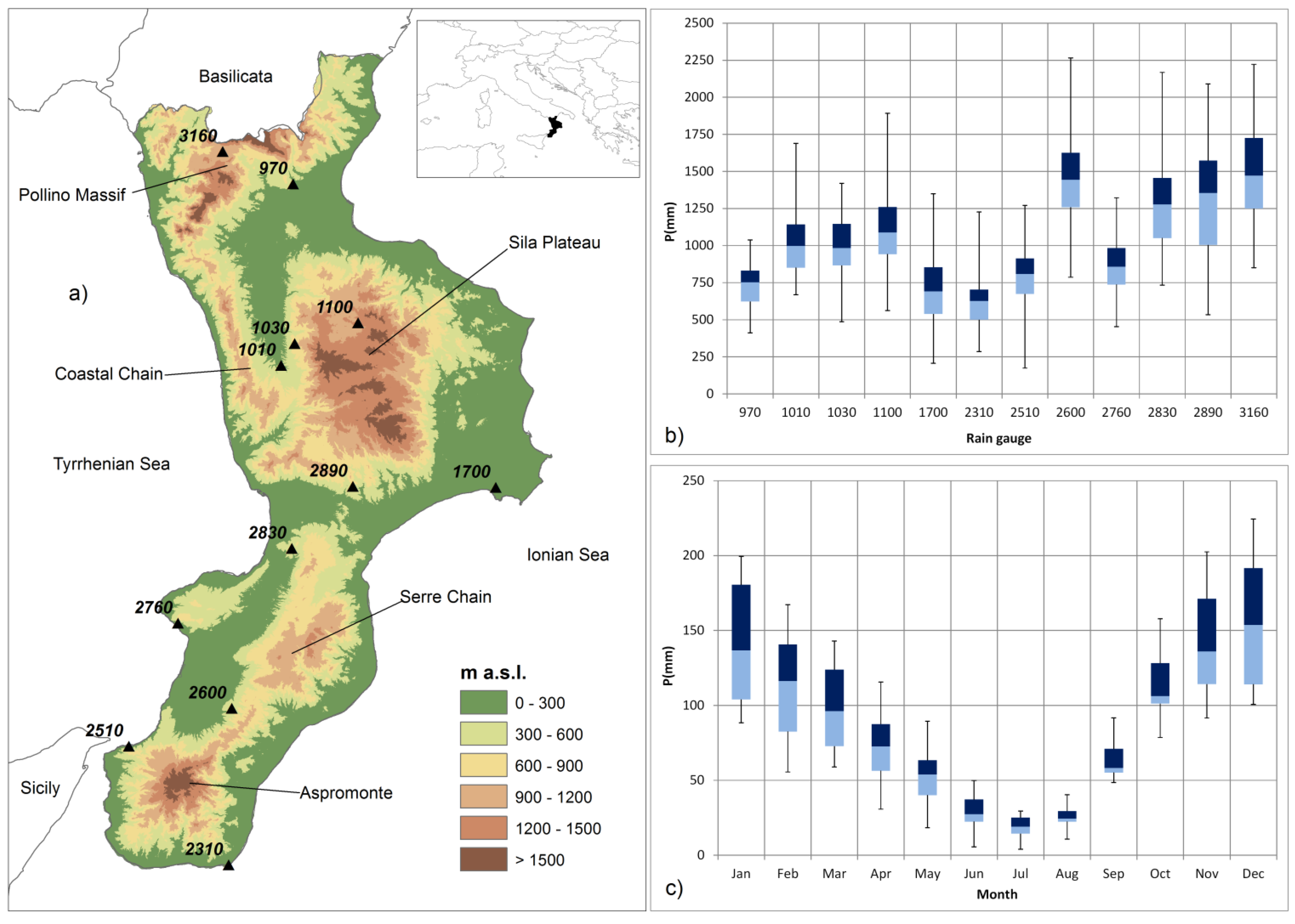
Monthly precipitation data have been collected and published in the region of Calabria by the former Italian Hydrographic Service. In this work, particular attention has been given to the problems arising from the low quality and inhomogeneities of the data series. Thus, the monthly database used in the further analysis was a part of the high-quality one presented in a previous study [
103], in which a multiple application of the Craddock test [
104] to detect the inhomogeneities was performed. In particular, in the present work, a set of 12 monthly total precipitation series, which were found to be homogeneous for the period 1916–2011, were selected. In
Figure 1, the study area and the characterization of the rainfall series through box plots are presented. The main features of the rain gauges are shown in
Table 2, together with the percentages of missing data. The percentage of gaps in the series ranges between 1.5 and 12.4%, and is mostly detected during the Second World War period.
Table 2.
Main features of the selected rain gauges.
Table 2.
Main features of the selected rain gauges.
| Code | Rain Gauge | Longitude (Degrees) | Latitude (Degrees) | Elevation (m a.s.l.) | First Year | Last Year | Missing Data (%) |
|---|
| 970 | Cassano allo Ionio | 16.319 | 39.783 | 250 | 1921 | 2011 | 10.4 |
| 1010 | Cosenza | 16.265 | 39.287 | 242 | 1916 | 2011 | 3.5 |
| 1030 | San Pietro in Guarano | 16.314 | 39.346 | 660 | 1922 | 2011 | 2.5 |
| 1100 | Cecita ex Acquacalda | 16.538 | 39.400 | 1180 | 1923 | 2011 | 7.1 |
| 1700 | Isola di Capo Rizzuto | 17.094 | 38.961 | 90 | 1922 | 2011 | 10.6 |
| 2310 | Capo Spartivento | 16.056 | 37.927 | 48 | 1921 | 2011 | 12.4 |
| 2510 | Scilla | 15.720 | 38.252 | 73 | 1939 | 2011 | 2.3 |
| 2600 | Cittanova | 16.078 | 38.352 | 407 | 1916 | 2011 | 11.5 |
| 2760 | Joppolo | 15.905 | 38.592 | 185 | 1929 | 2011 | 2.3 |
| 2830 | Filadelfia | 16.293 | 38.787 | 550 | 1920 | 2011 | 3.3 |
| 2890 | Tiriolo | 16.510 | 38.940 | 690 | 1941 | 2011 | 2.9 |
| 3160 | Campotenese C.C. | 16.068 | 39.873 | 965 | 1922 | 2011 | 1.5 |
Figure 1.
Localization of the selected rain gauges on a DEM of the region of Calabria (a) and characterization of the rainfall series through box plots: (b) annual rainfall for each rain gauge; (c) monthly rainfall distribution for the whole set of rain gauges. The bottom and top of the box are the first and third quartiles, the band inside the box is the median, the ends of the whiskers represent the minimum and maximum of all of the data.
Estimation of the Model Parameters
All the monthly total rainfall series present some months with no data. For this reason, the estimation of the truncated Fourier coefficients for mean and variance functions have been made, as mentioned in
Section 2.2, with the use of the least squares method by solving systems of linear algebraic equations, assuming
I0 = 1 mm. Instead, in the procedure for the evaluation of the parameter λ, the minimum of the function in Equation (6) has been evaluated by applying the Brent algorithm, which was preceded by the search of a bracketing interval for the minimum [
105].
For the 12 rain gauges selected in this work,
Table 3 and
Table 4 report the estimated values of
, of the number of harmonics
and
, and of the Fourier coefficients. As to what concerns the mean function (
Table 3), 2 harmonics have been evaluated for all the rain gauges with the exception of the Capo Spartivento rain gauge, for which 3 harmonics are needed.
Table 3.
Coefficient and Fourier coefficients for the mean function .
Table 3.
Coefficient and Fourier coefficients for the mean function .
| Rain Gauge | | | | | | | | | |
|---|
| Campotenese | 0.466 | 2 | 1.730 | 0.649 | 0.265 | 0.009 | −0.203 | ----- | ----- |
| Capo Spartivento | 0.338 | 3 | 0.962 | 0.504 | 0.089 | −0.080 | −0.151 | −0.021 | 0.050 |
| Cassano allo Jonio | 0.473 | 2 | 1.256 | 0.473 | 0.158 | −0.022 | −0.121 | ----- | ----- |
| Cecita | 0.442 | 2 | 1.448 | 0.543 | 0.251 | 0.011 | −0.129 | ----- | ----- |
| Cittanova | 0.401 | 2 | 1.551 | 0.587 | 0.246 | −0.026 | −0.199 | ----- | ----- |
| Cosenza | 0.477 | 2 | 1.429 | 0.637 | 0.248 | 0.005 | −0.183 | ----- | ----- |
| Filadelfia | 0.477 | 2 | 1.626 | 0.675 | 0.274 | 0.027 | −0.184 | ----- | ----- |
| Isola Capo Rizzuto | 0.315 | 2 | 1.000 | 0.450 | 0.135 | −0.020 | −0.167 | ----- | ----- |
| Joppolo | 0.498 | 2 | 1.361 | 0.620 | 0.169 | −0.006 | −0.196 | ----- | ----- |
| S.Pietro in Guarano | 0.513 | 2 | 1.480 | 0.692 | 0.278 | 0.011 | −0.214 | ----- | ----- |
| Scilla | 0.484 | 2 | 1.295 | 0.553 | 0.090 | −0.080 | −0.175 | ----- | ----- |
| Tiriolo | 0.405 | 2 | 1.451 | 0.591 | 0.210 | −0.019 | −0.138 | ----- | ----- |
Table 4.
Fourier coefficients for the variance function.
Table 4.
Fourier coefficients for the variance function.
| Rain Gauge | | | | | | | | |
|---|
| Campotenese | 2 | 0.345 | 0.112 | 0.020 | 0.010 | 0.048 | ----- | ----- |
| Capo Spartivento | 2 | 0.140 | 0.024 | −0.036 | −0.029 | −0.017 | ----- | ----- |
| Cassano allo Jonio | 2 | 0.205 | 0.039 | −0.010 | 0.003 | 0.041 | ----- | ----- |
| Cecita | 2 | 0.232 | 0.051 | −0.002 | 0.019 | 0.015 | ----- | ----- |
| Cittanova | 1 | 0.224 | 0.005 | −0.026 | ----- | ----- | ----- | ----- |
| Cosenza | 2 | 0.259 | 0.082 | 0.024 | −0.007 | 0.051 | ----- | ----- |
| Filadelfia | 3 | 0.353 | 0.024 | 0.008 | 0.037 | 0.022 | −0.058 | 0.005 |
| Isola Capo Rizzuto | 3 | 0.157 | 0.014 | −0.062 | −0.035 | 0.006 | −0.017 | −0.001 |
| Joppolo | 1 | 0.282 | 0.033 | −0.004 | ----- | ----- | ----- | ----- |
| S.Pietro in Guarano | 2 | 0.310 | 0.094 | 0.032 | −0.006 | 0.031 | ----- | ----- |
| Scilla | 1 | 0.241 | 0.015 | −0.017 | ----- | ----- | ----- | ----- |
| Tiriolo | 2 | 0.236 | 0.045 | 0.021 | −0.010 | 0.029 | ----- | ----- |
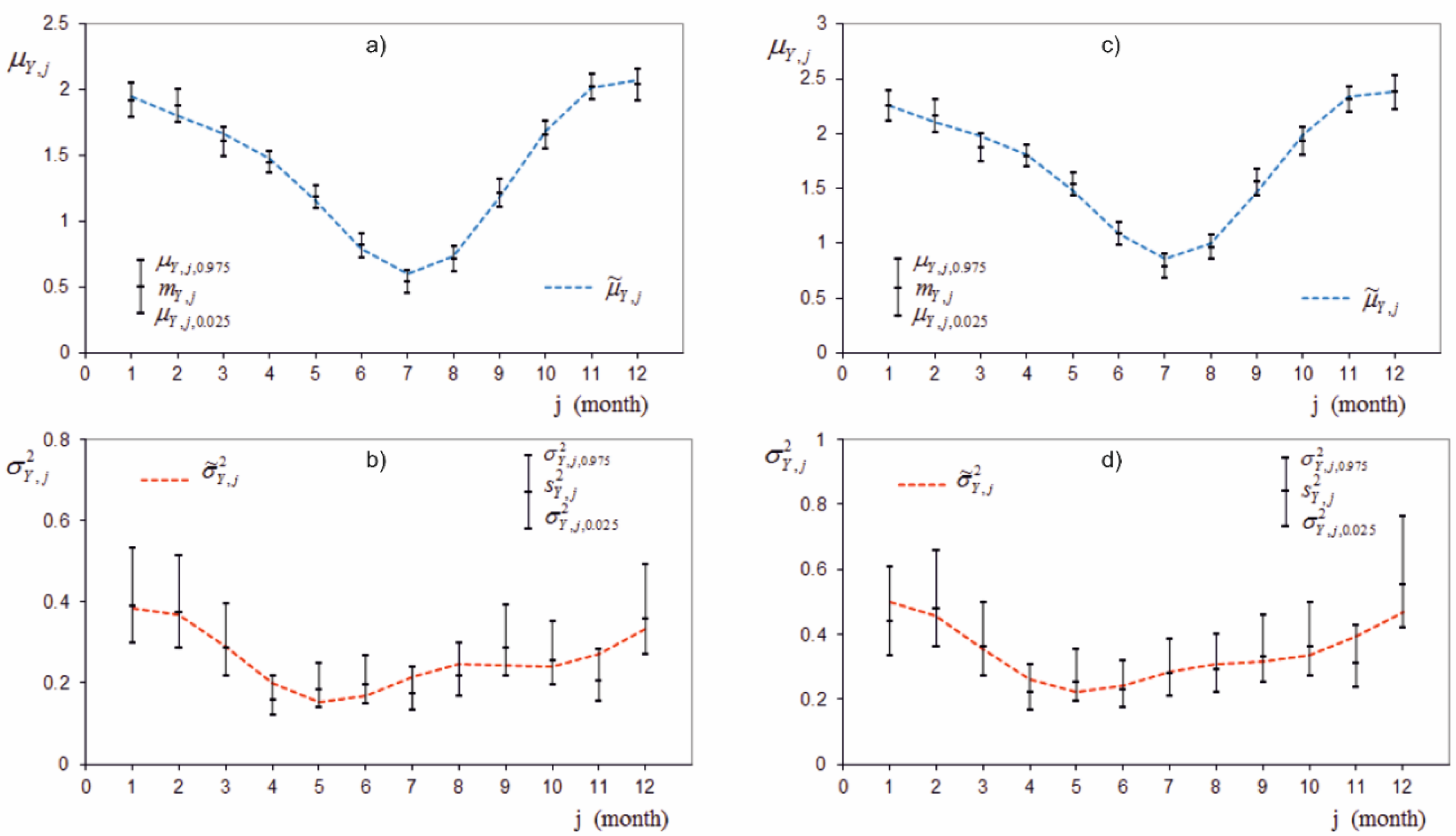
Different results have been obtained for the variance function (
Table 4). In fact, 1 harmonic has been evaluated for 3 out of 12 rain gauges, 2 harmonics for 7 rain gauges, and 3 harmonics for the other 2 rain gauges. Moreover, the comparisons among the observed values,
and
, the modeled values,
and
, and the dimension of the non-rejection intervals of the hypotheses
and
are shown in
Figure 2 for the Cosenza and Campotenese C.C. rain gauges.
Figure 2.
Comparison among the observed values, the modeled values, and the ranges (identified by the whiskers of the error bar) of the non-rejection regions of the hypotheses and , for the mean (blue) and the variance (red) functions, evaluated for the Cosenza (a,b) and the Campotenese C.C. (c,d) rain gauges.
By using the estimated values of the parameters, and by means of Equation (2), it was possible to build the observed sample
zk, with zero mean and unit variance, and the sample coefficients of skewness,
g1,Z, and kurtosis,
g2,Z. These values have been used to test the Gaussianity of the process
Zk, by verifying the non-rejection of the hypotheses
and
(
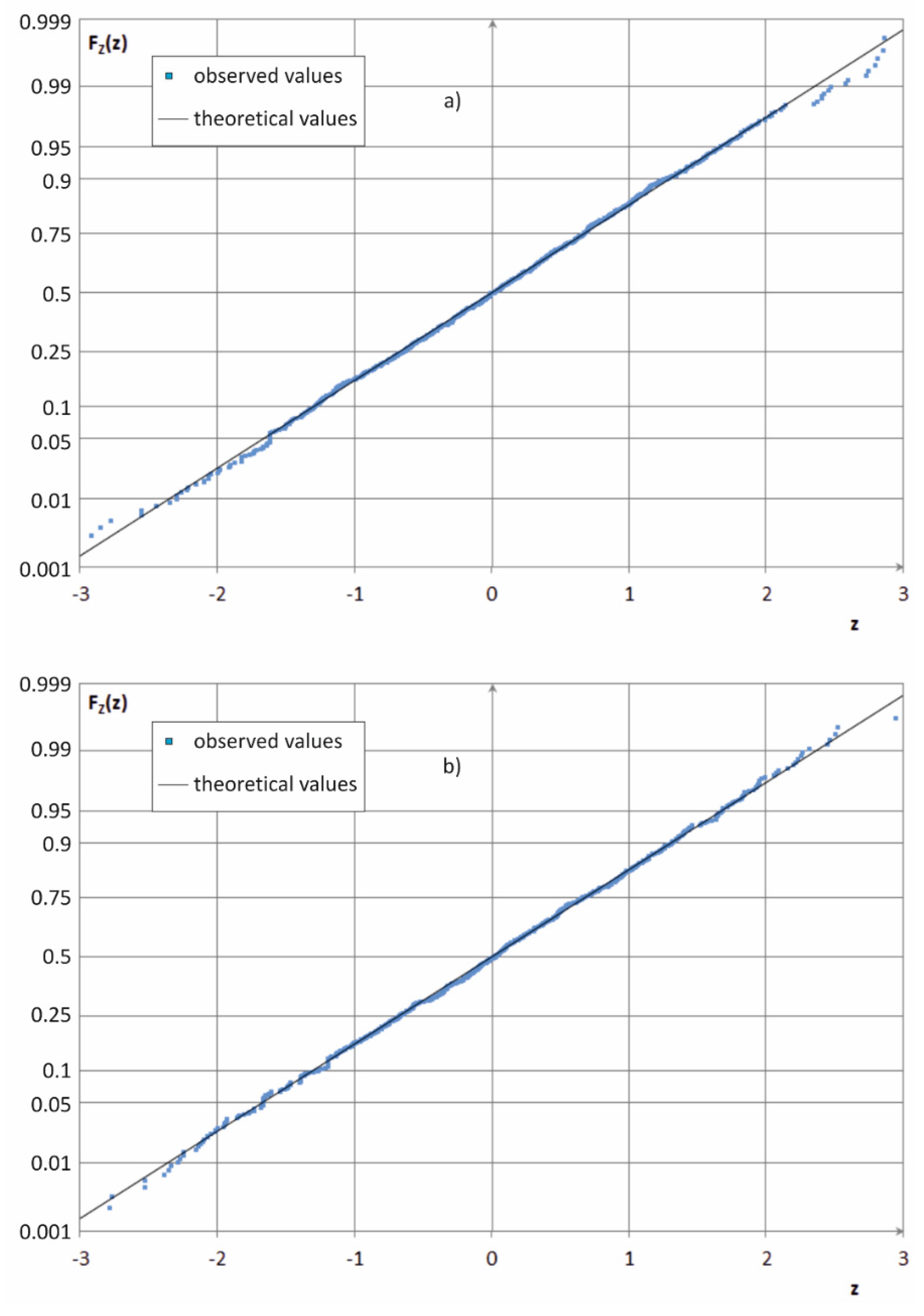
Table 5). Moreover, the comparisons between the cumulative frequency of the observed values and the cumulative distribution function (cdf) of the standardized Gaussian law have been reported in
Figure 3, for the Cecita ex Acquacalda and Scilla rain gauges. The non-rejection of the hypotheses
and
and the good fitting with the observed values (
Figure 3) confirm the goodness of the Gaussianization of the
Zk process.
Table 5.
Gaussianity test based on the coefficients of skewness and kurtosis.
Table 5.
Gaussianity test based on the coefficients of skewness and kurtosis.
| Rain Gauge | | | | | | |
|---|
| Campotenese | 1055 | −0.006 | ±0.148 | 2.731 | 2.813 | 3.315 |
| Capo Spartivento | 957 | −0.005 | ±0.155 | 2.718 | 2.857 | 3.333 |
| Cassano allo Jonio | 969 | −0.005 | ±0.154 | 2.720 | 2.746 | 3.331 |
| Cecita | 985 | 0.012 | ±0.153 | 2.722 | 3.114 | 3.328 |
| Cittanova | 1020 | −0.001 | ±0.151 | 2.726 | 3.164 | 3.321 |
| Cosenza | 1112 | −0.028 | ±0.144 | 2.738 | 2.814 | 3.304 |
| Filadelfia | 1067 | −0.001 | ±0.147 | 2.732 | 2.994 | 3.313 |
| Isola Capo Rizzuto | 962 | −0.013 | ±0.155 | 2.719 | 2.828 | 3.332 |
| Joppolo | 968 | 0.008 | ±0.154 | 2.720 | 3.184 | 3.331 |
| S.Pietro in Guarano | 1047 | 0.005 | ±0.149 | 2.730 | 3.046 | 3.316 |
| Scilla | 857 | 0.000 | ±0.162 | 2.706 | 2.951 | 3.352 |
| Tiriolo | 827 | 0.001 | ±0.165 | 2.702 | 3.021 | 3.357 |
For all the rain gauges, the sequences of observed values zk show low linear correlation coefficients, but they are not low enough to consider the process Zk uncorrelated. In fact, the application of the Anderson test, with a lag νmax = 24, to the zk series, evidenced that the hypothesis of uncorrelated process is non-rejectable only for the Cassano allo Jonio, Capo Spartivento and Joppolo rain gauges.
For the other 9 rainfall series, in order to describe the correlative structure, it was sufficient to adopt an autoregressive model of order
p = 1. In fact, after the estimation of the parameters
and
, the application of the Anderson test, always till a lag ν
max = 24, to the sequence of the sample bias
, showed the non-rejectability of the hypothesis of uncorrelated process.
Table 6 shows a synthesis of the application of the Anderson test to the selected 12 rain gauges, limited only to the lag ν = 1.
Table 6.
Anderson test applied to the autocorrelation coefficient of lag ν = 1.
Table 6.
Anderson test applied to the autocorrelation coefficient of lag ν = 1.
| Rain Gauge | | | | | | | | |
|---|
| Campotenese | −0.062 | 0.070 | 0.060 | rejected | −0.062 | −0.004 | 0.060 | not rejected |
| Capo Spartivento | −0.065 | 0.005 | 0.063 | not rejected | ----- | ----- | ----- | ----- |
| Cassano allo Jonio | −0.065 | 0.042 | 0.063 | not rejected | ----- | ----- | ----- | ----- |
| Cecita | −0.064 | 0.067 | 0.062 | rejected | −0.064 | 0.003 | 0.062 | not rejected |
| Cittanova | −0.063 | 0.113 | 0.061 | rejected | −0.063 | −0.004 | 0.061 | not rejected |
| Cosenza | −0.060 | 0.065 | 0.058 | rejected | −0.060 | 0.004 | 0.058 | not rejected |
| Filadelfia | −0.062 | 0.117 | 0.060 | rejected | −0.062 | −0.008 | 0.060 | not rejected |
| Isola Capo Rizzuto | −0.065 | 0.073 | 0.063 | rejected | −0.065 | 0.007 | 0.063 | not rejected |
| Joppolo | −0.064 | 0.061 | 0.062 | not rejected | ----- | ----- | ----- | ----- |
| S.Pietro in Guarano | −0.062 | 0.097 | 0.060 | rejected | −0.062 | −0.011 | 0.060 | not rejected |
| Scilla | −0.069 | 0.154 | 0.066 | rejected | −0.069 | −0.017 | 0.066 | not rejected |
| Tiriolo | −0.070 | 0.103 | 0.068 | rejected | −0.070 | −0.013 | 0.068 | not rejected |
Figure 3.
Comparison between the cumulative frequency of the observed values and the cdf of the standardized Gaussian law for the Cecita ex Acquacalda (a) and Scilla (b) rain gauges.
Figure 3.
Comparison between the cumulative frequency of the observed values and the cdf of the standardized Gaussian law for the Cecita ex Acquacalda (a) and Scilla (b) rain gauges.
4. Results and Discussion
After the parameter estimation by means of the selected rainfall database, 104 years long synthetic series have been generated for each rain gauge through a Monte Carlo procedure, reproducing the proposed model.
Then, the SPI was evaluated at two different time scales: 3-month SPI, which reflects short- and medium-term moisture conditions, and 12-month SPI, which is linked to long-term precipitation patterns and can impact on streamflows, reservoir levels, and even groundwater levels. The results obtained in terms of the occurrence probabilities of wet and dry conditions were compared with the class probability shown in
Table 1.
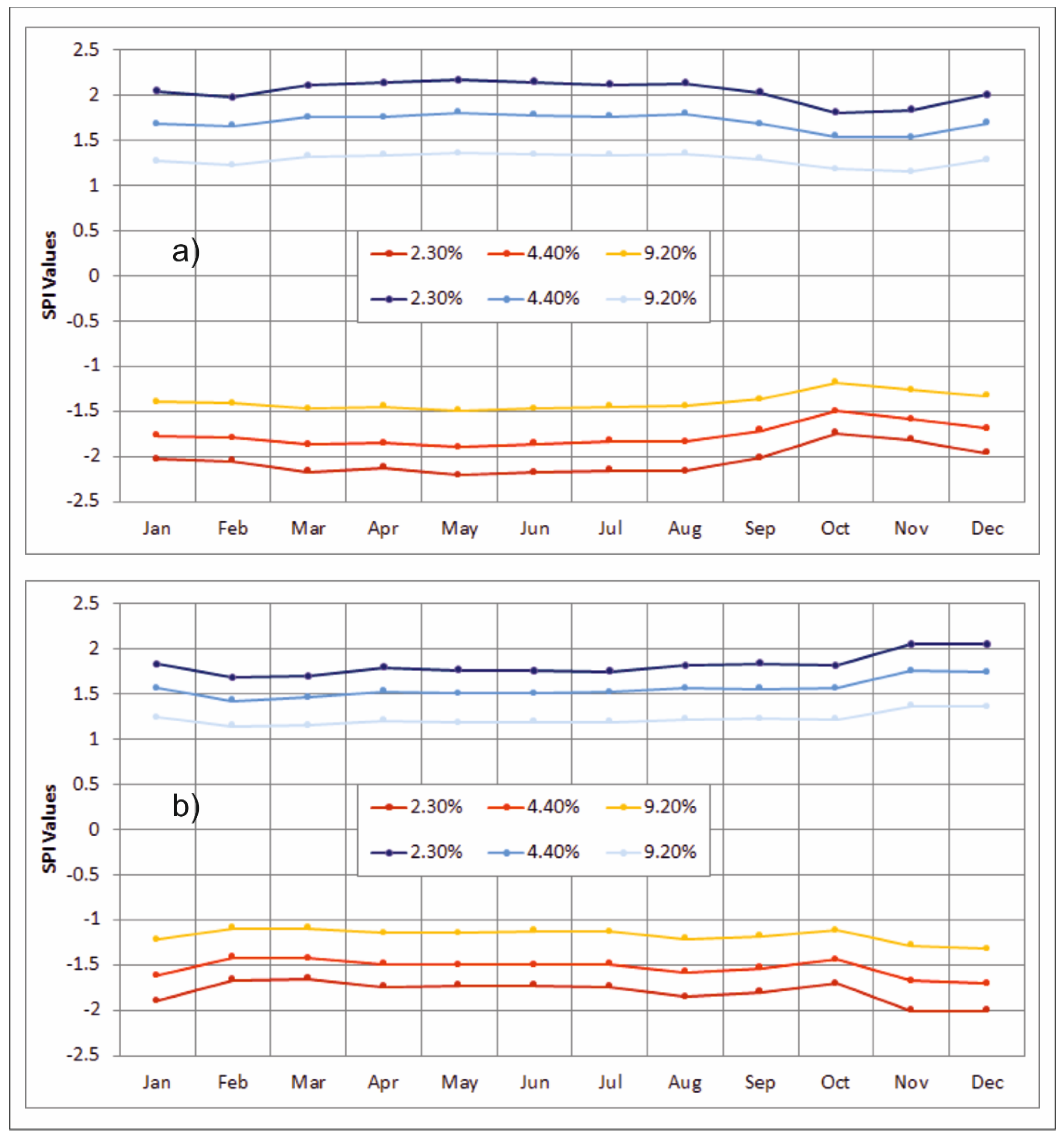
In
Figure 4, the results of the 12-month SPI for two rain gauges are shown (Isola di Capo Rizzuto and Capo Spartivento).
Figure 4.
Values of the 12-month SPI for fixed monthly occurrence probabilities of wet and dry conditions, evaluated for the simulated data of the Isola di Capo Rizzuto (
a) and the Capo Spartivento (
b) rain gauges. According to the theoretical values proposed in another publication [
86], each color identifies the prefixed value of the occurrence probability of wet (blue scale) and dry (red scale) conditions.
In this figure, by means of the simulated data, the SPI values corresponding to the probability of extreme (2.3%), severe (4.4%) and moderate (9.2%) conditions have been detected for each month. As a result, the probabilities proposed in another publication [
86] in the evaluation of the SPI were quite different from the ones obtained by the application of the SPI to the 10
4 simulated years. For example, for the Isola di Capo Rizzuto rain gauge (
Figure 4a), the occurrence probabilities of the extreme values confirmed the correspondent SPI values previously proposed [
86], while the severe and moderate probabilities values showed a different behavior. Similarly, for the Capo Spartivento rain gauge (
Figure 4b), the extreme and moderate probabilities differed from the correspondent SPI values proposed in
Table 1, while only the severe probabilities agree with them. This is very important, since for most practical applications the SPI is essential in terms of classification (
Table 1) and not as arithmetic values [
87].
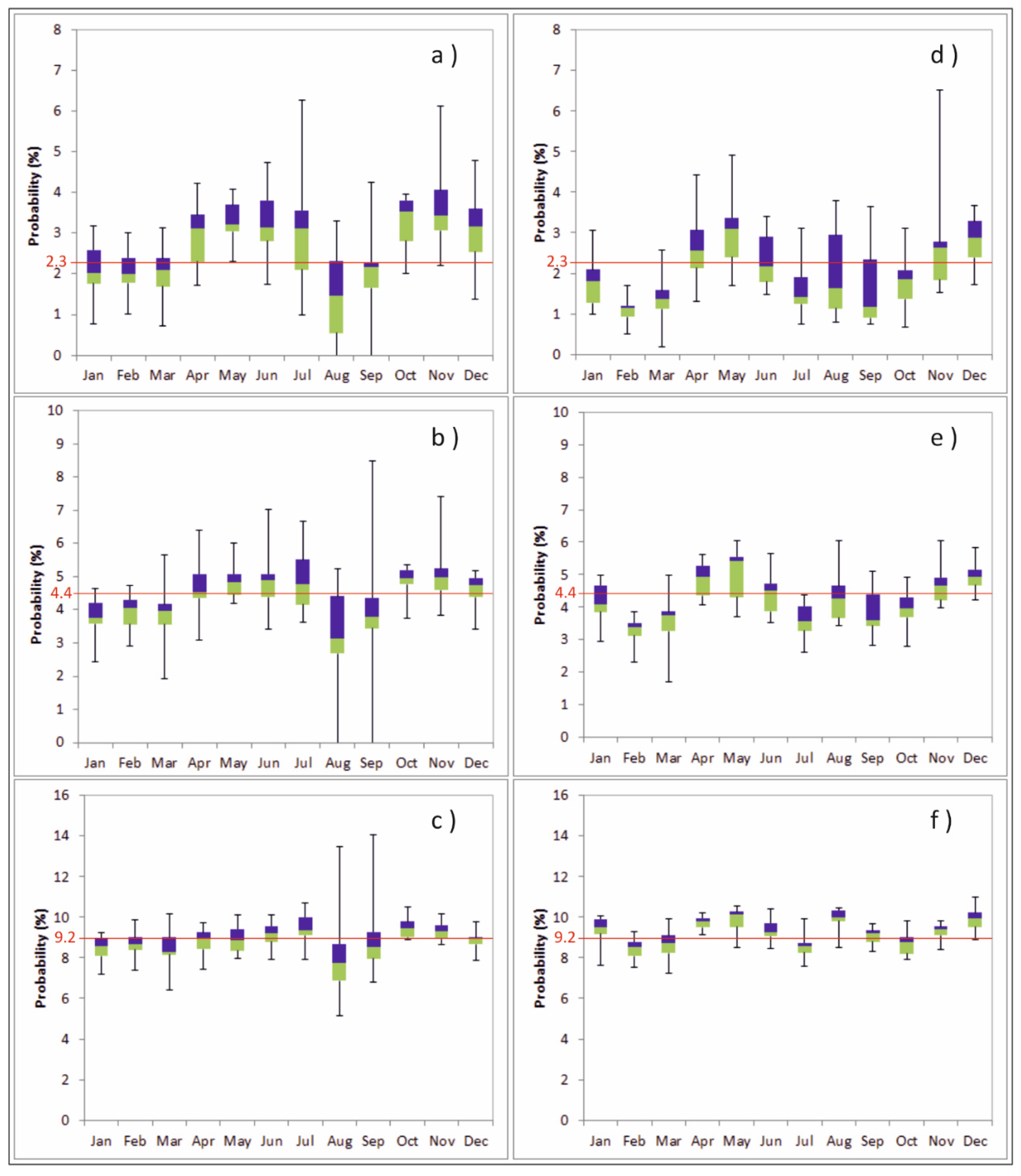
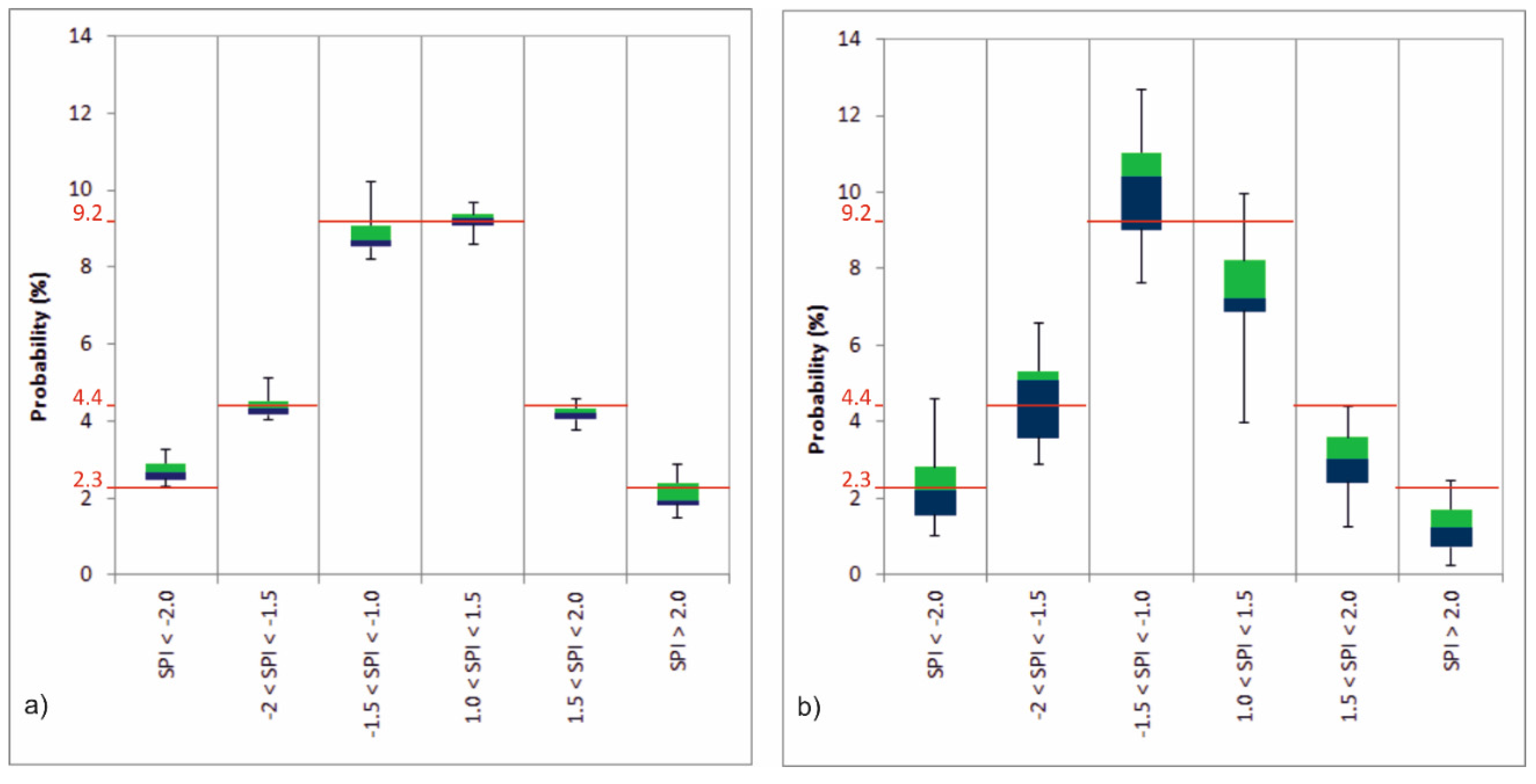
As regards to the 3-month-SPI,
Figure 5 presents some box plots that summarized the regional monthly occurrence probabilities of the different wet and dry classes. In particular, the box plots corresponding to extreme, severe and moderate dry and wet conditions have been shown together with the theoretical values proposed by [
86]. From these analyses it has emerged that in Calabria, as in other Italian regions [
43], the highest probability to detect extreme drought (
Figure 5a) or severe drought (
Figure 5b) conditions, were mainly observed in the wet seasons and, in particular, in the autumn period. In fact, the autumn and the spring months showed the highest values of the mean occurrence probabilities of drought, while the minimum values have been detected in August.
Figure 5.
Box-plots of the regional monthly occurrence probabilities of extreme drought (
a); severe drought (
b); moderate drought (
c); extremely wet (
d), severely wet (
e) and moderately wet (
f) conditions for the 3-month SPI. The red lines indicate the theoretical values proposed by [
86]. The bottom and top of the box are the first and third quartiles, the band inside the box is the median, the ends of the whiskers represent the minimum and maximum of all of the data.
Moreover, in the summer period, the occurrence probabilities of drought conditions showed a high regional variability, with large difference values between the several rain gauges. Conversely, the highest probability to detect extremely wet (
Figure 5d) or severely wet (
Figure 5e) conditions, were mainly observed in winter. No remarkable differences emerged for the moderate dry (
Figure 5c) and wet (
Figure 5f) conditions.
With regards to the comparison between the occurrence probabilities of wet and dry conditions evaluated from the simulated data and the class probability shown in
Table 1, the different dry and wet mean occurrence values generally fluctuate around the values proposed by [
86], but higher probability of extreme drought (
Figure 5a) can be observed.
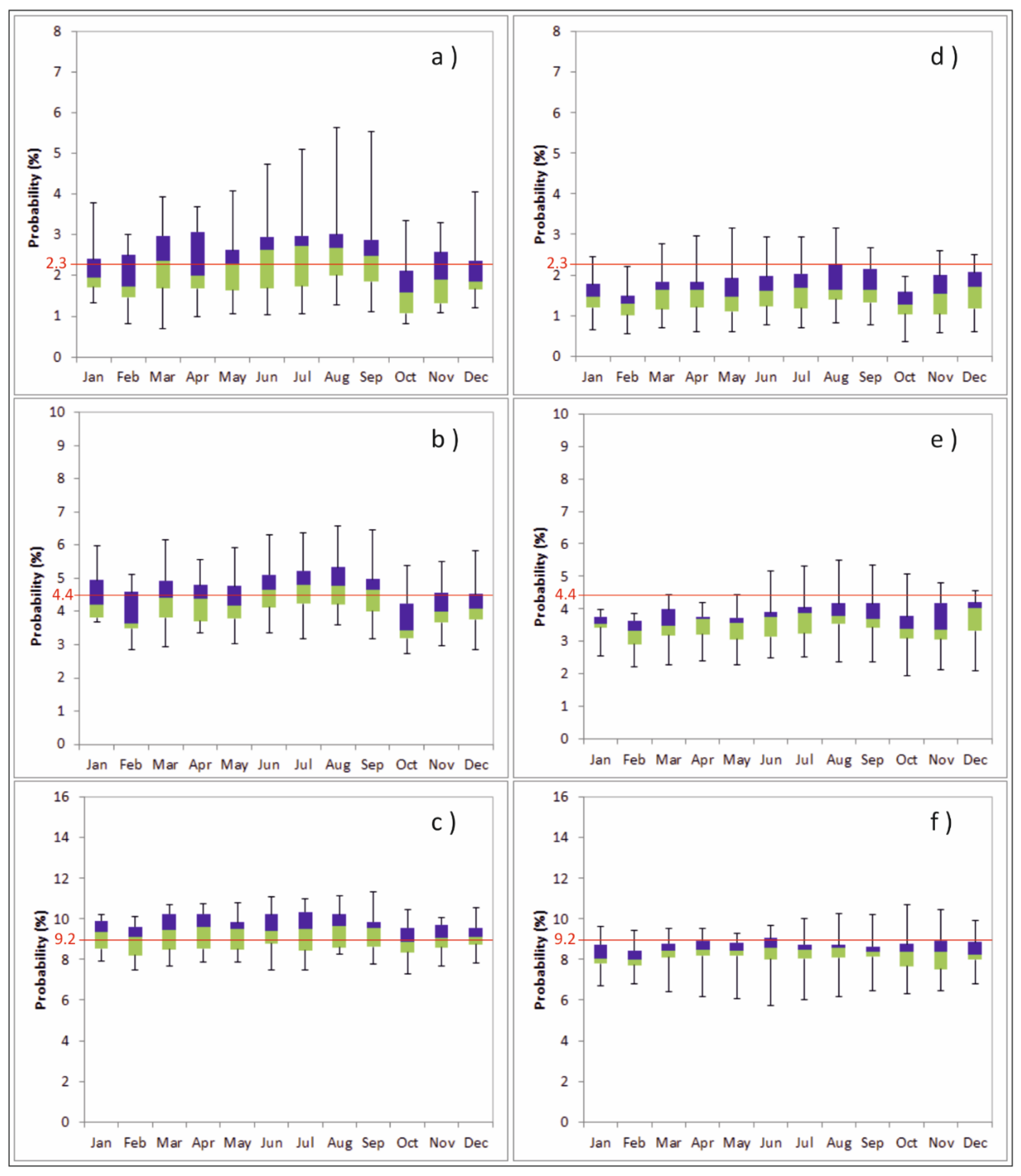
Similarly to
Figure 5, also for the 12-month SPI, the box plots with the regional monthly occurrence probabilities of the different wet and dry classes have been evaluated (
Figure 6). As opposed to
Figure 5, in these box plots there are few differences between the occurrence probabilities evaluated in the different months, in particular for the dry conditions. In fact, highest probabilities to detect extreme drought (
Figure 6a) or severe drought (
Figure 6b) conditions can be observed in the summer period. Moreover, only for the extreme drought (
Figure 6a) and in the summer period, the occurrence probabilities of drought conditions showed a high regional variability. The most important result of the 12-month SPI analysis emerged from the comparison between the occurrence probabilities of wet and dry conditions evaluated from the simulated data and the class probability shown in
Table 1. In fact, the extreme (
Figure 6a) and the severe drought (
Figure 6b) mean occurrences values generally fluctuate around the values proposed by [
86], and the moderate drought (
Figure 6c) presented slightly higher mean occurrences values than these. By contrast, the wet conditions (
Figure 6d–f) always showed lower mean occurrences values than those presented in
Table 1.
Figure 6.
Box-plots of the regional monthly occurrence probabilities of extreme drought (
a); severe drought (
b); moderate drought (
c), extremely wet (
d); severely wet (
e) and moderately wet (
f) conditions for the 12-month SPI. The red lines indicate the theoretical values proposed by [
86]. The bottom and top of the box are the first and third quartiles, the band inside the box is the median, the ends of the whiskers represent the minimum and maximum of all of the data.
These results indicate greater probability of dry conditions than wet conditions when long-term precipitation patterns are considered, with consequences on streamflows, reservoir levels, and groundwater levels.
Generally, from the box plots of
Figure 5 and
Figure 6, it can be observed that the 3-month SPI does not greatly vary in comparison to the 12-month SPI. The only exception are the box plots which refer to the extreme wet conditions (
Figure 5d and
Figure 6d) where, in 10 out of 12 months, the probability of the 3-month SPI evidenced a greater spread than the 12-month SPI. These results agree with the ones shown in
Figure 7 and with past studies in the region of Calabria [
41,
42], which evidenced that there is a great spatial heterogeneity of the SPI12 while the SPI3 shows a spatial homogeneity. Moreover, as a further result, the model spreads higher in summer than in the other seasons. This result can be due to the Mediterranean climate of the region, which shows high climatic variability with a typically dry summer subtropical climate. The rain gauges with the higher spread in summer are located in the Ionian side of the region, which is influenced by currents coming from Africa and is characterized by short and heavy precipitation in particular in the summer period.
Figure 7.
Box-plots of the regional occurrence probabilities of extreme, severe and moderate drought and wet conditions for the 3-month SPI (
left) and the 12-month SPI (
right). The lines indicate the theoretical values proposed by [
86]. The bottom and top of the box are the first and third quartiles, the band inside the box is the median, the ends of the whiskers represent the minimum and maximum of all of the data.
Figure 7 shows the box plots with the occurrence probabilities of the different wet and dry classes evaluated for the whole data series.
In particular, for the 3-month SPI (
Figure 7a), there are no marked differences between the evaluated mean occurrences probabilities and the ones previously proposed [
86], and the same happens between the occurrence probability of the corresponding dry/wet classes. Instead, for the 12-month SPI (
Figure 7b) strong differences between the evaluated mean occurrences probabilities and the ones shown in
Table 1 have been detected, with the drought and wet conditions which present respectively higher and lower values than the ones previously proposed [
86].
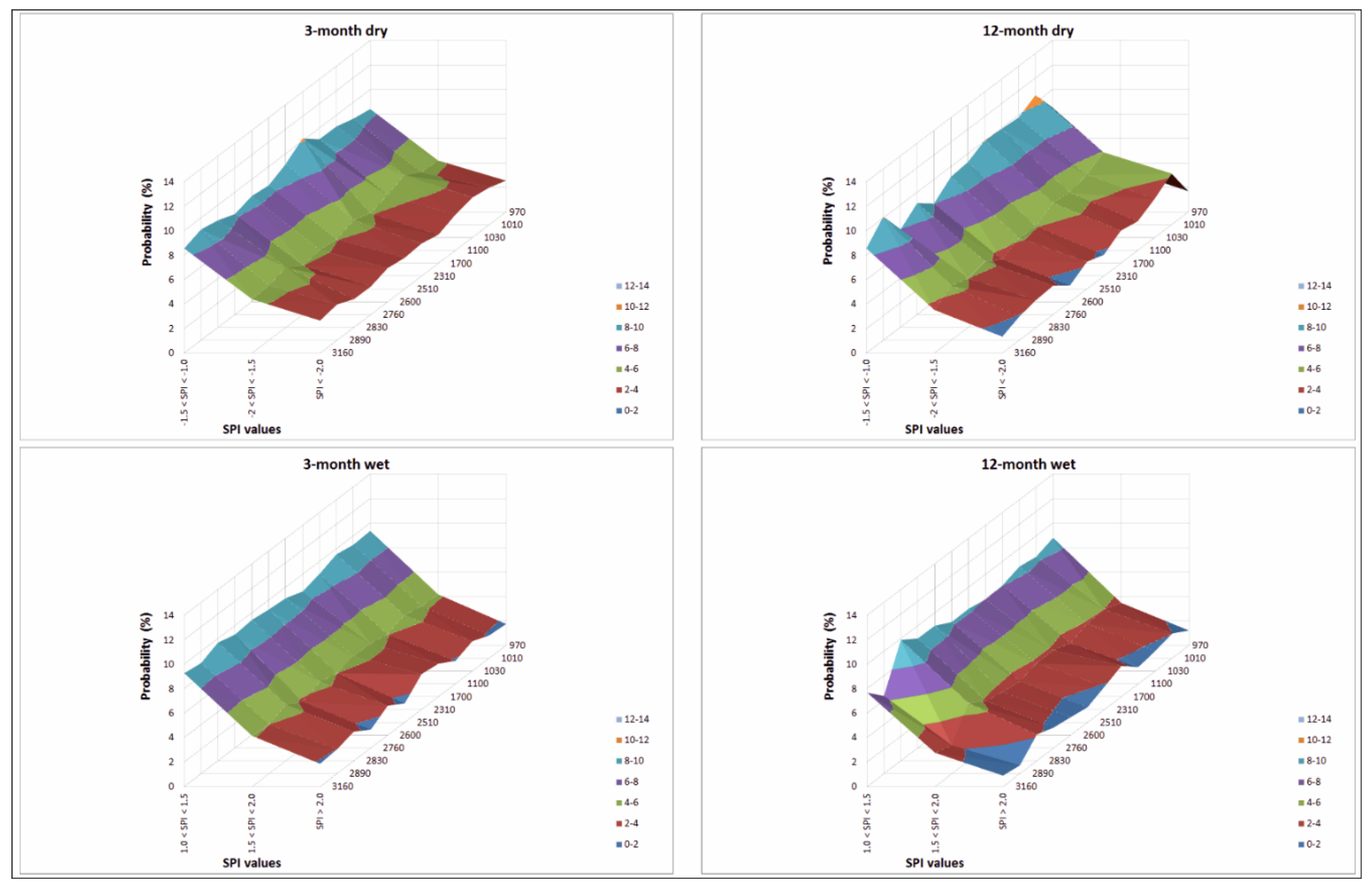
Detailed results for each rain gauge have been shown in
Table 7. The results confirm more chance for dry conditions than wet conditions when long-term precipitation patterns are considered. In fact, for almost all the rain gauges, the lowest probability values have been detected for the wet conditions, while the highest probability values have been detected for the dry conditions. For example, for the Cosenza rain gauge (code 1010), the probabilities that the 12-month SPI belong to the extreme classes (SPI < −2 and SPI > 2) are 4.2% and 2.0%, respectively. The same happens for the severe SPI classes (−2 < SPI < −1.5 and 1.5 < SPI < 2) where dry conditions show higher probabilities (5.9%) than wet conditions (4.0%). A similar behavior is shown by the 3-month SPI, even though with lower marked differences between dry and wet conditions (
Table 7). These results, which evidence the highest probability values evaluated for the dry conditions, are visually described in
Figure 8. The different colors of the figure represent several probability classes. In fact, the colors associated to the ranges with higher probabilities can be observed only for dry conditions. On the contrary, the lower probability classes can be identified mainly for the wet conditions.
Table 7.
Probability of the simulated data to fall within each SPI class evaluated for each rain gauge.
Table 7.
Probability of the simulated data to fall within each SPI class evaluated for each rain gauge.
| Months | SPI Class | 970 | 1010 | 1030 | 1100 | 1700 | 2310 | 2510 | 2600 | 2760 | 2830 | 2890 | 3160 |
|---|
| 3 | SPI < −2 | 2.6 | 3.0 | 3.3 | 2.9 | 2.3 | 2.7 | 2.5 | 2.7 | 2.3 | 2.3 | 2.9 | 2.6 |
| −2<SPI< −1.5 | 4.2 | 4.3 | 5.1 | 4.5 | 4.1 | 4.6 | 4.0 | 4.2 | 4.0 | 4.9 | 4.5 | 4.4 |
| −1.5 < SPI < −1 | 8.4 | 8.7 | 9.1 | 9.1 | 10.2 | 9.2 | 8.5 | 8.6 | 8.2 | 8.8 | 9.1 | 8.5 |
| 1 < SPI < 1.5 | 9.4 | 9.3 | 9.5 | 9.0 | 8.6 | 9.1 | 9.2 | 9.4 | 9.3 | 9.7 | 9.0 | 9.3 |
| 1.5 < SPI < 2 | 4.2 | 4.3 | 4.6 | 4.0 | 4.3 | 4.3 | 4.0 | 4.3 | 3.8 | 4.6 | 4.0 | 4.1 |
| SPI > 2 | 1.7 | 1.9 | 2.4 | 1.9 | 2.7 | 2.9 | 1.5 | 2.4 | 1.5 | 2.4 | 2.0 | 1.8 |
| 12 | SPI < −2 | 1.7 | 4.2 | 3.1 | 2.4 | 2.7 | 1.7 | 2.2 | 1.3 | 2.4 | 2.2 | 1.9 | 1.3 |
| −2 < SPI < −1.5 | 3.6 | 5.9 | 5.1 | 4.7 | 4.9 | 4.1 | 4.2 | 3.5 | 4.3 | 4.0 | 4.4 | 3.5 |
| −1.5 < SPI < −1 | 8.5 | 10.6 | 9.8 | 9.9 | 10.1 | 9.3 | 9.2 | 8.0 | 9.1 | 8.0 | 10.1 | 8.5 |
| 1 < SPI < 1.5 | 8.8 | 8.3 | 8.5 | 8.0 | 8.0 | 8.2 | 8.2 | 8.9 | 9.0 | 9.9 | 6.4 | 7.7 |
| 1.5 < SPI < 2 | 3.5 | 4.0 | 3.9 | 3.3 | 3.8 | 3.8 | 3.3 | 3.5 | 3.8 | 4.7 | 2.3 | 2.7 |
| SPI > 2 | 1.2 | 2.0 | 1.6 | 1.4 | 2.5 | 1.9 | 1.2 | 1.5 | 1.7 | 2.1 | 0.7 | 0.9 |
Figure 8.
Occurrence probabilities of extreme, severe and moderate drought and wet conditions for the 3-month SPI and the 12-month SPI for each rain gauge.
Figure 8.
Occurrence probabilities of extreme, severe and moderate drought and wet conditions for the 3-month SPI and the 12-month SPI for each rain gauge.
Some results obtained from the application of the SPI are confirmed by the DSI, evaluated for each rain gauge on two time scales (3 and 6 months) using the synthetic monthly precipitation series.
Table 8 compares the two indices (DSI3 and DSI6) at each location, in terms of percentages of months for which the drought severity index was negative, positive or equal to zero (no rainfall deficit). As was the case in a previous publication [
25], for all the rain gauges a six-monthly rule (DSI6) hinders the development of a drought sequence. In fact, the deficit emerges considering rainfall behavior over three, rather than six months with a maximum percentage decrease of 9% (ID 1700) passing from DSI3 to DSI6. The different results obtained with DSI6 also appear when DSI values equal to zero are considered. For DSI3 the percentages of months with positive values are always greater than those equal to zero. On the contrary, for DSI6 there are rain gauges for which months with DSI equal to zero are greater than those with positive values. Some of the DSI features confirm the results of SPI. For example, the probabilities of extreme drought for SPI on large scale (in this study, 12 month-SPI) are often lower than those relative to 3-month SPI. Moreover, some of the rain gauges with the highest probabilities of extreme drought are the same, showing high percentages with positive values of DSI3 (
i.e., ID 1030, 2310, 2600, 2890, 3160).
Table 8.
Percentages of the simulated monthly data to fall within each DSI class evaluated for each rain gauge.
Table 8.
Percentages of the simulated monthly data to fall within each DSI class evaluated for each rain gauge.
| DSI | DSI Class | 970 | 1010 | 1030 | 1100 | 1700 | 2310 | 2510 | 2600 | 2760 | 2830 | 2890 | 3160 |
|---|
| DSI3 | Negative | 0.5 | 0.4 | 0.4 | 0.5 | 0.5 | 0.5 | 0.3 | 0.4 | 0.4 | 0.4 | 0.3 | 0.3 |
| Positive | 56.1 | 53.5 | 57.0 | 50.5 | 55.9 | 59.5 | 58.9 | 63.1 | 56.0 | 55.6 | 62.5 | 65.2 |
| Zero | 43.4 | 46.0 | 42.6 | 49.0 | 43.6 | 40.0 | 40.7 | 36.6 | 43.6 | 44.0 | 37.1 | 34.5 |
| DSI6 | Negative | 0.9 | 1.0 | 0.9 | 0.9 | 0.9 | 0.8 | 0.8 | 0.8 | 0.9 | 0.9 | 0.8 | 0.7 |
| Positive | 52.0 | 48.3 | 52.7 | 43.5 | 46.9 | 54.5 | 55.0 | 59.3 | 50.5 | 49.3 | 59.7 | 64.0 |
| Zero | 47.1 | 50.7 | 46.4 | 55.6 | 52.3 | 44.7 | 44.2 | 39.9 | 48.6 | 49.8 | 39.5 | 35.3 |
The results of this paper confirm that, due to the long-term trend of global warming, there is a higher chance of dry conditions than of wet conditions [
106,
107]. This is a critical issue for an agricultural region, such as Calabria, that suffers climate change [
108,
109,
110], which is a major driver of agricultural and meteorological drought. In fact, precipitation and temperature anomalies caused by climate change will induce agro-meteorological drought [
111]. In addition, water is usually significantly contaminated by organic matter derived from agricultural production and sewage, which may further aggravate the agricultural drought risk [
112].
5. Conclusions
Unlike most natural hazards such as earthquakes and cyclones, both of which can strike quickly, drought does not usually have a sudden beginning or end. It is an insidious hazard caused by a period of abnormally dry weather, persisting long enough to produce a serious hydrologic imbalance. While a drought is unlikely to cause human deaths in most developed countries, a drought in a developing country without adequate access to aid can be devastating. In fact, drought can often be a natural hazard with the biggest economic impact, resulting in very costly and dramatic impacts on the environment such as stock losses, vulnerability to fires (especially in forested areas), crop damage, soil erosion, power blackouts if your community is reliant on electricity from hydro dams, and water supply shortages. The severity of a drought depends upon the degree of moisture deficiency, duration, and size of the affected area.
Monitoring dry and wet periods using meteorological indices, such as rainfall, is an essential component for drought preparedness. The variability of the rainfall is intrinsically present in its process, and it places uncertainties on projections. The use of the stochastic approach and the simulation procedure can effectively generate the variability of the rainfall process, and addresses the problem of quantity and reliability of the data used to fit the rainfall distribution. In the present paper, a model of monthly precipitation has been proposed. It adopts variable transformations, finalized to the deseasonalization and to Gaussianization of the monthly rainfall process, and includes a procedure for testing the autocorrelation. The model provided a good representation of the monthly rainfall for the selected 12 rain gauges of Calabria (Southern Italy). For this reason, 104-year-long synthetic series have been generated for each rain gauge through a Monte Carlo procedure, and dry and wet periods in the region of Calabria were analyzed using the SPI applied to the simulated series. The index was calculated at two different time scales: 3-month SPI, which reflects short and medium-term moisture conditions, and 12-month SPI, which is linked to long-term precipitation patterns and can have an impact on streamflows, reservoir levels, and even groundwater levels. The occurrence probabilities of extreme, severe and moderate wet and dry conditions have been evaluated for each month, and compared with the corresponding probability classes commonly adopted in the literature. The comparison evidenced some differences, in particular for the 12-month SPI, for which higher probability values for dry conditions and lower probability values for wet conditions have been detected. Analogous results, as further confirmation of the good representation provided by the proposed model, have been obtained by means of the application of the DSI, based on the accumulated monthly rainfall deficits evaluated through the precipitation anomalies.
The advantage of the proposed model is that the stochastic approach overcomes the problems of quantity and reliability of the data, and can well reproduce the statistical characteristics of observed data, thus allowing a better prediction of the occurrence probabilities of extreme dry/wet conditions. Moreover, the stochastic model has the advantage of being applicable everywhere and for any gauge, because it does not depend on station altitude and climatic zone. For its characteristics, the model can also be applied to precipitation monthly grids, but this application depends on the grid size. In fact, the whole procedure is highly time-consuming, and its application is not recommended for too detailed grid sizes. Anyway, the proposed model can be considered an attractive tool for management decision-making, allowing the identification of a drought risk. Finally, properly adapted, the model can also be applied together with the climate projection obtained from global circulation models as a reliable tool for drought estimation in a changing climate.


