Multilayer Numerical Modeling of Flows through Vegetation Using a Mixing-Length Turbulence Model

Abstract

This work focuses on the effects of vegetation on a fluid flow pattern. In this numerical research, we verify the applicability of a simpler turbulence model than the commonly used k-ε model to predict the mean flow through vegetation. The novel characteristic of this turbulence model is that the horizontal mixing-length is explicitly calculated and coupled with a multi-layer approach for the vertical mixing-length, within a general three-dimensional eddy-viscosity formulation. This mixing-length turbulence model has been validated in previous works for different kinds of non-vegetated flows. The hydrodynamic numerical model used for simulations is based on the Reynolds-averaged Navier–Stokes equations for shallow water flows, where a vegetation shear stress term is considered to reproduce the effects of drag forces on flow. A second-order approximation is used for spatial discretization and a semi-implicit Lagrangian–Eulerian scheme is used for time discretization. In order to validate the numerical results, we compare them against experimental data reported in the literature. The comparisons are carried out for two cases of study: submerged vegetation and submerged and emergent vegetation, both within an open channel flow.

1. Introduction

Natural river floodplains and adjacent wetlands have vital ecological functions in riverine landscapes [1,2]. Their vegetation typically comprises a diverse and heterogeneous combination of herbs, shrubs and trees, which influence sediment, nutrient and pollutant transport [3]. Vegetation is thus a key factor in the interrelated systems of flow, sediment transport and geomorphology in rivers [4]. While the hydraulic resistance of solid boundaries with small-scale irregularities is quite well understood, situations in which resistance elements are of similar size to the flow depths still pose large problems [5]. The effects of vegetation on flow are significant and cause difficulties in hydraulic design. Near the roughness tops especially, the general form of the most representative velocity profile is still a matter of debate [6–9]. Generally, non-submerged and submerged conditions are distinguished. When the vegetation is non-submerged, the flow is, in some measure, obstructed by vegetation over the entire water column. When the vegetation is submerged, a free-stream layer is observed near the free surface.

There are two ways to determine the hydrodynamics and the shear stress caused by the presence of vegetation in flow: physical experiments and analytical and numerical models. Freeman et al. [10] experimentally investigated the effect of vegetation on flow and developed regression equations for both partially-submerged and fully-submerged vegetation in terms of the characteristics of the plants and the flow regime. Järvelä [11] experimentally analyzed the flow resistance of natural floodplain plants and showed that friction factors and drag coefficients present variations as a function of the Reynolds number, the flow depth, the flow velocity and the characteristics of plants. The resolution of velocity profiles obtained from experiments strongly depends on the measurement equipment used. The electro-acoustic blanking of acoustic Doppler profilers (ADPs) causes significant loss of data, especially near the free surface and the bottom boundary layer. Other methods have been used in vegetated flow experiments to measure in regions where ADPs cannot, e.g., laser Doppler velocimetry (LDV) [3] or particle image velocimetry (PIV) [12].

Velocity distribution laws, such as the logarithmic distribution, have been shown to be useful for estimating velocity profiles above vegetation layers [13,14]. However, for deep submergence or protruding flexible vegetation, it is doubtful if the logarithmic velocity distribution exists in either a cycle-time averaged or an instantaneous sense, and the resistance to the flow is probably caused more by the form of the drag of the vegetation than by the bed shear [15].

Other authors perform hydrologic balances in order to determine flow characteristics; these include the WETFLOWmodel developed by Feng and Molz [16], the natural system model (NSM) developed by Fennema [17] and the South Florida Water Management model (SFWMM) developed by Lal [18]. These models are based on 2D nonlinear diffusion, which implies that the advection processes and turbulence are completely ignored. Other models numerically solve the hydrodynamic equations, including vegetation shear stress, such as the one-dimensional model of Rowinski and Kubrak [19], the two-dimensional model (depth-integrated) of Arega and Sanders [20] and the three-dimensional models of Fischer-Antze et al. [21], Choi and Kang [22] and others [23–25]. One of the difficulties in numerical modeling is to define a proper turbulence model. The k-ε model and similar models have been most widely employed to characterize flow through vegetation [26–28]. However, these models involve a level of uncertainty, since the empirical coefficients have not yet been satisfactorily obtained.

Other authors have applied algebraic and Reynolds stress models to study flow through vegetation. Naot et al. [29] carried out numerical simulations with an algebraic stress model to observe the impact of vegetation on the floodplain in the compound open-channel. Choi and Kang [22] used a Reynolds stress model for submerged vegetation in an open-channel flow, and their findings showed a better prediction of the mean velocity and turbulence intensity than the algebraic stress model or the k-ε model. Such models, however, require a very high computational cost, because of the number of equations that must be solved.

In studies by Alamatian and Jaefarzadeh [30], several numerical experiments were conducted using the finite triangular volume method with three turbulence models: mixing-length, k − ∊ and an algebraic stress model, which produced the best accuracy compared to experimental values. Similar studies by Akilli [31] and Fu [32,33] found that the k − ∊ model overestimates the speeds. Similarly, Sadeque et al. [34,35] reported similar results to those of Fu.

In the experiments of Rodi and Scheuerer [36], the k − ∊ model and a model consisting of a single equation were used to predict the adverse pressure gradients on border layers. The single equation model produced good results, but the k − ∊ model produced systematic discrepancies and excessive friction due to coefficients, especially in relatively simple fluxes. Lam and Bremhorst [37] showed that some simplifications of the k − ∊ model provide better results for semi-laminar and laminar fluxes in pipes compared to previous forms proposed by the k − ∊ model.

To avoid the difficulties posed by high-accuracy turbulence models, Gao [25] used and validated a simple two-layer mixing-length model, obtaining good agreement with measurements.

Despite the great number of versions of turbulence models based mainly on mixing-length, k − ∊ and algebraic methods, none can be used universally for all kinds of problems, as the scale of the study domain and the available computer equipment must be considered.

In the present work, we verify the applicability of a simpler turbulence model than the commonly used k − ∊ model to predict the mean 3D flow through vegetation. A more sophisticated mixing-length model for turbulence than the model used by Gao [25] is used. The two-layer mixing-length model proposed by Stansby [38] is considered. The novel characteristic of this turbulence model is that the horizontal mixing length is explicitly defined as a multiple of the vertical mixing length within a general three-dimensional eddy-viscosity formulation. Flow effects caused by the height of vegetation are characterized by a multilayer approach. Since natural flows through vegetation are, in general, shallow-water bodies, the current numerical model considers the hydrostatic approximation and solves the shallow-water equations. The formulation presented by Freeman [10] was adapted to include the vegetation shear stress in the velocity equations. The vegetation shear stress is a function of the characteristic dimensions of the plants, their flexibility and the vegetation density. Numerical simulations are carried out in order to validate the present turbulence model and to show its scope. Two cases of study are defined for this purpose: a channel flow with submerged vegetation; and a channel flow with both submerged and emergent vegetation. The calculation of correlation coefficients shows the accuracy of predictions against measurements.

2. Governing Equations

The system of equations used to calculate the velocity fields are the Reynolds-averaged Navier–Stokes equations for shallow-water flows. A correction term is considered in the velocity equations in order to characterize the shear stress due to the presence of vegetation. After turbulent averaging, the governing equations for the velocity components have the following form:

$$\begin{array}{l}\frac{\partial U}{\partial t}+U\frac{\partial U}{\partial x}+V\frac{\partial U}{\partial y}+W\frac{\partial u}{\partial z}=-\frac{\rho g}{{\rho }_0}\frac{\partial \eta }{\partial x}+\frac{\partial }{\partial x}\left(2{\nu }_E\frac{\partial U}{\partial x}\right)\\ \hspace{0.17em}\hspace{0.17em}\hspace{0.17em}\hspace{0.17em}\hspace{0.17em}\hspace{0.17em}\hspace{0.17em}\hspace{0.17em}\hspace{0.17em}\hspace{0.17em}\hspace{0.17em}\hspace{0.17em}\hspace{0.17em}\hspace{0.17em}\hspace{0.17em}\hspace{0.17em}\hspace{0.17em}\hspace{0.17em}\hspace{0.17em}\hspace{0.17em}\hspace{0.17em}\hspace{0.17em}\hspace{0.17em}\hspace{0.17em}\hspace{0.17em}\hspace{0.17em}\hspace{0.17em}\hspace{0.17em}+\frac{\partial }{\partial y}\left[{\nu }_E\left(\frac{\partial U}{\partial y}+\frac{\partial V}{\partial x}\right)\right]+\frac{\partial }{\partial z}\left({\nu }_E\frac{\partial U}{\partial z}\right)-\frac{1}{{\rho }_0}\frac{{\tau }_x^v}{\mathrm{\Delta }z},\end{array}$$

(1)

$$\begin{array}{l}\frac{\partial V}{\partial t}+U\frac{\partial V}{\partial x}+V\frac{\partial V}{\partial y}+W\frac{\partial V}{\partial z}=-\frac{\rho g}{{\rho }_0}\frac{\partial \eta }{\partial y}+\frac{\partial }{\partial y}\left(2{\nu }_E\frac{\partial V}{\partial y}\right)\\ \hspace{0.17em}\hspace{0.17em}\hspace{0.17em}\hspace{0.17em}\hspace{0.17em}\hspace{0.17em}\hspace{0.17em}\hspace{0.17em}\hspace{0.17em}\hspace{0.17em}\hspace{0.17em}\hspace{0.17em}\hspace{0.17em}\hspace{0.17em}\hspace{0.17em}\hspace{0.17em}\hspace{0.17em}\hspace{0.17em}\hspace{0.17em}\hspace{0.17em}\hspace{0.17em}\hspace{0.17em}\hspace{0.17em}\hspace{0.17em}\hspace{0.17em}\hspace{0.17em}\hspace{0.17em}\hspace{0.17em}+\frac{\partial }{\partial x}\left[{\nu }_E\left(\frac{\partial U}{\partial y}+\frac{\partial V}{\partial x}\right)\right]+\frac{\partial }{\partial z}\left({\nu }_E\frac{\partial V}{\partial z}\right)-\frac{1}{{\rho }_0}\frac{{\tau }_y^v}{\mathrm{\Delta }z},\end{array}$$

(2)

$$\frac{\partial W}{\partial z}=-\left(\frac{\partial U}{\partial x}+\frac{\partial V}{\partial y}\right),$$

(3)

where U, V and W are the mean velocity components in the x, y and z directions, respectively (m/s); g is the acceleration due to gravity (m/s²); ρ is the water density (kg/m³); ρ₀ is the water reference density (kg/m³); η is the free surface elevation (m); ν_E is the kinematic eddy viscosity (m²/s), which consists of turbulent and molecular components, such that ν_E = ν_t + ν; Δz is the height of the vegetation layer (m); and ${\tau }_x^v$ and ${\tau }_y^v$ are the vegetation shear stresses in the x and y directions, respectively (N/m²).

By integrating the continuity equation (Equation (3)) over the water depth and by using a kinematic condition at the free surface, the equation used to calculate the free surface elevation is:

$$\frac{\partial \eta }{\partial t}=-\frac{\partial }{\partial x}\left({\int }_{-h}^{\eta }U\mathit{dz}\right)-\frac{\partial }{\partial y}\left({\int }_{-h}^{\eta }V\mathit{dz}\right),$$

(4)

where h(x, y) is the water depth (m).

In Equations (1) and (2), the latter terms characterize the shear stress due to vegetation, which causes a decrease in the velocity field. These terms are neglected in regions without vegetation.

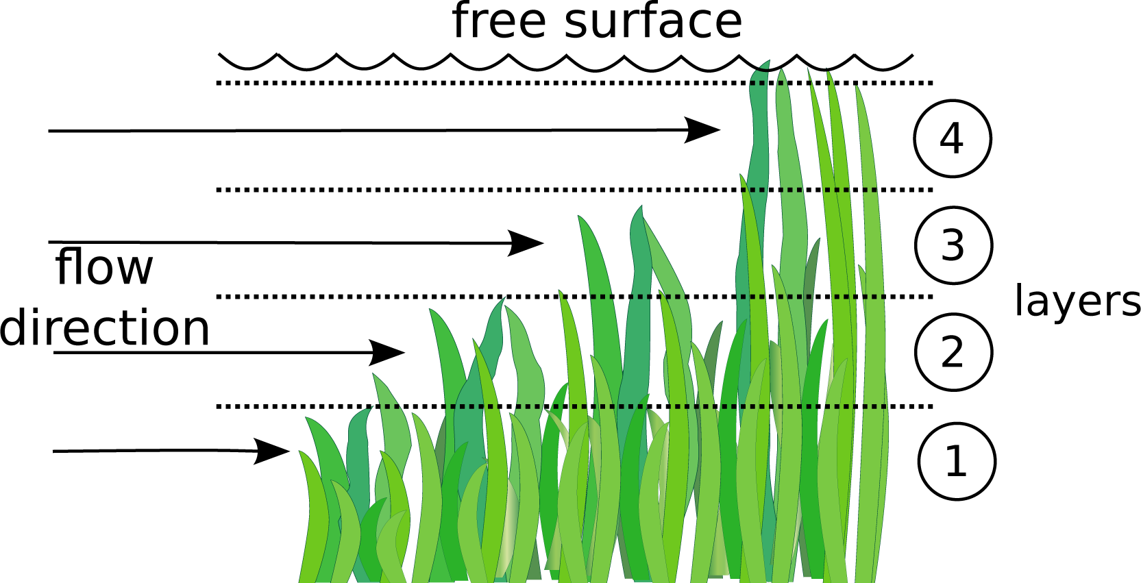
2.1. Turbulence Modeling

The simple two-layer mixing-length model for turbulence presented by Stansby [38] has been implemented in the current numerical model. The defining characteristic of this model is that the horizontal mixing length is explicitly made a multiple of the vertical mixing length within a general three-dimensional eddy-viscosity formulation. This means that the horizontal mixing length and associated strain rates determine the magnitude of the eddy-viscosity, which determines the degree of vertical mixing. The turbulent viscosity coefficient ν_t is then computed through the following mixing-length model:

$$\begin{array}{lll}{\nu }_t\hfill & =\hfill & \{l_h^4\left[2{\left(\frac{\partial U}{\partial x}\right)}^2+2{\left(\frac{\partial V}{\partial y}\right)}^2+{\left(\frac{\partial V}{\partial x}+\frac{\partial U}{\partial y}\right)}^2\right]\hfill \\ \hfill & \hfill & {+l_v^4\left[{\left(\frac{\partial U}{\partial z}\right)}^2+{\left(\frac{\partial V}{\partial z}\right)}^2\right]\}}^{1/2},\hfill \end{array}$$

(5)

where the vertical length scale l_v = κ(z−z_b) for (z−z_b)/δ < λ/κ, and l_v = λδ for λ/κ < (z−z_b)/δ < 1; κ is the von Kármán constant, typically 0.41; (z−z_b) is the distance from the wall; δ is the boundary-layer thickness; and λ is a constant, typically 0.09 [38]. In the case of shallow-water flows, due to the steady current, the boundary-layer thickness may be assumed to be equal to the water depth h. The horizontal length scale is usually different from the vertical length scale, and the simplest assumption is direct proportionality defined by l_h = βl_v. The constant β has to be determined experimentally. For parallel flow cases (or near-parallel), eddy viscosity reverts to its standard boundary-layer form. With l_h = l_v, it reverts to its correct mathematical three-dimensional form (with negligible vertical velocity).

2.2. Vegetation and Bottom Shear Stresses

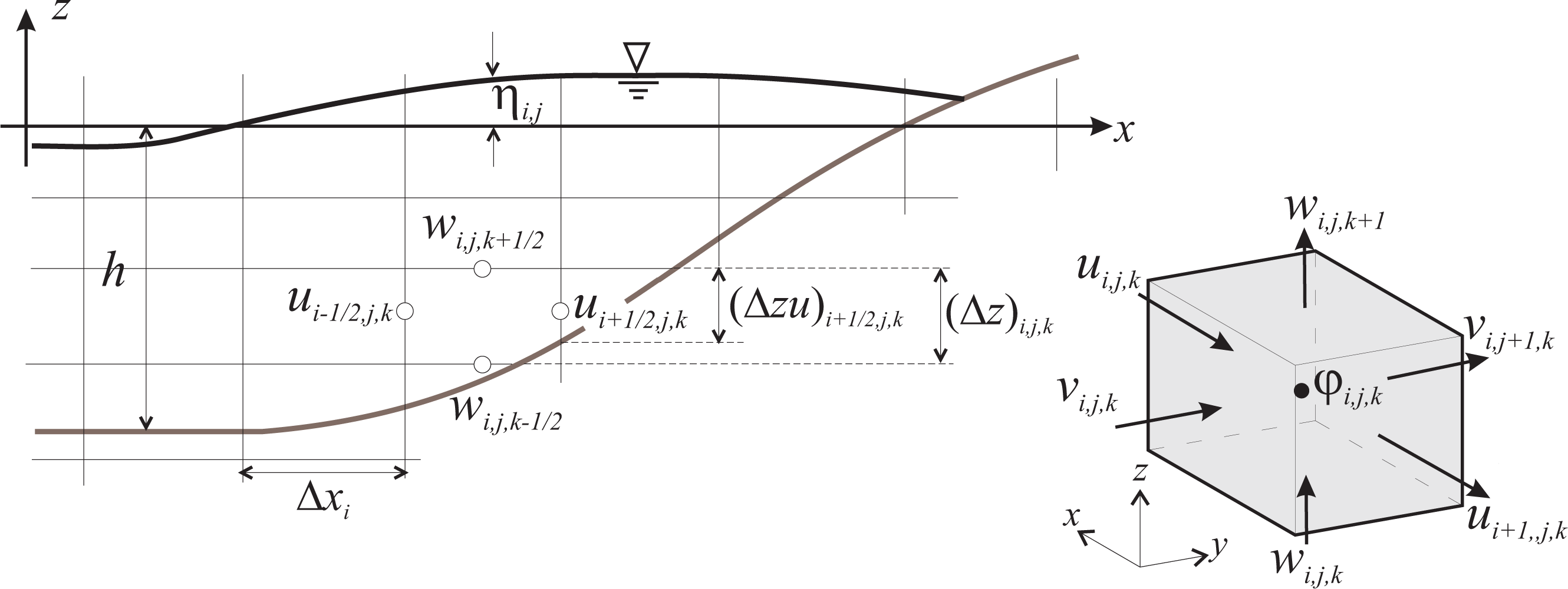
When vegetation is present in the flow, the bottom stress in terms of the shear law is defined, in the x and y directions, as:

$${\tau }_x^b={\rho }_0{C}_D^{b}U\sqrt{U^2+V^2},$$

(6)

$${\tau }_y^b={\rho }_0{C}_D^{b}V\sqrt{U^2+V^2},$$

(7)

where $C_D^b$ is the bottom stress coefficient, which is a function of the bottom relative roughness k_s/h and the Reynolds number, (Re), as:

$$C_D^b=\{\begin{array}{ll}0.2044{\left\{\text{log}\left[1.72/\text{Re}+{\left(k_s/14.8h\right)}^{1.11}\right]\right\}}^2\hfill & \text{if}\hspace{0.17em}\hspace{0.17em}{k}_s/h<\mathrm{0.2.}\hfill \\ 1.56x{10}^{-2}{\left(k_s/h\right)}^{\frac{1}{3}}\hfill & \text{if}\hspace{0.17em}\hspace{0.17em}\hspace{0.17em}\hspace{0.17em}{k}_s/h\ge \mathrm{0.2.}\hfill \end{array}$$

(8)

Equation (8) is taken from Arega and Sanders [20]. If the bottom roughness, k_s, is known in terms of the Manning coefficient, n, the following definition is used:

$$k_s=0.3048{(n/0.031)}^6.$$

(9)

When vegetation is not present, the bottom stress coefficient $C_D^b$ is calculated as follows:

$$C_D^b=\left[\frac{1}{\kappa }\text{ln}\left(\frac{h+z_b}{k_s}\right)\right].$$

(10)

The shear stress caused by the presence of vegetation is given by [39]:

$${\tau }_x^v=\frac{1}{2}{\rho }_0{C}_D^v{A}_{x}MU\sqrt{U^2+V^2},$$

(11)

$${\tau }_y^v=\frac{1}{2}{\rho }_0{C}_D^v{A}_{y}MV\sqrt{U^2+V^2},$$

(12)

where $C_D^v$ is the vegetation stress coefficient; M is the vegetation density per unit area (m⁻²); and A_x and A_y are the effective plant blocking areas (m²) in the x and y directions, respectively. For a two-dimensional simulation, the blocking areas of a plant are approximated by the product of the undeflected plant height (h_p) and the effective width of the plant (W_e). This effective area is the rectangular equivalent area of the foliage mass, where small stems are ignored, because they are not considered part of the mean mass of the foliage. For a three-dimensional simulation, the blocking areas correspond to the effective plant blocking areas of each single element of the mesh array. With dense foliage, for example, the blocking areas of each single element are near A_x = ΔxΔz and A_y = ΔyΔz, where Δx and Δy are the horizontal cell sizes and Δz is the vertical layer thickness.

Equations (11) and (12) are related to the drag caused by plants [40]. Freeman [10] defined a set of equations to calculate the drag forces. These equations relate the shear velocity to the mean velocity, as follows:

$$\frac{U^{*}}{U}=\frac{\sqrt{g{R}_{hx}S}}{U}={\left(\frac{{\tau }_x^v}{{\rho }_0{U}^2}\right)}^{\frac{1}{2}}={\left(\frac{A_{x}M{C}_D^v}{2}\right)}^{\frac{1}{2}},$$

(13)

$$\frac{V^{*}}{V}=\frac{\sqrt{g{R}_{hy}S}}{V}={\left(\frac{{\tau }_y^v}{{\rho }_0{V}^2}\right)}^{\frac{1}{2}}={\left(\frac{A_{y}M{C}_D^v}{2}\right)}^{\frac{1}{2}},$$

(14)

where U^* is the shear velocity (m/s); R_hx and R_hy are the cell hydraulic radii in the x and y directions, respectively (m); and S is the slope (dimensionless).

Relating Equations (13) and (14) with Equations (11) and (12), respectively, yields:

$${\tau }_x^v=\frac{A_{x}M{C}_D^v}{2}{\rho }_{0}U\sqrt{U^2+V^2}={\left(\frac{U^{*}}{U}\right)}^2{\rho }_{0}U\sqrt{U^2+V^2},$$

(15)

$${\tau }_y^v=\frac{A_{y}M{C}_D^v}{2}{\rho }_{0}V\sqrt{U^2+V^2}={\left(\frac{V^{*}}{V}\right)}^2{\rho }_{0}V\sqrt{U^2+V^2}.$$

(16)

For flexible plants, the equation that relates the shear velocity and the mean velocity is [10]:

$$\frac{U^{*}}{U}=0.183{\left(\frac{E_s{A}_s}{\rho A_x{U}^{*2}}\right)}^{0.183}{\left(\frac{h_p}{h}\right)}^{0.243}{\left(M{A}_x\right)}^{0.273}{\left(\frac{\nu }{U^{*}{R}_{hx}}\right)}^{0.115},$$

(17)

where E_s is the plant flexibility (N/m²); and A_s is the stem blocking area (m²). In this case, Re is a function of the cell hydraulic radius (R_hx) and the cell velocity. Equation (17) is to be applied only for submerged flow, where the water depth is greater than 0.8-times the undeflected plant height [10]. For the vertical velocity component V, Equation (17) is analogous.

The plant characteristics h_p, A_x, A_y and A_s are the initial characteristics of the plants without the effects of flow distortion.

3. Numerical Model

In order to achieve good accuracy in the velocity calculation and to consider different vegetation heights, a multilayer model-based approach is used. Figure 1 depicts how the numerical model considers different vegetation heights within the water.

A spatial mesh, which consists of rectangular cells with horizontal sizes Δx and Δy and height Δz is used. Scalars are located at the center of cells, and velocity components are shifted to the center of cell edges. Each cell’s center position is described using i, j and k. The computational mesh is shown in Figure 2.

The numerical model is based on a second-order finite difference formulation. The time accuracy is also second-order, and the solution method is an adaptation of the semi-implicit Eulerian-Lagrangian scheme proposed by Casulli and Cheng [41]. This method treats the advection and diffusion terms differently. The solution of the advection terms is given by a Lagrangian formulation through the characteristic method, and the solution of the diffusion terms is given by an Eulerian formulation through the Adams–Bashforth scheme.

In the Lagrangian scheme of the advection terms, the total derivative for velocity is used, providing a low numerical diffusivity and an unrestricted Courant condition. Advection accuracy is also known to be vital for realistic prediction of recirculating flows and must be second-order. These terms are treated explicitly, and to maintain second-order temporal accuracy, a second-order interpolation formula has been chosen. In the one-dimensional case, the interpolation gives:

$$U_{i-a}^n=(1-p^2)U_i^n+(0.5p^2+0.5p)U_{i-1}^n+(0.5p^2-0.5p)U_{i+1}^n,$$

(18)

where p is the Courant number.

Vertical diffusion is treated semi-implicitly with first-order accuracy to enhance stability and, hence, to get an overall robust scheme. Then, discretization of Equations (1) and (2) is written by a compact matrix form as:

$${\mathbf{A}}_{i+1/2,j}^n{\mathbf{U}}_{i+1/2,j}^{n+1}={\mathbf{G}}_{i+1/2,j}^n-g\frac{\mathrm{\Delta }t}{\mathrm{\Delta }x}\left({\eta }_{i+1,j}^{n+1}-{\eta }_{i,j}^{n+1}\right)\mathbf{\Delta }\mathbf{Z}{\eta }_{i+1/2,j}^n,$$

(19)

$${\mathbf{A}}_{i,j+1/2}^n{\mathbf{V}}_{i,j+1/2}^{n+1}={\mathbf{G}}_{i,j+1/2}^n-g\frac{\mathrm{\Delta }t}{\mathrm{\Delta }y}\left({\eta }_{i,j+1}^{n+1}-{\eta }_{i,j}^{n+1}\right)\mathbf{\Delta }\mathbf{Z}{\eta }_{i,j+1/2}^n,$$

(20)

where U, V, ΔZ and G are:

$$\begin{array}{c}{\mathbf{U}}_{i+1/2,j}^{n+1}=\left[\begin{array}{c}{U}_{i+1/2,j,M}^{n+1}\\ U_{i+1/2,j,M-1}^{n+1}\\ U_{i+1/2,j,M-2}^{n+1}\\ ⋮\\ U_{i+1/2,j,m}^{n+1}\end{array}\right],\hspace{0.17em}\hspace{0.17em}{\mathbf{V}}_{i,j+1/2}^{n+1}=\left[\begin{array}{c}{V}_{i,j+1/2,M}^{n+1}\\ V_{i,j+1/2,M-1}^{n+1}\\ V_{i,j+1/2,M-2}^{n+1}\\ ⋮\\ V_{i,j+1/2,m}^{n+1}\end{array}\right],\hspace{0.17em}\hspace{0.17em}\mathbf{\Delta }\mathbf{Z}=\left[\begin{array}{c}\mathrm{\Delta }{z}_M\\ \mathrm{\Delta }{z}_{M-1}\\ \mathrm{\Delta }{z}_{M-2}\\ ⋮\\ \mathrm{\Delta }{z}_m\end{array}\right],\\ {\mathbf{G}}_{i+1/2,j}^n=\left[\begin{array}{c}\mathrm{\Delta }{z}_{M}F{U}_{i+1/2,j,M}^n\\ \mathrm{\Delta }{z}_{M-1}F{U}_{i+1/2,j,M-1}^n\\ \mathrm{\Delta }{z}_{M-2}F{U}_{i+1/2,j,M-2}^n\\ ⋮\\ \mathrm{\Delta }{z}_{m}F{U}_{i+1/2,j,m}^n-\mathrm{\Delta }t{\tau }_x^b\end{array}\right],\hspace{0.17em}\hspace{0.17em}{\mathbf{G}}_{i,j+1/2}^n=\left[\begin{array}{c}\mathrm{\Delta }{z}_{M}F{V}_{i,j+1/2,M}^n\\ \mathrm{\Delta }{z}_{M-1}F{V}_{i,j+1/2,M-1}^n\\ \mathrm{\Delta }{z}_{M-2}F{V}_{i,j+1/2,M-2}^n\\ ⋮\\ \mathrm{\Delta }{z}_{m}F{V}_{i,j+1/2,m}^n-\mathrm{\Delta }t{\tau }_y^b\end{array}\right],\end{array}$$

and A is defined as:

$$\begin{array}{l}{\mathbf{A}}_{i+1/2,j}^n={\mathbf{A}}_{i,j+1/2}^n=\\ \left[\begin{array}{cccc}\mathrm{\Delta }{z}_M+\frac{{\nu }_{TV\hspace{0.17em}M-1/2}\mathrm{\Delta }t}{\mathrm{\Delta }{z}_{M-1/2}}& \frac{-{\nu }_{TV\hspace{0.17em}M-1/2}\mathrm{\Delta }t}{\mathrm{\Delta }{z}_{M-1/2}}& \cdots & 0\\ \frac{-{\nu }_{TV\hspace{0.17em}M-1/2}\mathrm{\Delta }t}{\mathrm{\Delta }{z}_{M-1/2}}& \mathrm{\Delta }{z}_{M-1}+\frac{{\nu }_{TV\hspace{0.17em}M-1/2}\mathrm{\Delta }t}{\mathrm{\Delta }{z}_{M-1/2}}+\frac{{\nu }_{TV\hspace{0.17em}M-3/2}\mathrm{\Delta }t}{\mathrm{\Delta }{z}_{M-3/2}}& \frac{-{\nu }_{TV\hspace{0.17em}M-3/2}\mathrm{\Delta }t}{\mathrm{\Delta }{z}_{M-3/2}}& \\ ⋮& ⋮& ⋮& \\ 0& & \frac{-{\nu }_{TV\hspace{0.17em}m+1/2}\mathrm{\Delta }t}{\mathrm{\Delta }{z}_{m+1/2}}& \mathrm{\Delta }{z}_m+\frac{{\nu }_{TV\hspace{0.17em}m+1/2}\mathrm{\Delta }t}{\mathrm{\Delta }{z}_{m+1/2}}\end{array}\right],\end{array}$$

where m and M denote the k-index of the bottom and the top finite difference stencil, respectively. The finite difference operator F for U (analogous for V) is defined as:

$$\begin{array}{ll}F{U}_{i+1/2,j,k}^n\hfill & =U_{i+1/2-a,j-b,k-d}^n\hfill \\ \hfill & +{\nu }_{TH}\mathrm{\Delta }t(\frac{U_{i+1/2-a+1,j-b,k-d}^n-2U_{i+1/2-a,j-b,k-d}^n+U_{i+1/2-a-1,j-b,k-d}^n}{\mathrm{\Delta }{x}^2}\hfill \\ \hfill & +\frac{U_{i+1/2-a,j-b+1,k-d}^n-2U_{i+1/2-a,j,-b,k-d}^n+U_{i+1/2-a,j-b-1,k-d}^n}{\mathrm{\Delta }{y}^2}).\hfill \end{array}$$

Equations (19) and (20) are linear tridiagonal systems, which are coupled to the water surface elevation ηⁿ⁺¹ at time tⁿ⁺¹. In order to calculate ${\eta }_{i,j}^{n+1}$ and for numerical stability, the new velocity field must satisfy for each i, j the following equation, which is the matrix form of Equation (4):

$$\begin{array}{ll}{\eta }_{i,j}^{n+1}\hfill & ={\eta }_{i,j}^n-\frac{\mathrm{\Delta }t}{\mathrm{\Delta }x}\left[{\left(\mathbf{\Delta }{\mathbf{z}}_{i+1/2,j}\right)}^T{\mathbf{U}}_{i+1/2,j}^{n+1}-{\left(\mathbf{\Delta }{\mathbf{z}}_{i-1/2,j}\right)}^T{\mathbf{U}}_{i-1/2,j}^{n+1}\right]\hfill \\ \hfill & -\frac{\mathrm{\Delta }t}{\mathrm{\Delta }y}\left[{\left(\mathbf{\Delta }{\mathbf{z}}_{i,j+1/2}\right)}^T{\mathbf{V}}_{i,j+1/2}^{n+1}-{\left(\mathbf{\Delta }{\mathbf{z}}_{i,j-1/2}\right)}^T{\mathbf{V}}_{i,j-1/2}^{n+1}\right].\hfill \end{array}$$

(21)

Equations (19) and (20) constitute a linear system with unknowns ${\mathbf{U}}_{i+1/2,j}^{n+1}$, ${\mathbf{V}}_{i,j+1/2}^{n+1}$ and ${\eta }_{i,j}^{n+1}$ over the entire computational mesh. To be solved and for computational convenience, this system is reduced by substituting Equations (19) and (20) in (21), in which ${\eta }_{i,j}^{n+1}$ are the only unknowns.

The present numerical model has been validated and applied for different cases of study. The cases of study have been simple, controlled experiments and real free surface flows in rivers, lakes, lagoons, estuaries and nearshore flows. The numerical model has been validated by Ramírez-León et al. [42] to study the dispersion of thermal and saline plumes in lakes and estuarine water bodies. Ramírez-León et al. [42] compared the results against other similar models, achieving good agreement. The thermal plume dispersion of the Laguna Verde Nuclear Power Plant, located in Mexico, was also studied by using the present numerical model, with the results shown in [43]. Rodríguez et al. [44] applied the numerical model to predict two types of island wakes, and the results showed good agreement with the experiments. More details about the present numerical model and other applications are given in [45–47].

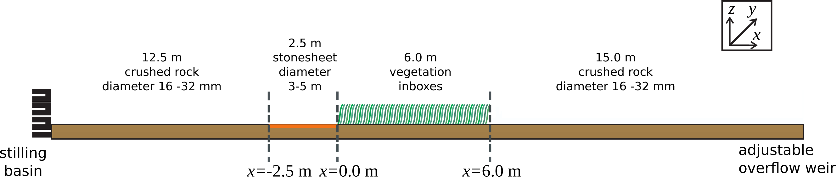
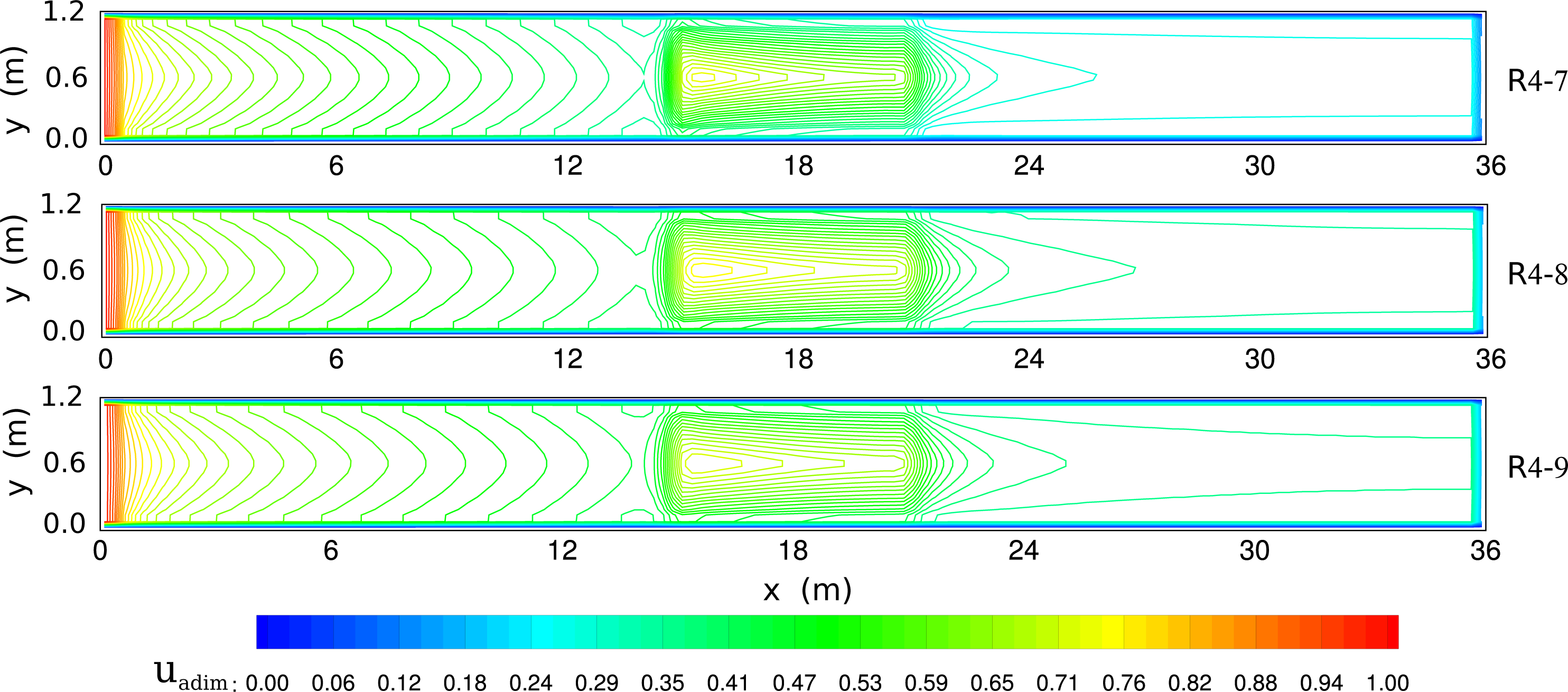
4. Numerical Simulations and Discussion

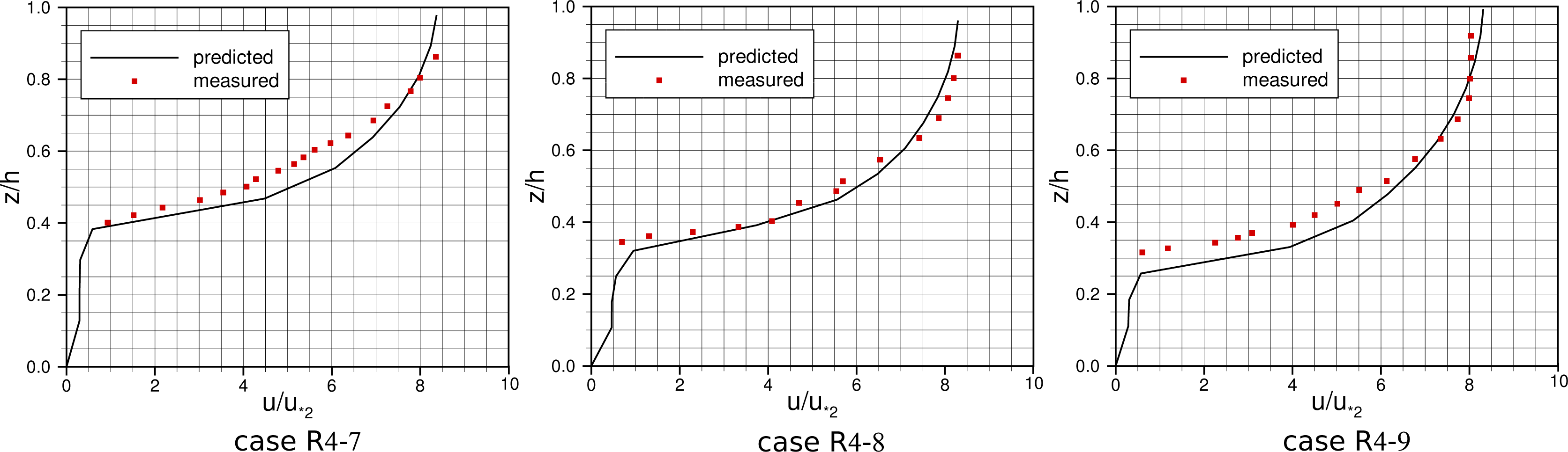
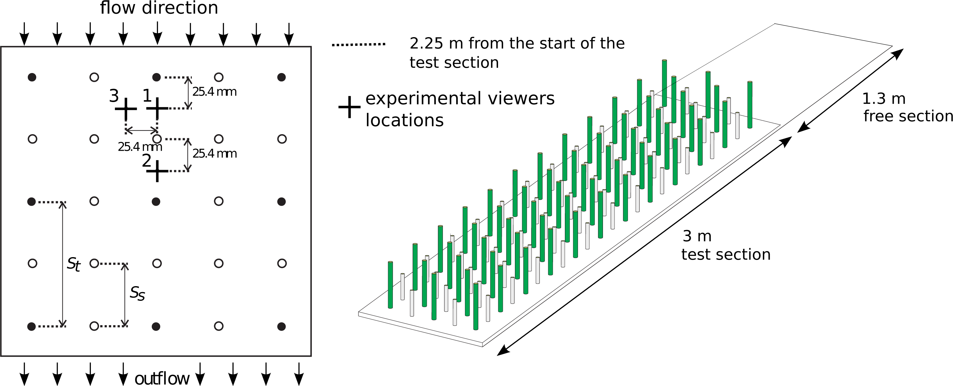
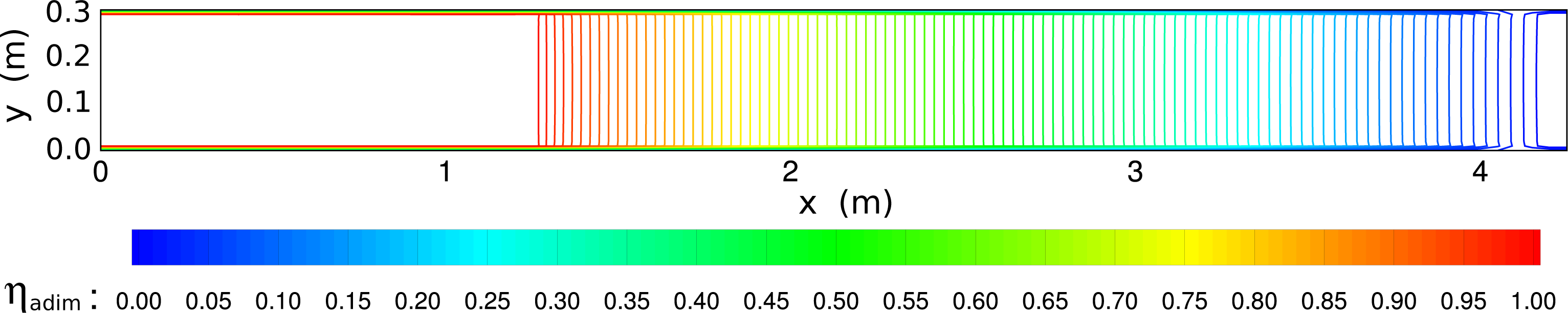
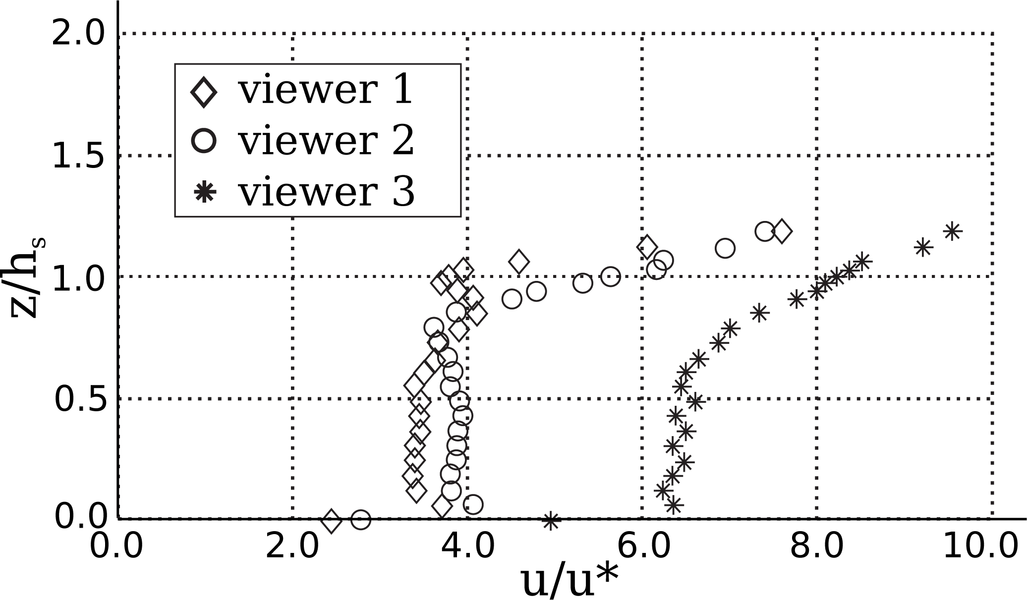
4.1. Channel with Submerged Vegetation

Validation of our results was carried out by comparing them to measurements presented by Järvelä [48]. Järvelä analyzed the behavior of velocity profiles above a vegetated layer over a number of different experiments, three of which are numerically reproduced here for comparison. The numerical simulations were conducted for a channel 36 m long and 1.1 m wide. The plants covered a 6-m section at the center of the channel. The vegetation density was, on average, 12, 000 stems/m². Sections 15 m long before and after the vegetation area were covered with a 0.10 m-thick layer of crushed rock (rock diameter: 16–32 mm), with the exception of the 2.5-m length directly before the vegetation area. This section was covered with smoother crushed rock (diameter: 3–5 mm). Figure 3 shows a diagram of the experimental setup, and

Table 1. Experimental setup (taken from Järvelä [48]).

Case	Q (l/s)	h (m)	U0 (m/s)	Re	Fr	Se	u*2 (m/s)	hp (m)	f
R4-7	100	0.4950	0.1836	60,606	0.083	0.0006	0.0416	0.220	0.68
R4-8	100	0.7065	0.1287	60,606	0.049	0.0002	0.027	0.260	0.50
R4-9	143	0.7037	0.1847	86,667	0.070	0.0003	0.0384	0.215	0.44

summarizes the initial conditions of the three selected cases.

In Table 1, Q is the discharge, U₀ is the inflow velocity, Re = U₀h/ν, $\text{Fr}=U_0/\sqrt{gh}$, S_e is the energy slope, h_p is the undeflected vegetation height and u_*2 is the shear velocity given by:

$$u_{*2}=\sqrt{g(h-h_p)S_e}.$$

(22)

The measured and predicted velocity profiles were compared at three different longitudinal locations for all cases: at x = 3.5, 3.65 and 3.8; and y = 0.4. These profiles are located above the vegetated layer.

For the three numerical simulations, a rectangular grid of 144 × 22 points was implemented, with constant mesh sizes Δx and Δy. The vegetation was located in the zone shown in Figure 3, which covers five vertical layers for all cases. The time step was 1 × 10⁻³ s. In order to achieve good accuracy in the calculation of vertical velocity variations, multiple layers with different heights were used for each case: 12 layers for case R4-7; and 14 layers for cases R4-8 and R4-9. The initial velocity components and the free surface elevation were zero. At the inflow section, a parabolic U velocity profile was imposed, where the mean velocity was the inflow velocity U₀. An appropriate bottom roughness (k_s) was imposed to characterize the thick layer of crushed rock at the bottom of the channel before and after the vegetation zone.

Figures 4 and 9 show the results from the present numerical model. In general, the flow pattern is similar for the three cases; the flow is steady, parallel and symmetric with respect to the mid-longitudinal axis. The U and V velocity fields at the free surface layer in Figures 4 and 5 show that the flow velocity increases above the vegetated zone. Within the vegetation, the flow velocity components significantly decrease, as can be seen in Figures 6 and 7, where the velocity fields in the fourth layer from the bottom are shown. This fourth layer is found just below the top of the plants and for the cases R4-7, R4-8 and R4-9 is 0.176 m, 0.208 m and 0.215 m from the bottom, respectively.

An analogy can be observed from the predictions. The flow pattern predicted by the numerical model over the vegetation presents the typical characteristics of flow over a rectangular broad-crested weir, where the flow depth decreases and the velocity magnitude increases (see Figures 8 and 9). Contours of the velocity field and free surface variations are difficult to find in previous works, for describing an instantaneous flow pattern, in channel flows with the presence of submerged vegetation.

The vertical distribution of the U velocity component shown in Figure 9 allows us to observe that in the upper layer, above the vegetation, the velocity gradually decreases from the surface to the vegetation zone. This is due to the effects of the vegetation and bottom shear stresses. As shown in Figure 9, the streamlines follow a horizontal direction from the channel inlet to the vegetation region. When they reach the vegetation region, the streamlines suffer a contraction in the free surface layer. After the vegetation region, as the channel section is expanded, the streamlines recover the trajectory that they had before the vegetation region.

Figure 10 compares the averaged velocity profiles from Järvelä [48] and the predicted profiles obtained from the current numerical model. In general, the predictions have good agreement with the experimental measurements.

The corresponding correlation coefficients yield R = 0.9827 for case R4-7, R = 0.9935 for case R4-8 and R = 0.9947 for case R4-9. Järvelä reported that the disturbance of the acoustic pulse caused by vegetation elements entering the ADV-sampling volume limited measurements close to the vegetation in some test runs. However, the predictions obtained from the numerical simulations allow us to characterize flow patterns, even within the vegetated layer.

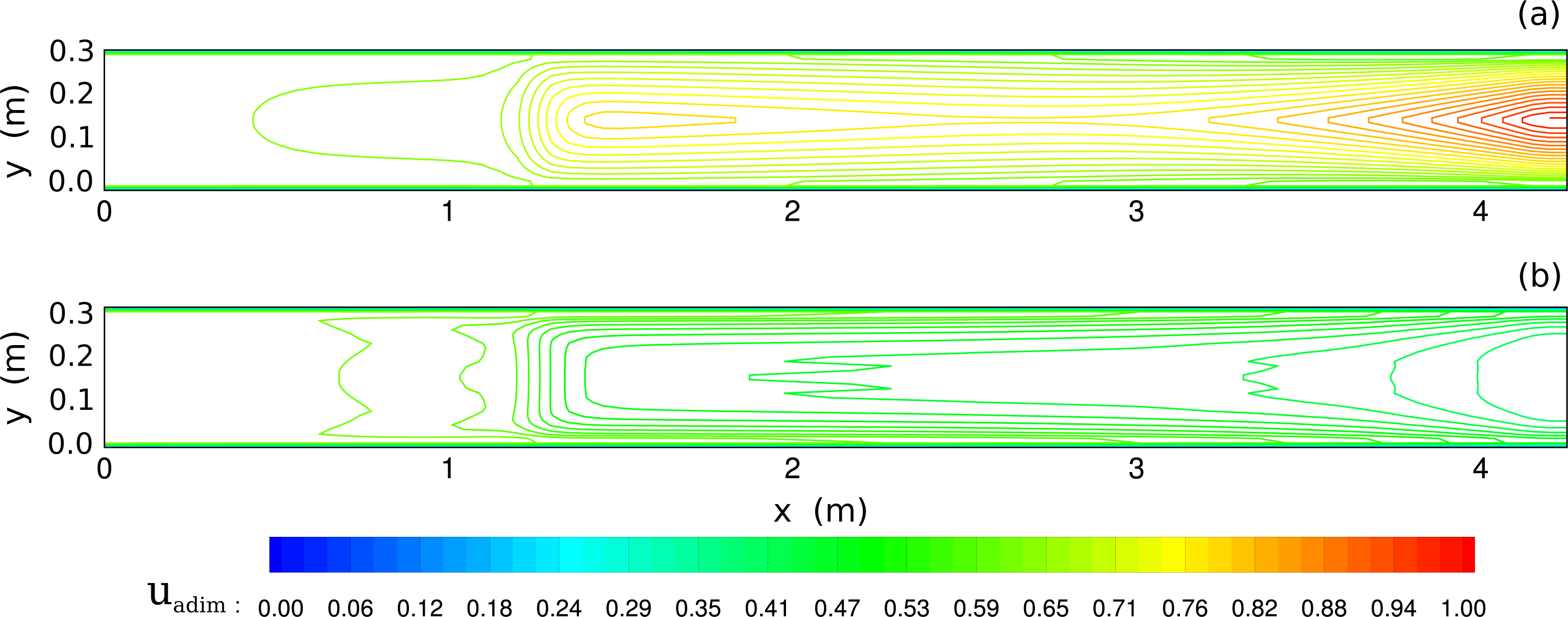
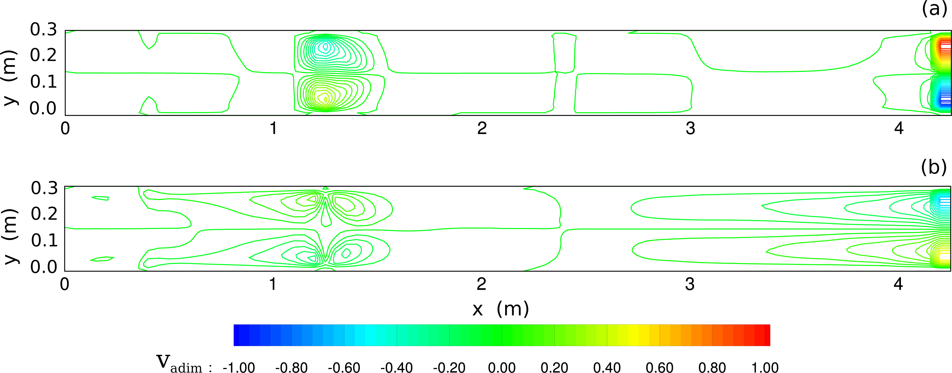
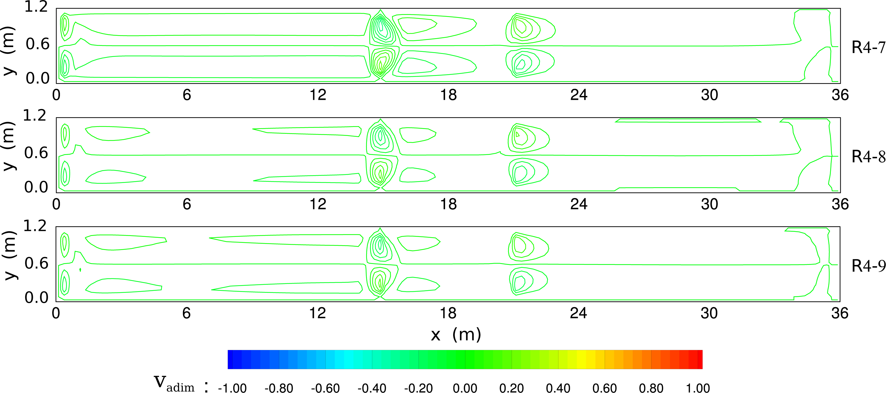
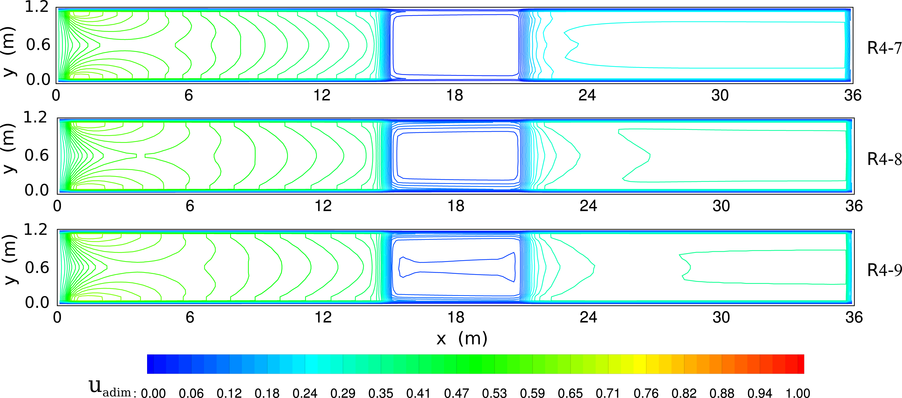
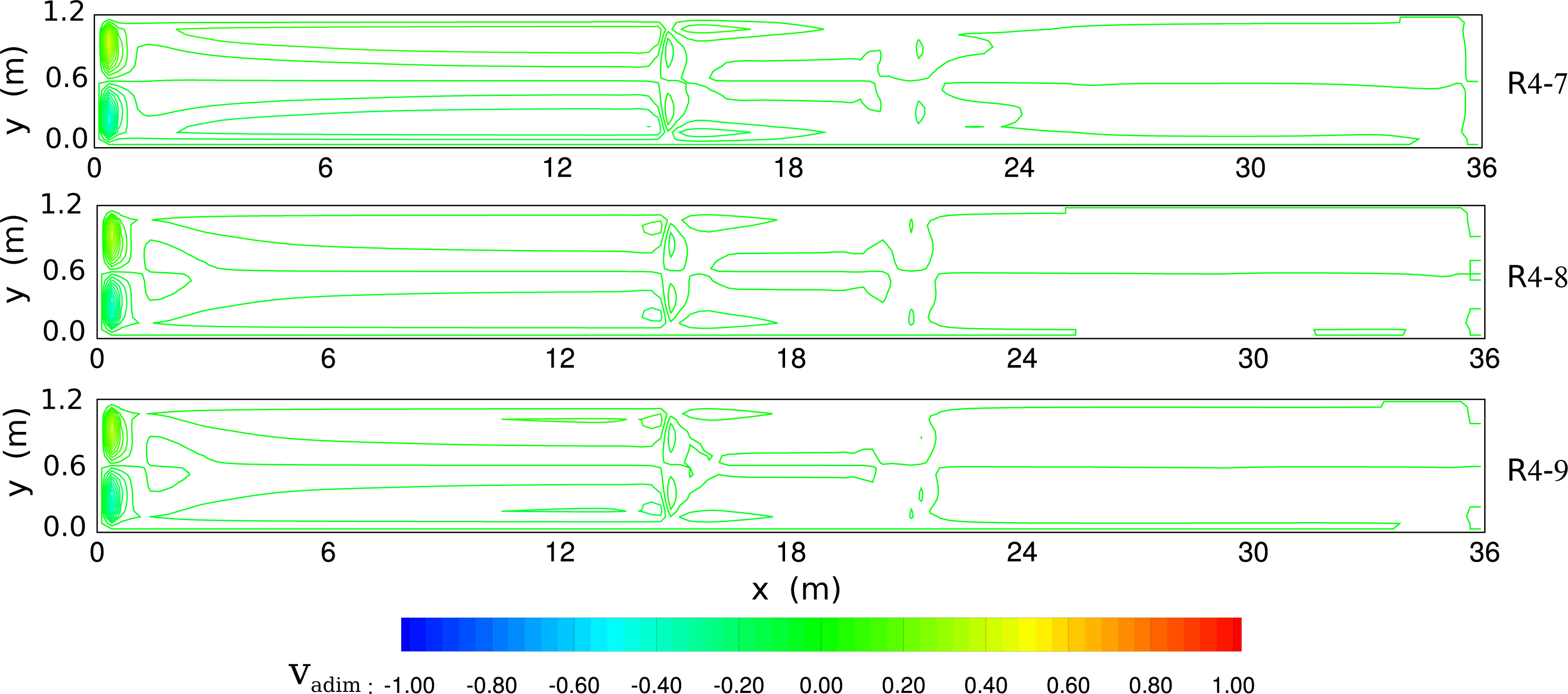
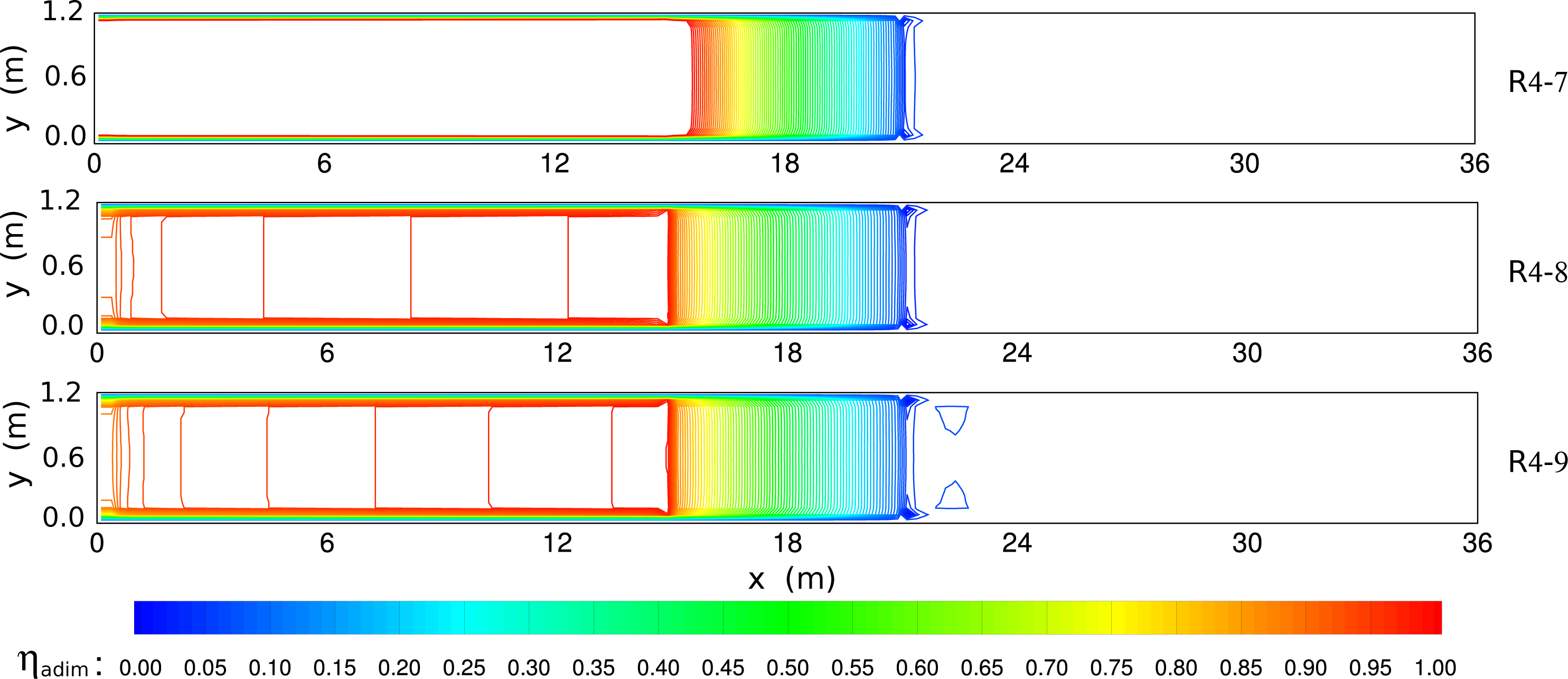
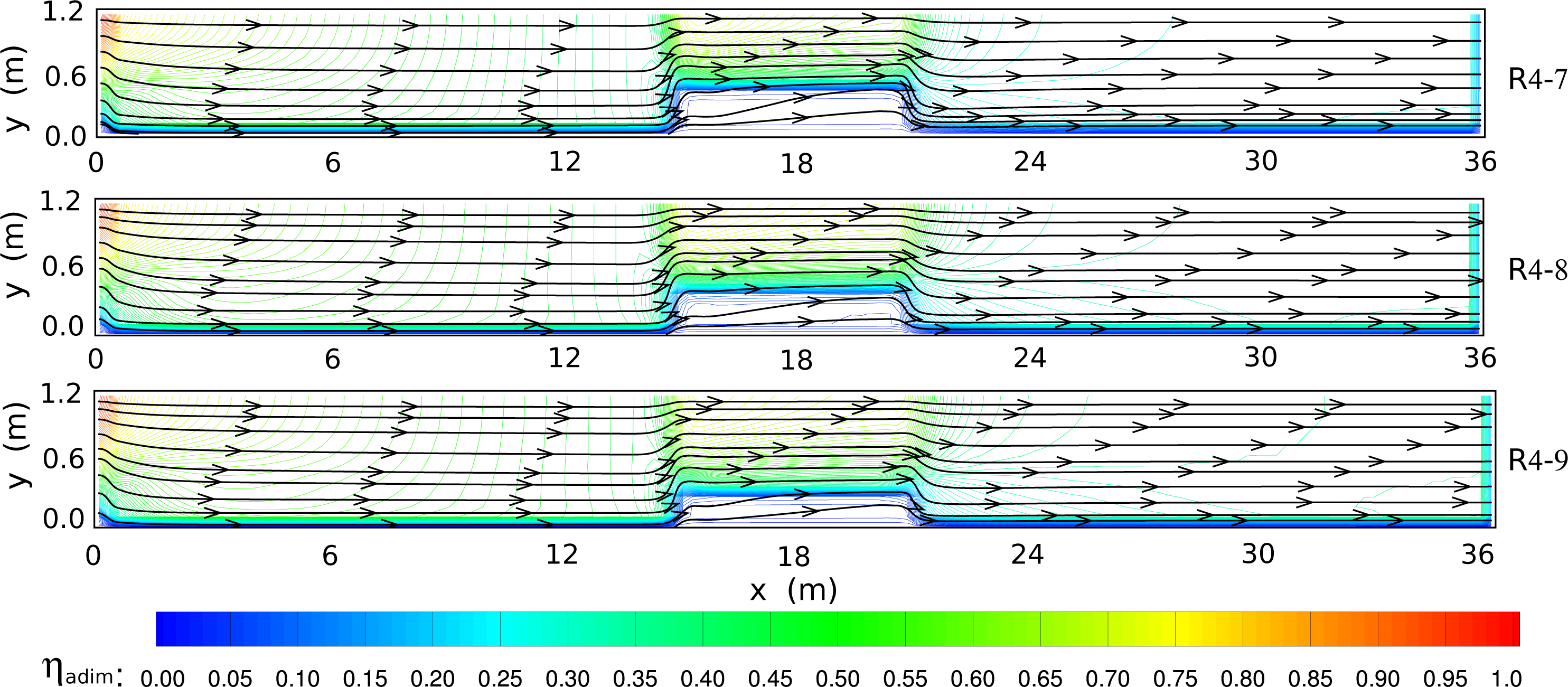
4.2. Channel with Submerged and Emergent Vegetation

To show the ability of the present turbulence model to reproduce the flow mechanisms within the vegetation region, we carried out numerical simulations by considering submerged and emergent vegetation. For this purpose, the experiment of Liu [49] was reproduced numerically for comparison. Liu analyzed velocity profiles for seven cases within a layer of rigid vegetation represented by dowels. Four of these cases were configured with emergent and submerged vegetation by changing the dowel distributions. The experiment consisting of a linear distribution of emergent and submerged dowels was also reproduced by numerical simulation.

Liu’s experiment was conducted in a channel 4.3 m long and 0.3 m wide, with a depth of 0.1046 m, maintained at a constant slope of 0.003. The 3.0 m-long vegetation test section covered the entire width and was located 1.3 m from the entrance of the flume. The vegetation was simulated by 6.35 mm diameter (d), acrylic dowels, cut to lengths of 76 mm for short dowels and 152 mm for large dowels. The discharge was 0.0114 m³/s. The spacing was determined by non-dimensional parameters; S_s/d = 8 and S_t/d = 16 for short and tall dowels, respectively, arranged in a linear pattern. Instantaneous longitudinal velocities were taken 2.25 m downstream of the start of the test section, using a laser Doppler velocimeter (LDV). Measurement locations are shown in Figure 11, where the LDV was located 4d downstream from a large dowel (Viewer 1) and 4d downstream from a short dowel (Viewer 2), and a single measurement location was selected in a point where there are no dowels, either upstream or downstream (Viewer 3).

For the numerical simulation, a grid of rectangular elements, 86 × 32 points, with constant mesh sizes Δx and Δy and nine vertical layers of constant height were used. The short dowels covered six vertical layers in height, while the tall dowels covered all layers. Since the diameter and roughness of short and tall dowels are the same, a variable vegetation density was imposed in the vertical direction to characterize the height difference between them. The effective dowel blocking areas were considered in A_x and A_y to calculate the shear stress caused by vegetation (Equations (15) and (16)). The initial velocity components and free surface elevation were zero. The time step was 1 × 10⁻⁵ s. A constant linear velocity profile was imposed at the inflow section, where the mean inflow velocity was obtained from a discharge of 0.0114 m³/s. Velocity values were recorded 2.25 m from the beginning of the test section at the center of the channel, for comparison to measurements.

Figures 12 and 14 illustrate the velocity field at the free surface layer and at 0.038 m from the bottom, which is the mid-height of the short dowels. The flow pattern is symmetric with respect to the longitudinal centerline, as can be observed in Figures 12 and 13. When the flow reaches the vegetation region at 1.3 m from the beginning of the channel, the effect of vegetation is evident. At the layer where the effective dowel blocking area is composed by both large and short dowels (see Figures 12b and 13b), the flow suffers an important deceleration, compared with the flow at the surface layer, where the blocking area is constituted only by large dowels (see Figure 12a and 13a). The effects of vegetation on flow are also visible from the behavior of the free surface elevation (see Figure 14). The free surface elevation is not perturbed through the non-vegetated flow region, where it maintains a constant value. Within the vegetation region, the free surface elevation slowly decreases up to reach the channel outlet.

The vertical velocity profile predicted by the numerical simulation was compared against measurements. Figure 15 shows the U velocity measurements of Liu [49], in Locations 1, 2 and 3, as defined in Figure 11. Figure 16 shows a comparison between the averaged-profile generated from the U velocity measurements taken by Liu (Figure 15) and the predicted U velocity profile. The dimensionless velocity values were obtained from the shear velocity as follows:

$$u^{*}=\sqrt{gh{S}_e}$$

(23)

From Figure 16, a correlation coefficient R = 0.9286 is obtained. As can be observed, the predictions show poor agreement compared with measurements. The predictions fail to characterize the near uniform velocity within the densest region of the vegetation array. They also miss the inflection near z/h_s = 1.0.

5. Conclusions

This work presents a numerical model based on the Reynolds-averaged Navier–Stokes equations for shallow water flows in the presence of vegetation. A mixing-length model is used to characterize turbulence.

The multilayer approach allows the calculation of the vertical velocity profile from the bottom to the free surface at any location and any time, which is not possible by using logarithmic law-based analytical models and/or 2D numerical models.

The predictions obtained with the present numerical model were compared against experimental measurements found in the literature. The comparisons between predicted velocity profiles and experimental measurements show some limitations of the mixing-length model used, particularly within the vegetated region. When the flow presents a free surface layer, the case with submerged vegetation, the numerical model reproduces correctly the flow mechanisms in this layer. On the other hand, when the flow is totally covered by vegetation, the case with emergent and submerged vegetation, the comparisons between predictions and measurements show poor agreement.

There are definite limitations in the present turbulence model formulation. The main technical contribution of the manuscript must be Equation (5), which defines the turbulent eddy viscosity. However, the turbulent eddy viscosity in this equation is not a function of vegetation presence or absence, and the formulation proposed has been validated for only non-vegetated flows. Therefore, the turbulent eddy viscosity is not sufficiently validated in the vegetated region. It is likely that the turbulent eddy viscosity increases within vegetated areas, because of the high frequency phenomena. Additional eddies and turbulence are generated by the individual plants that are not explicitly represented in the model. It could be expected that there will generally be a mismatch between observed and predicted velocity within vegetated zones, because of the inaccuracy of the turbulent eddy viscosity, just as is shown in Figure 16. More additional work on the turbulence model formulation and validation must be accomplished and can be the subject of future work.

References

1. Newson, M.D. River Conservation and Catchment Management, Conservation and Management; Wiley: Chichester, UK, 1992; pp. 385–396. [Google Scholar]
2. Ward, J.; Tockner, K.; Uehlinger, U.; Malard, F. Understanding natural patterns and processes in river corridors as the basis for effective river restoration. Regul. Rivers Res. Manag 2001, 17, 311–323. [Google Scholar]
3. Nepf, H.; Vivoni, E. Flow structure in depth-limited vegetated flow. J. Geophys. Res 2000, 105, 28547–28557. [Google Scholar]
4. Tsujimoto, T. Fluvial processes in streams with vegetation. J. Hydraul. Res 1999, 37, 789–803. [Google Scholar]
5. Smart, G.M.; Duncan, M.J.; Walsh, J.M. Relatively rough flow resistance equations. J. Hydraul. Eng 2002, 128, 568–578. [Google Scholar]
6. Nikora, V.; Koll, K.; McEwan, I.; McLean, S.; Dittrich, A. Velocity distribution in the roughness layer of rough bed flows. J. Hydraul. Eng 2004, 130, 1036–1042. [Google Scholar]
7. Ghisalberti, M. Obstructed shear flows: Similarities across systems and scales. J. Fluid Mech 2009, 641, 51–61. [Google Scholar]
8. Cheng, N.S. Representative roughness height of submerged vegetation. Water Resour. Res 2011, 47. [Google Scholar] [CrossRef]
9. Nepf, H. Flow and transport in regions with aquatic vegetation. Annu. Rev. Fluid Mech 2012, 44, 123–142. [Google Scholar]
10. Freeman, G.E.; Rahmeyer, W.J.; Copeland, R.R. Determination of Resistance Due to Shrubs and Woody Vegetation; Technical report; U.S. Army Corps of Engineers; Coastal and Hydraulics Laboratory: Washington, DC, USA, 2000. [Google Scholar]
11. Järvelä, J. Determination of Flow Resistance of Vegetated Channel Banks and Floodplains. In River Flow; Zech, B., Bousmar, D., Eds.; Swets & Zeitlinger: Helsinki University of Technology, Finland, 2002. [Google Scholar]
12. Pechlivanidis, G.I.; Keramaris, E.; Pechlivandis, I.G.; Samaras, G.A. Measuring the turbulent characteristics in an open channel using the PIV method. Glob. NEST J 2012, 14, 378–385. [Google Scholar]
13. Stone, B.M.; Shen, H.T. Hydraulic Resistance of Flow in Channels with Cylindrical Roughness. J. Hydraul. Eng 2002, 128, 500–506. [Google Scholar]
14. Huthoff, F.; Augustijn, D.C.M.; Hulscher, S.J.M.H. Depth-Averaged Flow in Presence of Submerged Cylindrical Elements. In River Flow; Francis, T., Ed.; Taylor & Francis: London, UK, 2006; pp. 575–582. [Google Scholar]
15. Yen, B.C. Open Channel Flow Resistance. J. Hydraul. Eng 2002, 128, 20–39. [Google Scholar]
16. Feng, K.; Molz, F.J. A 2-D, diffusion based, wetland flow model. J. Hydrol 1997, 196, 230–250. [Google Scholar]
17. Fennema, R.J.; Neidrauer, C.J.; Johnson, R.A.; MacVicor, T.K.; Perkins, W.A.A. Computer Model to Simulate Natural Everglades Hydrology. In Everglades The Ecosystem and Its Restoration; St. Lucie Press: Florida, USA, 1994; pp. 249–289. [Google Scholar]
18. Lal-Wasantha, A.M. Performance comparison of overland flow algorithms. J. Hydraul. Division ASCE 1998, 124, 342–349. [Google Scholar]
19. Rowinski, P.M.; Kubrak, J. A mixing-length model for predicting vertical velocity distribution in flows through emergent vegetation. Hydrol. Sci. J 2002, 47, 893–904. [Google Scholar]
20. Arega, F.; Sanders, B.F. Dispersion Model for Tidal Wetlands. J. Hydraul. Eng 2004, 130, 739–754. [Google Scholar]
21. Fischer-Antze, T.; Stoesser, T.; Olsen, N.R.B. 3D numerical modeling of open-channel flow with submerged vegetation. J. Hydraul. Res 2001, 39, 303–310. [Google Scholar]
22. Choi, S.U.; Kang, H. Reynolds stress modeling of vegetated open-channel flows. J. Hydraul. Res 2004, 42, 3–11. [Google Scholar]
23. Yusuf, B.; Karim, O.A.; Osman, S.A. Numerical solution for open channel flow with submerged flexible vegetation. Int. J. Eng. Tech 2009, 61, 39–50. [Google Scholar]
24. Jahra, F.; Yamamoto, H.; Hasegawa, F.; Kawahara, Y. Turbulent Flow Structure in Meandering Vegetated Open Channel; Bundesanstalt für Wasserbau: Higashi-Hiroshima, Japan, 2010; pp. 153–161. [Google Scholar]
25. Gao, G.; Falconer, R.A.; Lin, B. Modeling open channel flows with vegetation using a three-dimensional model. J. Water Res. Prot 2011, 3, 114–119. [Google Scholar]
26. Shimizu, Y.; Tsujimoto, T. Numerical analysis of turbulent open-channel flow over a vegetation layer using a k-ε turbulence model. J. Hydrosci. Hydraul. Eng 1994, 11, 57–67. [Google Scholar]
27. Lopez, F.; Garcia, M.H. Open-Channel Flow Through Simulated Vegetation: Turbulence Modeling and Sediment Transport. Wetlands; Technical Report; Wetlands Research Program technical report, WRP-CP-10; University of Illinois: Urbana IL, USA, 1997. [Google Scholar]
28. Neary, V.S. Numerical Solution of Fully Developed Flow with Vegetative Resistance. J. Eng. Mech. ASCE 2003, 129, 558–563. [Google Scholar]
29. Naot, D.; Nezu, I.; Nakagawa, H. Hydrodynamic Behavior of Partly Vegetated Open-Channels. J. Hydraul. Eng. ASCE 1996, 122, 625–633. [Google Scholar]
30. Alamatian, E.; Jaefarzadeh, M. Evaluation of turbulence models in the simulation of oblique standing shock waves in supercritical channel flows. Int. J. Civ. Eng 2012, 10, 61–71. [Google Scholar]
31. Akilli, H.; Akar, A.; Karakus, C. Flow characteristics of circular cylinders arranged side-by-side in shallow water. Flow Meas. Instrum 2004, 15, 187–197. [Google Scholar]
32. Fu, H.; Rockwell, D. Shallow flow past a cylinder: Transition phenomena at low Reynolds number. J. Fluid Mech 2005, 540, 75–97. [Google Scholar]
33. Fu, H.; Rockwell, D. Shallow flow past a cylinder: Control of the near wake. J. Fluid Mech 2005, 539, 1–24. [Google Scholar]
34. Sadeque, M.A.F.; Rajaratnam, N.; Loewen, M.R. Flow around cylinders in open channels. J. Eng. Mech 2008, 134, 60–71. [Google Scholar]
35. Sadeque, M.A.F.; Rajaratnam, N.; Loewen, M.R. Effects of bed roughness on flow around bed-mounted cylinders in open channels. J. Eng. Mech 2009, 135, 100–110. [Google Scholar]
36. Rodi, W.; Scheuerer, G. Scrutinizing the k-epsilon turbulence model under adverse pressure gradient conditions. J. Fluids Eng. Trans. ASME 1986, 108, 174–179. [Google Scholar]
37. Lam, C.K.G.; Bremhorst, K. A modified form of the k-epsilon model for predicting wall turbulence. ASME Trans. J. Fluids Eng 1981, 103, 456–460. [Google Scholar]
38. Stansby, P.K. A mixing-length model for shallow turbulent wakes. J. Fluid Mech 2003, 495, 369–384. [Google Scholar]
39. Perlin, A.; Moum, J.N.; Klymak, J.M.; Levine, M.D.; Boyd, T.; Kosro, P.M. A modified law-of-the-wall applied to oceanic bottom boundary layers. J. Geophys. Res 2005, 110. [Google Scholar] [CrossRef]
40. Kadlec, R.H. Overland flow in wetlands: Vegetation resistance. J. Hydraul. Eng 1990, 116, 691–706. [Google Scholar]
41. Casulli, V.; Cheng, R.T. Semi-implicit finite difference methods for three dimentional shallow water flow. Int. J. Numer. Methods Fluids 1992, 15, 629–648. [Google Scholar]
42. Ramírez-León, H.; Barrios-Piña, H.; Rodríguez-Cuevas, C.; Couder-Castañeda, C. Baroclinic mathematical modeling of fresh water plumes in the interaction river-sea. Int. J. Numer. Anal. Model 2005, 2, 1–14. [Google Scholar]
43. Ramírez-León, H.; Couder-Castañeda, C.; Herrera-Díaz, I.E.; Barrios-Piña, H. Modelación numérica de la descarga térmica de la Central Nucleo-eléctrica de Laguna Verde. Rev. Int. Mét. Num. Cálc. Dis. Ing 2010, 15, 185–211. [Google Scholar]
44. Rodríguez, C.; Serre, E.; Rey, C.; Ramírez, H. A numerical model for shallow-water flows: Dynamics of the eddy shedding. Wseas Trans. Environ. Dev 2005, 1, 280–287. [Google Scholar]
45. Ramírez-León, H.; Rodríguez-Cuevas, C.; Herrera Díaz, E. Multilayer hydrodinamic model and their application to sediment transport in estuaries. In Special Issue Shangai Conference, Current Trends in High Performance Computing and Its Applications; Springer-Verlag: Berlin, Germany, 2005; pp. 59–70. [Google Scholar]
46. Couder, C.; Ramírez, H.; Herrera, E. Numerical Modeling of Coupled Phenomena in Science and Enginering: Practical Use and Examples; Taylor & Francis: London, UK, 2008. [Google Scholar]
47. Herrera-Díaz, I.E.; Couder-Castañeda, C.; Ramírez-León, H. A case study of nearshore wave transformation processes along the coast of Mexico near the Laguna verde nuclear power plant using a fast simulation method. Model. Simul. Eng 2010, 1, 8–17. [Google Scholar]
48. Järvelä, J. Effect of submerged flexible vegetation on flow structure and resistance. J. Hydrol 2005, 307, 233–241. [Google Scholar]
49. Liu, D. Flow through Rigid Vegetation Hydrodynamics, Virginia Polytechnic Institute and State University, Blacksburg, VA, USA, 12 September 2008.
Figure 1. The multi-layer approach in the presence of vegetation. An example showing four layers and different plant heights.
Water 06 02084f1
Figure 2. Computational mesh and notation used, where φ represents a scalar quantity.
Water 06 02084f2
Figure 3. Experimental setup and definition of the coordinate axes (not to scale) (taken from Järvelä [48]).
Water 06 02084f3
Figure 4. U velocity component in the surface layer for the three cases. Where uadim = U/Umax.
Water 06 02084f4
Figure 5. V velocity component in the surface layer for the three cases. Where vadim = V/Vmax.
Water 06 02084f5
Figure 6. U velocity component at 0.176 m, 0.208 m and 0.215 m from the bottom, for the cases R4-7, R4-8 and R4-9, respectively. Where uadim = U/Umax.
Water 06 02084f6
Figure 7. V velocity component at 0.176 m, 0.208 m and 0.215 m from the bottom, for the cases R4-7, R4-8 and R4-9, respectively. Where vadim = V/Vmax.
Water 06 02084f7
Figure 8. Free surface elevation for the three cases. Where ηadim = (ηηmin)/(ηmaxηmin).
Water 06 02084f8
Figure 9. U velocity component and streamlines along the longitudinal mid-plane for the three cases, where uadim = U/Umax.
Water 06 02084f9
Figure 10. Comparison of the experimental measurements [48] and the predicted profiles.
Water 06 02084f10
Figure 11. Dowel arrangement with measurement locations and 3D representation. The dowels are illustrated as circles, where solid circles represent tall dowels. The crosses indicate measurement locations (taken from Liu [49]).
Water 06 02084f11
Figure 12. Channel with submerged and emergent vegetation, the U velocity component at the free surface layer (a) and at 0.038 m from the bottom (b); where uadim = U/Umax.
Water 06 02084f12
Figure 13. Channel with submerged and emergent vegetation, the V velocity component at the free surface layer (a) and at 0.038 m from the bottom (b); where vadim = V/Vmax.
Water 06 02084f13
Figure 14. Channel with submerged and emergent vegetation, free surface elevation; where ηadim = (ηηmin)/(ηmaxηmin).
Water 06 02084f14
Figure 15. Dimensionless measured velocity profiles. The dotted line is the top of the short dowel array (taken from Liu [49]).
Water 06 02084f15
Figure 16. Comparison of the averaged experimental profile (triangles) and the predicted profile (continuous line) computed 3.55 m downstream from the beginning of the flume.
Water 06 02084f16