The Use of Modified Annandale’s Method in the Estimation of the Sediment Distribution in Small Reservoirs—A Case Study

Abstract

In the current study, the applicability of the Annandale method was verified based on the results of silting and sediment distribution measurements carried out in eight small reservoirs, with a capacity that does not exceed 5 million m³. It was found that the application of this method is possible only in the case of small reservoirs, in which the sediment load is deposited in the near-dam zone. The results of studies conducted on small reservoirs allowed the construction of a graph presenting the relationship of a sum of dimensionless sediment load volume as a function of relative distance from the dam, which became the modification of the graph in Annandale’s method. The proposed modification of Annandale’s method considers reservoirs with a length less than 1000 m and capacity-inflow ratio ranging from a few per mille to a percent.

1. Introduction

Sedimentation processes in reservoirs and lakes have been reported by many authors, including Mahmood [1], Hotchkiss and Parker [2], Fan and Morris [3], Sloff [4], De Cesare et al. [5], among others. Classic reservoir silting dynamics recognizes three basic types of sediment deposits in reservoirs: backwater deposits, delta deposits and bottom-set deposits [6]. The sedimentation process in reservoirs, caused by impounding a river, results in the increase of the cross-sections available for the flow, subsequently decreasing the flow velocity. Thus, the sediment transport capacity decreases. This causes the deposition of sediments, the consequences of which depend on the size, shape and location of the deposits [7,8,9]. Sedimentation conditions can change when the muddy river water is heavier than the bottom water of the reservoir; it plunges just beyond the topset-foreset break to form a bottom turbidity current. This has been observed by many authors, e.g., Lane [10], Normark and Dickson [11], Lambert [12], Chikita [13] Fan and Morris [3].

Small water reservoirs, located mainly in the small catchments, capture in relatively short time a significant portion of the river-transported load. Small reservoirs often act as check-dams that are very effective in the short term, but potentially increase erosion downstream [14]. The accumulated sediment reduces the reservoir’s capacity and causes adverse changes in water quality [15,16]. It is therefore important to determine the intensity of the reservoir’s capacity reductions and to determine the distribution of sediment load in the reservoir. Correct determination of the spatial distribution of the sediments accumulated in reservoirs is necessary in the design stage of a reservoir and its accompanying objects such as water intakes. Regardless of the reservoir size, the process of silting is the main cause of reduction of their useful life [17,18]. The reservoirs’ volume is the most frequently applied criterion of their division (Table 1). Water reservoirs may also be classified according to other criteria, such as: function and tasks, location (lowland and mountain), parameters (e.g., depth, shape of the reservoir), the course of silting process, or the socio-economic impact of possible disasters.

Table 1. Classification of small reservoirs.

Criterion	Volume of Reservoir (106 m3)	Area of Reservoir (ha)	Height of Reservoir Dam (m)	Area of Catchment (km2)
Lara and Pemberton [19]	few	few	-	-
Poland [20]	below 5	-	below 5	-
Romania [6]	below 5	-	-	-
Great Britain [21]	below 1	-	-	below 25
Zimbabwe [22]	below 1	-	below 10	-
Brazil [23]	1–10	-	-	-
USA [6]	below 0.123	-	below 6	-
World Commission on Reservoirs [6,21]	0.05–1	-	below 15	-

Table 1. Classification of small reservoirs.

Criterion	Volume of Reservoir (106 m3)	Area of Reservoir (ha)	Height of Reservoir Dam (m)	Area of Catchment (km2)
Lara and Pemberton [19]	few	few	-	-
Poland [20]	below 5	-	below 5	-
Romania [6]	below 5	-	-	-
Great Britain [21]	below 1	-	-	below 25
Zimbabwe [22]	below 1	-	below 10	-
Brazil [23]	1–10	-	-	-
USA [6]	below 0.123	-	below 6	-
World Commission on Reservoirs [6,21]	0.05–1	-	below 15	-

The above examples of small reservoirs’ classification illustrate various criteria of their distinction due to the capacity.

1.1. Predicting Sediment Distribution Methods

The forecast of sediment distribution in reservoirs may be prepared using empirical and theoretical methods. Theoretical approaches to forecasting water reservoirs’ silting are mathematical methods that can be divided into analytical and numerical ones. Irrespective of the type of theoretical model used, it is necessary to calibrate or verify the results of calculations. Such opportunity is created by the field test results, which often form the basis for easy empirical methods, the use of which does not require much effort. The results allow for the assessment of the approximate course of the analyzed phenomenon or process. Among the first empirical models for determining sediment distribution in water reservoirs, one can distinguish several, oft-cited, models, i.e., the ones described by Cristofano [24], Borland and Miller [25], Lara [26], Hobbs [27], Borland [28]. Apart from these models, there are also methods by Pemberton [29], Qian [30], Annandale [31], Mohammadzadeh and Heidarpour [32], and Rahmanian and Banihashemi [33].

The simplest methods for determining sediment distribution at the bottom of reservoirs are based on the assumption that the entire sediment accumulates by the dam’s wall and fills the near-dam zone of the reservoir. This assumption is inconsistent with the actual course of the silting process, which is characterized by considerable irregularity of sediment distribution across the reservoir’s bottom. The distribution of sediments over a longer period of operation requires calculations in consecutive periods of characteristic water and load flows, in regards to operating conditions of the reservoir [18]. In these first empirical methods of sediment distribution, calculations were quite simple to make, albeit less accurate. One example is the empirical Area—Increment Method (AIM), developed by Christofano in 1953 [24]. According to this method, it is assumed that the sediment load will accumulate only in the dead zone of the reservoir. The application of this method in forecasting small reservoirs’ silting may be impossible or at least subject to considerable error. The difficulty in applying some of these methods may be due to the specificity of small reservoirs, i.e., forecasting sediment distribution in small reservoirs according to the Area—Increment Method involves sediment load deposition in the dead zone. However, due to the height of the dam, small reservoirs frequently do not have a separate dead volume, or it is negligible.

Empirical methods for forecasting sediment distribution have been developed following the large reservoirs’ research. One of the examples is the method developed in 1958 by Borland-Miller [25] (Empirical Area-Reduction Method—EARM), which was established based on the results of silting measurements of 30 reservoirs with capacities from 49 million m³ to 37 billion m³. This method, verified by Lara and Pemberton [19], is based on the conclusion that the change in thickness of the deposits throughout the length of the reservoir is characteristic for groups of reservoirs with similar catchment properties, layout of reservoir bowl, methods of operation and congruent characteristics of the supplied sediment.

Mohammadzadeh and Heidarpour [32] used a new empirical method for prediction of sediment distribution in reservoirs based on the original and secondary area-capacity data of 40 reservoirs in the United States. In their proposed method, sediment distribution in a reservoir is related to the sediment volume and original reservoir characteristics.

The interesting method for predicting sediment deposition in reservoirs was presented by Rahmanian and Banihashemi [33]. In this method, the cumulative volume of sediment deposition was inversely related to variations of depth factor in height. To show these relations, two new empirical functions called Depth Shape Function (DSF) and Relative Depth Shape Function (RDSF) were introduced. The RDSF can explain relative cumulative sediment deposition in different heights from the reservoir bed. Applicability of this for predicting spatial sediment distribution in small reservoirs was confirmed on the basis of survey measurements of two small reservoirs located in southern Poland [34].

Another approach to forecasting the distribution of the sediment load in reservoirs was presented by Annandale [31], by using the achievements of Rooseboom [35] and applying the theory of stream’s energy. The foundation of this method is the theory of stream’s energy, which states that if the stream’s energy approaches the minimum, then the stream in the reservoir and in the river tends to stabilize hydraulic conditions. Thus, under conditions of minimum stream’s energy, there is a relationship between the longitudinal distribution of load in the reservoir and the change in the length of the wetted perimeter [31]. The above models have been developed based on the analysis of geometrical parameters of large reservoirs. Taking into account other parameters, such as hydrological, hydraulic or hydrodynamic ones, a number of models have been developed that require numerical solutions. Among the numerical models, applicable in predicting the sediment distribution in small reservoirs, one can mention the GRASSLAND, DEPOSIT, CSTRS, BASIN and WEPPSIE models [36,37,38]. The use of these models requires the determination of sediment trap efficiency, hydrograph of water discharges, specific sediment yield, etc.

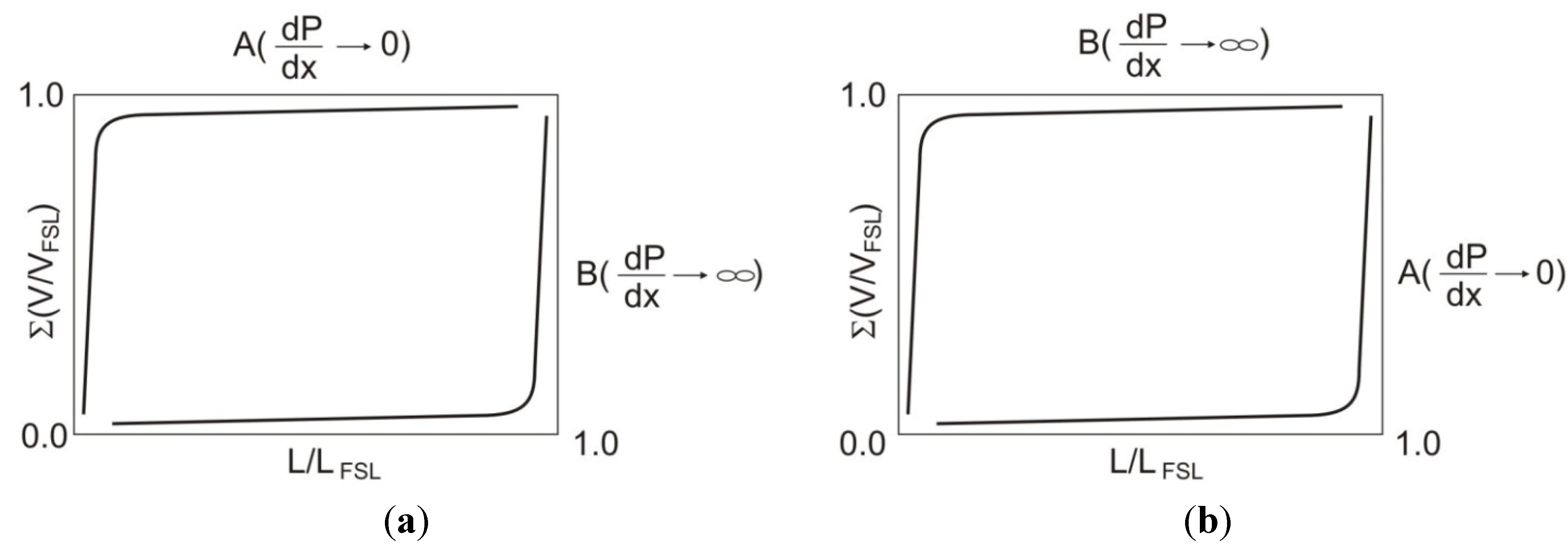
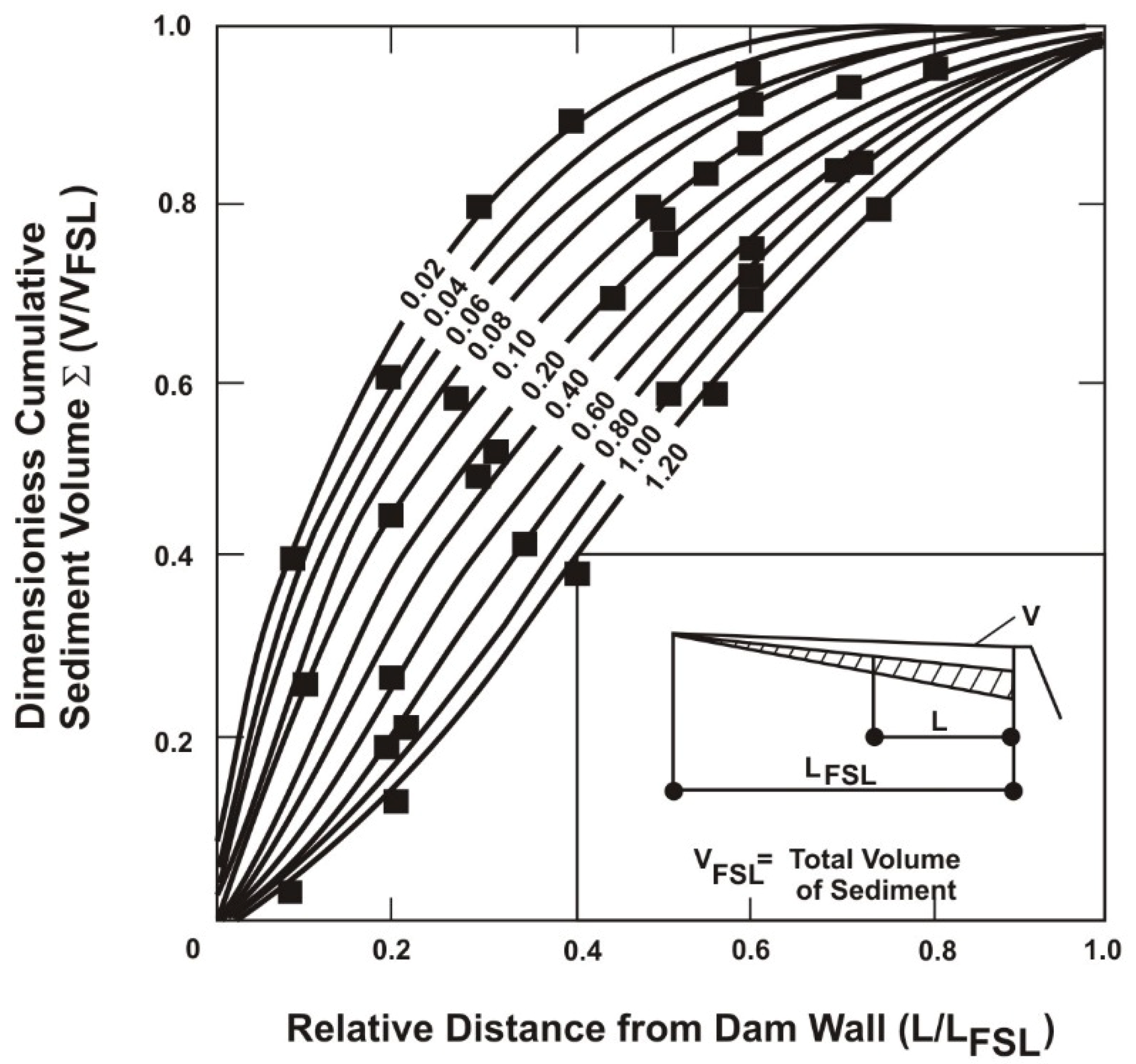
1.2. Annandale’s Method for Predicting Sediment Distribution in Reservoirs

According to the theory of stream’s energy and disposing the volumes of accumulated sediment as survey results for eleven reservoirs in South Africa, a graph relating the dimensioned cumulative volume of deposited sediment Ʃ(V/V_FSL) to the relative distance in the reservoir (L/L_FSL), for various values (dP/dx), has been compiled. In the relation (dP/dx), P is the wetted perimeter and x is the distance from the dam. This relation can be described as:

$${\displaystyle \sum \frac{\text{V}}{{\text{V}}_{\text{FSL}}}}=\text{f}\left(\frac{\text{L}}{{\text{L}}_{\text{FSL}}}\text{,}\frac{\text{dP}}{\text{dx}}\right)$$

(1)

where, V: the volume of deposited sediment; V_FSL: the total volume of sediment (at full supply level—FSL); L: the distance from the dam’s wall (it is equal to x, when L is the distance between the cross-section and the dam’s wall and for this distance the value dP/dx was elaborated); L_FSL: the total length of a reservoir (at full supply level—FSL).

The scope of Annandale’s method (Figure 1) is limited to such conditions of silting when the sediment load is deposited in the reservoir below the water table, without the formation of islands. Each line in Figure 1 represents data from same reservoir from Annandale’s field survey.

Annandale’s method [31] is one of the easiest to apply. It has been developed based on measurements of sediment load distribution in reservoirs with the capacity from 2.19 × 10⁶ m³ to 6.09·× 10⁹ m³. Even though Annandale did not survey small reservoirs, he also did not impose restrictions on size and type of reservoirs. Also the theory of stream’s energy applied in Annadale’s method is universal: a profile of deposited sediment approaches a stable condition when stream power approaches a constant minimum value throughout a reservoir. Therefore, testing this method against a small reservoir was a valid subject for this study.

This paper attempts to apply this method to determine the distribution of sediments in small reservoirs with a capacity within the range 34.5 × 10³–1100 × 10³ m³. The results of calculations using this method were compared with the results of measurements of the volume of sediment load deposits in the examined reservoirs. The results of field studies were the basis for the modification of the method. The modified Annandale’s method will allow the estimation of sediment load distribution in small reservoirs. Furthermore, a new definition of the term “small reservoir” was proposed based on the measurement results.

Figure 1. Sediment distribution within a water reservoir according to Annandale [31]. The values from 0.02 to 1.20 on solid lines represent longitudinal gradient dP/dx.

Figure 1. Sediment distribution within a water reservoir according to Annandale [31]. The values from 0.02 to 1.20 on solid lines represent longitudinal gradient dP/dx.

2. Materials and Methods

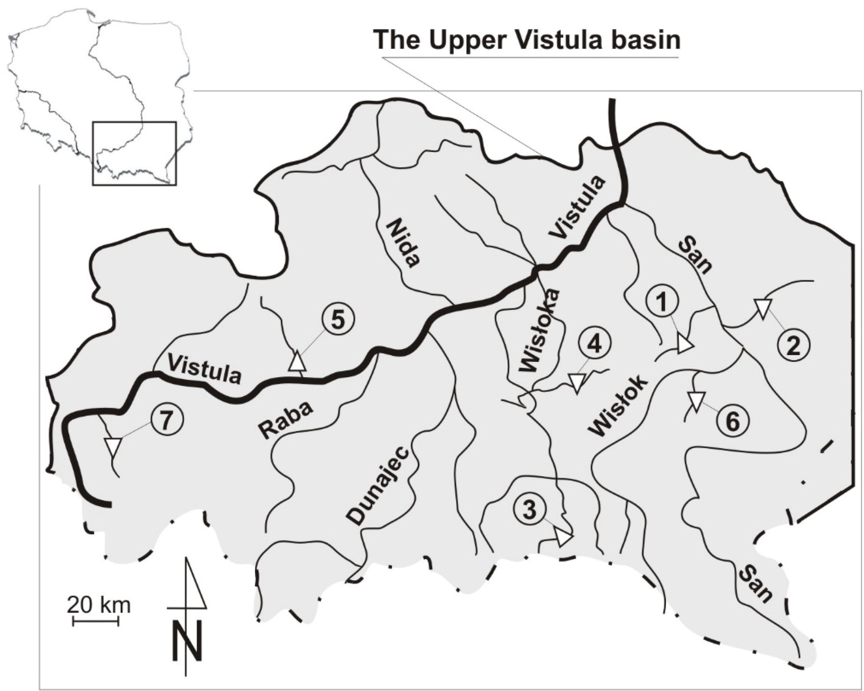
2.1. Characteristics of Research Objects

The study was conducted on eight small reservoirs, located in southern Poland (Figure 2) [39]. The basic parameters of the reservoirs are provided in Table 2.

Figure 2. Location of the examined small reservoirs.

Figure 2. Location of the examined small reservoirs.

Table 2. The selected basic parameters of the studied small water reservoirs.

Reservoir	Reservoir’s Capacity (103 m3)	Normal Water Level (m a.s.l.)	Surface of the Water Table (ha)	Mean Depth (m)	Length of the Reservoir (m)	Catchment Area (km2)
Brzóza Królewska	48.8	195.00	6.13	0.80	440	30.40
Ożanna	252.0	172.90	18.00	1.40	950	136.30
Krempna-1	119.1	370.00	3.20	3.72	400	165.30
Krempna-2	112.0	370.00	3.20	3.50	400	165.30
Cierpisz	34.5	198.90	3.20	1.50	340	54.50
Zesławice	228.0	215.00	9.50	2.40	650	218.00
Głuchów	22.6	193.60	1.50	1.51	640	12.30
Wapienica	1100.0	477.60	17.50	6.29	1000	55.50

Table 2. The selected basic parameters of the studied small water reservoirs.

Reservoir	Reservoir’s Capacity (103 m3)	Normal Water Level (m a.s.l.)	Surface of the Water Table (ha)	Mean Depth (m)	Length of the Reservoir (m)	Catchment Area (km2)
Brzóza Królewska	48.8	195.00	6.13	0.80	440	30.40
Ożanna	252.0	172.90	18.00	1.40	950	136.30
Krempna-1	119.1	370.00	3.20	3.72	400	165.30
Krempna-2	112.0	370.00	3.20	3.50	400	165.30
Cierpisz	34.5	198.90	3.20	1.50	340	54.50
Zesławice	228.0	215.00	9.50	2.40	650	218.00
Głuchów	22.6	193.60	1.50	1.51	640	12.30
Wapienica	1100.0	477.60	17.50	6.29	1000	55.50

With the exception of the reservoir Wapienica, the height of dams of the studied reservoirs is below 5 m [40]. The dam of this reservoir is 30 m high. The reservoir Krempna-2 is the same object as the reservoir Krempna-1, but its capacity was reduced by dredging and reconstruction of the inlet to the reservoir. Also reservoir Cierpisz was dredged in 1990. The first period of its operation was from 1956 to 1990, and the second period has been from 1990 to present. The main function of the studied reservoirs is to collect water for irrigation, water supply and recreation. Water outflow is controlled daily only in the Zesławice reservoir. The remaining reservoirs are the ones without daily outflow controlling.

2.2. Research Methodology

Measurements of sediment deposition volumes in the analyzed reservoirs were based on determining the changes in ordinates of the reservoir beds in cross-sections and at points outside the cross-sections. The measurements were performed with a rod probe from a boat. The measurement accuracy of bottom elevation was ±3 cm and corresponded to the thickness of the foot of the rod probe, which prevented the probe from sinking into the layer of sediment. According to Rausch and Heinemann [41], the measurements of changes in bottom height should be made with an accuracy of ±3 cm. According to these authors, the measurement error estimated with this accuracy, in the case of reservoirs with water depth of 2 m and sediment thickness of 1 m, averaged ±1.5% of the reservoir volume and ±3.0% of the sediment volume. Because of the large depth of the Wapienica reservoir, the depth measurements were performed using a Humming Bird 1000 sonar, whose detector was transformed to generate acoustic beam, with deviation from the vertical less than 3°.

The measurements of the load’s volume in the examined reservoirs were conducted within the research projects [39,42], excluding the reservoirs Krempna-1 and Zesławice. The measurements of these two water reservoirs were conducted by the University of Agriculture in Cracow in the 1970s and 1980s. The results of surveying measurements were plotted on the site and height guidelines of the reservoirs, developed during the construction of the reservoirs. The ordinates of the reservoirs’ bottom, determined based on the measurements, were plotted on these guidelines in the cross-sections of the reservoirs. Then, the areas of sediment deposits in each cross-section were determined and, knowing the distances between the cross-sections, the partial volumes of sediments and total sediment volumes in the reservoir were specified.

Subsequently, the silting ratio (S_R) and the mean annual silting ratio (S_{R, M}) were calculated. Due to the fact that the measurements of silting of the examined reservoirs were performed at different periods of operation, the silting ratio (S_R) was calculated as the ratio of the volume of sediment load deposits collected in the given operation period and the total volume of the reservoir [39]. The silting ratio enabled the identification and comparison of the capacity reduction of the reservoirs, as the comparison of the length of operation period is unreliable due to different rate of silting. The mean annual silting ratio (S_{R, M}) was calculated as the quotient of silting ratio (S_R) established over several years of operation.

The following stage of the study was to elaborate the sediment distribution in the investigated reservoirs. The partial volumes of sediments enabled the determination of partial volumes of sediment (V_FSL) deposited in sections of the reservoir from the dam to the cross-section (L), which were presented graphically and compared with the results of the forecasted sediment distribution according to the method of Annandale [31]. The application of this method requires:

(1)

the determination of the total volume of sediments in the reservoir (Ʃ V_FSL);

(2)

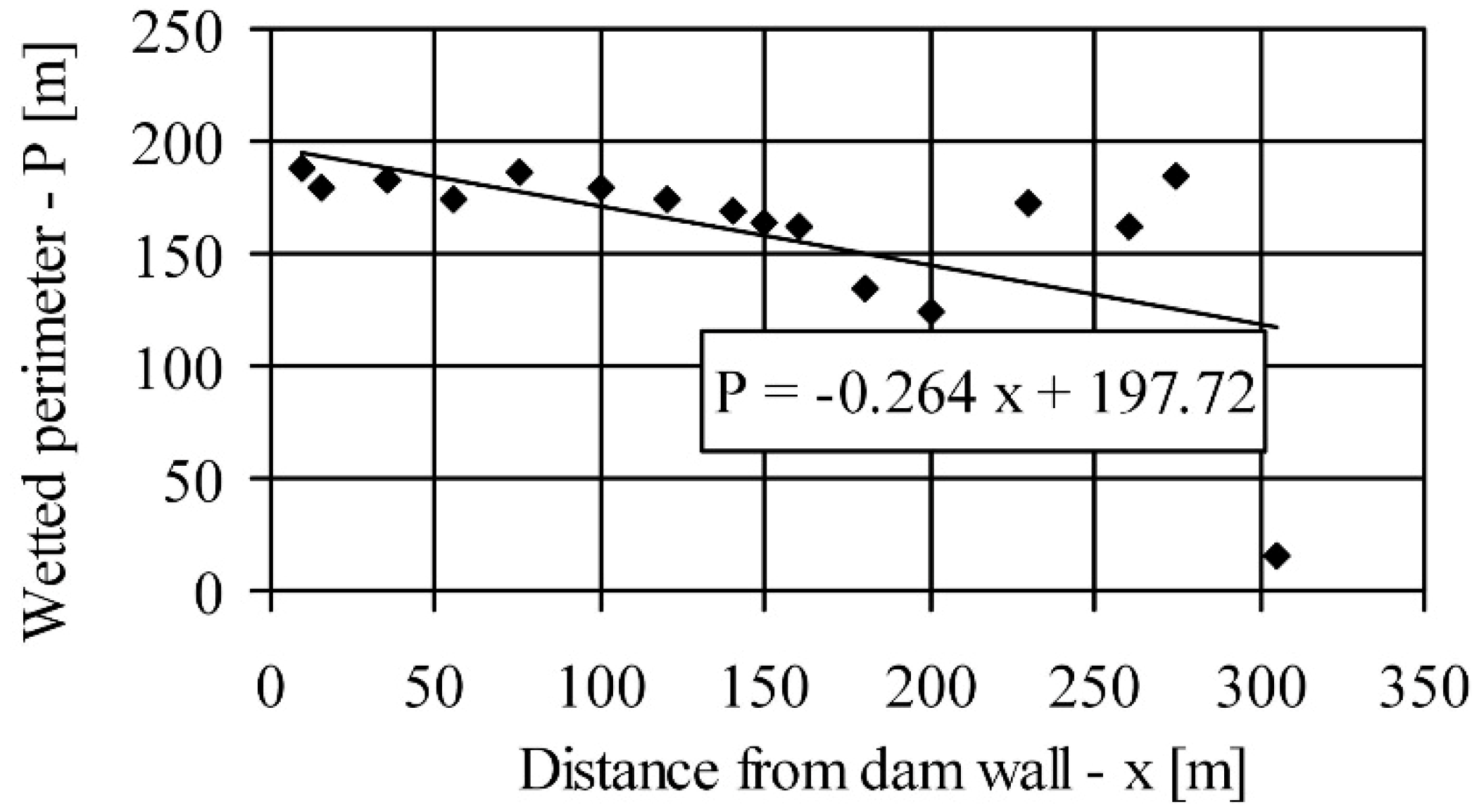
the development of mean value of longitudinal gradient dP/dx. For this purpose, a regression curve is drawn for a specific wetted perimeter (P) in each cross-section at a distance x from the dam’s wall;

(3)

the determination of the dimensioned cumulative volume of deposited sediment (Ʃ(V/V_FSL)) for each relative distance in the reservoir (L/L_FSL) from the corresponding curve dP/dx (Figure 1);

(4)

the calculation and drawing of the graph of sediment load distribution depending on the relative distance in the reservoir.

The essential characteristic of the reservoirs, i.e., the capacity-inflow ratio (C-I), was also identified as a relation of the initial volume of the reservoirs and mean annual runoff [43]. It was therefore necessary to determine the characteristic flows. Small reservoirs are usually located on streams not included in the hydrological observation networks. That is the case of the examined reservoirs, with the exception of two—Krempna and Zesławice. Due to the lack of hydrological data, characteristic flows for the cross-sections of the reservoirs were calculated using a Punzet’s [44] empirical formula for Carpathian catchments.

The Annadale’s method applicability was verified by sediment volume measurement in small water reservoirs. Also distribution of sediment over reservoir operation time was observed, i.e., whether sediment distribution curves remain constant over time. Based on Dendy’s [45] method, sediment distribution curves have been elaborated. They depict a relationship between the dimensionless cumulative volume of deposited sediment (Ʃ(V/V_FSL)) and the relative distance in the reservoir (L/L_FSL).

The last stage of the study was to determine the sediment distribution within small reservoirs. The sediment distribution curves designed based on the results of silting measurements of eight examined reservoirs were presented on a graph showing the relationship between the dimensioned cumulative volume of deposited sediment (V/V_FSL) and the relative distance in the reservoir (L/L_FSL), for different values (dP/dx).

3. Results and Discussion

3.1. Siltation Rate

The slow silting rate of Wapienica reservoir (Table 3) is due to the small sediment yield load flowing into the reservoir. Of this reservoir’s catchment, 97% is covered by forests. Due to the small size of the catchment and low intensity of erosion processes, the degree of silting is only 4.3% after over 70 years of operation. The reservoirs Głuchów and Brzóza Królewska, as well as Cierpisz, also close small-area catchments (Table 2) located in areas with reduced slopes. Such a location for the reservoirs means that the intensity of the sediment load transport to the reservoirs is small and the silting ratio after several years of operation is about 20%. The reservoirs Krempna and Zesławice are the most intensively silted. The reservoir Krempna is located in a mountainous area with intensive surface erosion, and the catchment of the reservoir Zesławice, whereby 78% of the area is used for agricultural purposes, is covered with loess. It can be observed that a small reservoir becomes silted up faster if the siltation rate reaches 20% over a dozen years of operation (Table 3), in contrast to large reservoirs that achieve that level over centuries [46,47,48,49]. Krempna-1, Krempna-2, Zesławice, Głuchów reservoirs are characterized with such fast silting up, as well as Cierpisz reservoir in the period after its desilting and rebuilding i.e., from 1990 to present (Table 3). The siltation rate of reservoirs is compared best with mean annual silting ratio—S_{R, M} (Table 3). According to Hartung [50], mean annual loss of capacity in large reservoirs is 0.25%; in medium-sized reservoirs it is above 0.5%; and in small water bodies, it is 3.0%. The S_{R, M} of Wapienica equal to 0.1% indicates that capacity reduction is typical for large reservoirs. Conversely, the siltation rate of Ożanna reservoirs is similar to medium-sized reservoirs (S_{R, M} = 0.5%).

The examined small reservoirs of the Upper Vistula basin are characterized by an intense silting rate. The silting degree after fifteen to twenty years of operation usually reaches 40%–50%. Among them, two reservoirs (Cierpisz and Wapiennica) are the exception. Small reservoirs in different climate areas around the world also silt up quickly. Dendy [51], based on research conducted in the United States on 17 small reservoirs with capacities from 22 thousand m³ to 1.17 million m³, demonstrated that after six to ten years of operation, the degree of silting ranged from less than 4% to 17%. However, after 14 years of operation, the silting degree reached 37%–65%. Much more diverse silting intensity is characteristic of small reservoirs in Tunisia. The data presented in the paper by Jebari et al. [47] indicate that some of the reservoirs after ten years of operation are silted up 30%–40%, but among them there are some reservoirs whose silting degree is only a few percent. Among 23 reservoirs analyzed in the studies of Jebari et al. [47], two of them were silted in ca. 70%, respectively, after 6 and 8 years of operation.

The examined reservoirs in the Upper Vistula basin are located in catchments, where mean annual runoff is very low (Table 3), and the determined capacity-inflow ratios are less than 1%. One exception is the reservoir Wapienica. The sediment trap efficiency of those reservoirs, determined from the Brune nomogram, is on average 12.0%–37%, while for the Głuchów reservoir it is only 2.3%, and for the reservoir Wapienica—67.7%. This would mean that the reservoirs retain only a small portion of the incoming sediment. The STE value—the sediment trap efficiency defined as the percentage of total inflowing sediment retained in a reservoir and determined from the Brune nomogram [43]—is underestimated because, as shown by the research results [40], the STE value of those reservoirs is ca. 90%.The STE of small reservoirs was determined by Michalec [40] as quotient of sediment mass deposited in the first year of operation and total sediment mass flowing into the reservoir in the first year of operation. The mass of deposited sediment was calculated from the transformed Goncharov [52] equation based on silting measurements.

Table 3. Volume of deposited sediment and silting ratio of the studied reservoirs in several years of operation [40].

Reservoir	Year	Years of Operation	Volume of Sediment V (m3)	Silting Ratio in Several Years of Operation SR (%)	Mean Annual Silting Ratio SR, M (%)
Krempna-1	1986	15	35,660	29.9	2.0
Krempna-2	1996	9	27,040	24.1	2.7
	1997	10	30,460	27.2	2.7
	1998	11	34,640	30.9	2.8
	1999	12	38,000	33.9	2.8
	2000	13	40,140	35.8	2.8
	2002	15	44,200	39.5	2.6
	2003	16	44,900	40.1	2.5
	2005	18	45,810	40.9	2.3
Zesławice	1968	2	26,970	11.8	5.9
	1969	3	70,430	30.9	10.3
	1970	4	75,780	33.2	8.3
	1971	5	76,250	33.4	6.7
	1974	8	86,190	37.8	4.7
	1983	17	116,090	50.9	3.0
Głuchów	2002	7	4,130	18.3	2.6
	2009	14	5,890	26.1	1.9
Brzóza Królewska	2002	7	4,180	8.5	1.2
	2009	14	6,400	13.1	0.9
Ożanna	1998	20	26,000	10.3	0.5
	2003	25	30,200	12.0	0.5
Cierpisz	1990	34	15,000	43.5	1.3
	2001	11	6,100	17.7	1.6
	2003	13	6,750	19.6	1.5
Wapienica	1967	36	24,250	2.2	0.1
	2003	71	46,800	4.3	0.1

Table 3. Volume of deposited sediment and silting ratio of the studied reservoirs in several years of operation [40].

Reservoir	Year	Years of Operation	Volume of Sediment V (m3)	Silting Ratio in Several Years of Operation SR (%)	Mean Annual Silting Ratio SR, M (%)
Krempna-1	1986	15	35,660	29.9	2.0
Krempna-2	1996	9	27,040	24.1	2.7
	1997	10	30,460	27.2	2.7
	1998	11	34,640	30.9	2.8
	1999	12	38,000	33.9	2.8
	2000	13	40,140	35.8	2.8
	2002	15	44,200	39.5	2.6
	2003	16	44,900	40.1	2.5
	2005	18	45,810	40.9	2.3
Zesławice	1968	2	26,970	11.8	5.9
	1969	3	70,430	30.9	10.3
	1970	4	75,780	33.2	8.3
	1971	5	76,250	33.4	6.7
	1974	8	86,190	37.8	4.7
	1983	17	116,090	50.9	3.0
Głuchów	2002	7	4,130	18.3	2.6
	2009	14	5,890	26.1	1.9
Brzóza Królewska	2002	7	4,180	8.5	1.2
	2009	14	6,400	13.1	0.9
Ożanna	1998	20	26,000	10.3	0.5
	2003	25	30,200	12.0	0.5
Cierpisz	1990	34	15,000	43.5	1.3
	2001	11	6,100	17.7	1.6
	2003	13	6,750	19.6	1.5
Wapienica	1967	36	24,250	2.2	0.1
	2003	71	46,800	4.3	0.1

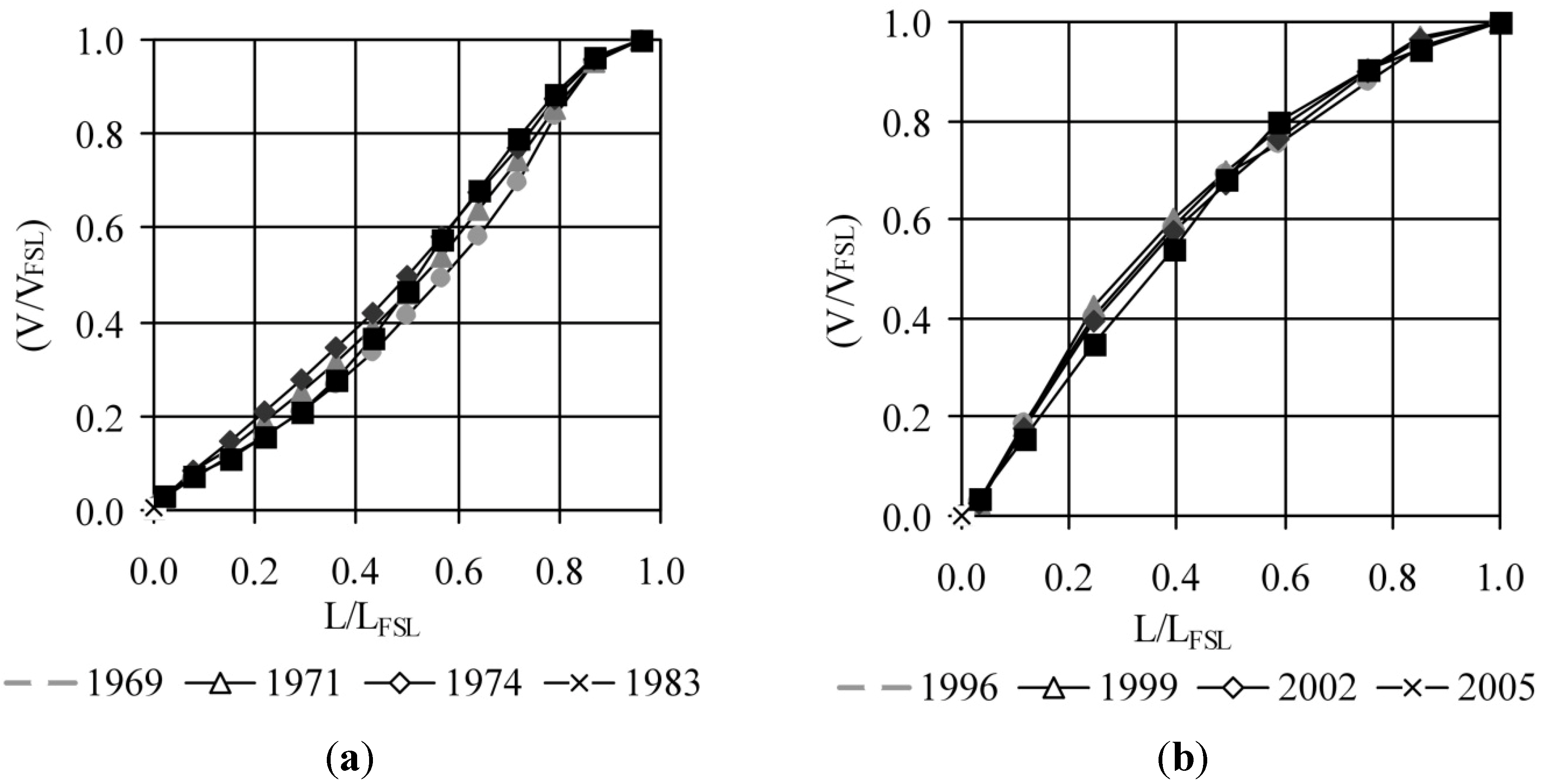
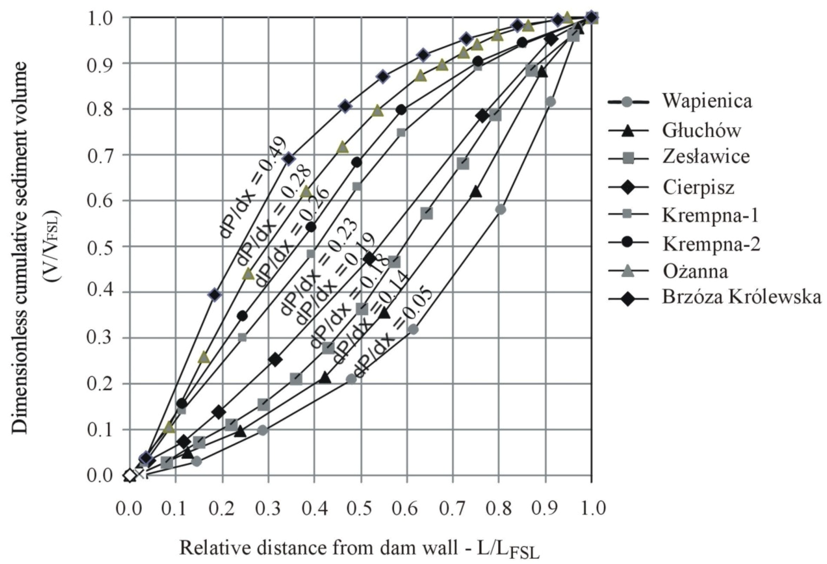
3.2. Sediment Distribution

When trying to apply Annandale’s method [31] to determine the sediment load distribution in small reservoirs, segments were separated in each of the reservoirs. These segments constituted partial volumes contained between adjacent cross-sections. The volume of accumulated sediment load, determined based on field measurements, was identified in these segments. Subsequently, regression relationships were identified for specific wetted perimeters (P) and distances from the dam’s wall (x) of each cross-section of the reservoir. The exemplary relationship identified for the reservoir Krempna-2 is shown in Figure 3.

Figure 3. Relationship between the wetted perimeter (P) and the distance from the dam (x) established for the water reservoir Krempna-2.

Figure 3. Relationship between the wetted perimeter (P) and the distance from the dam (x) established for the water reservoir Krempna-2.

At this point, attention should be paid to the method of determining the longitudinal gradient dP/dx, which in the above example is 0.264, determined for the distance x given in meters. Annandale calculated the values of longitudinal gradients (Figure 1) for distances x in kilometers. The examined small reservoirs are from 440 to 1000 m long. The length of the reservoirs studied by Annadale [31] ranged from several to a few dozen kilometers. When adopting the distance x for the exemplary reservoir Krempna-2 in kilometers, the obtained longitudinal gradient dP/dx would be 264.0, i.e., a value beyond the scope given in Figure 1, in which the sediment distribution curve values dP/dx range from 0.02 to 1.20. The values dP/dx determined according to the methodology of Annandale [31] are a thousand times larger than the ones given in Table 4. It appears that the use of the sediment distribution curves (Figure 1) is impossible. The values dP/dx calculated with the distance in meters, but not in kilometers, will enable the comparison of sediment distribution according to the function given in Figure 1 and determined based on field measurements.

Table 4. Longitudinal gradient (dP/dx) and capacity-inflow ratio (C-I) in the studied reservoirs.

Reservoir	Longitudinal Gradient dP/dx (-)	Mean Annual Runoff Q (m3·s−1)	Capacity-Inflow Ratio C-I (%)
Brzóza Królewska	0.49	0.224	0.69
Ożanna	0.28	1.006	0.79
Krempna-1	0.23	2.030	0.37
Krempna-2	0.26	2.030	0.35
Cierpisz	0.19	0.393	0.28
Zesławice	0.18	0.709	0.66
Głuchów	0.14	0.567	0.13
Wapienica	0.05	0.120	2.91

Table 4. Longitudinal gradient (dP/dx) and capacity-inflow ratio (C-I) in the studied reservoirs.

Reservoir	Longitudinal Gradient dP/dx (-)	Mean Annual Runoff Q (m3·s−1)	Capacity-Inflow Ratio C-I (%)
Brzóza Królewska	0.49	0.224	0.69
Ożanna	0.28	1.006	0.79
Krempna-1	0.23	2.030	0.37
Krempna-2	0.26	2.030	0.35
Cierpisz	0.19	0.393	0.28
Zesławice	0.18	0.709	0.66
Głuchów	0.14	0.567	0.13
Wapienica	0.05	0.120	2.91

By applying Annandale’s method [31], the longitudinal gradient dP/dx was determined for distances x given in meters. The values dP/dx calculated for Krempna-1 and Krempna-2 reservoirs are 0.23 and 0.26, respectively. Due to geometry unaltered by dredging and reconstruction, the value dP/dx for the reservoirs Zesławice-1 and Zesławice-2 equals 0.18. The dP/dx values for the remaining reservoirs are given in Table 4, where the calculated mean annual runoff (Q) and capacity-inflow ratio (C-I) are also presented.

Capacity-inflow ratio of the examined reservoirs is less than 1%, except for Wapienica reservoir for which C-I is equal to 2.91 (Table 4). However, mean annual silting ratio (S_{R, M}) of these reservoirs (Table 3) is from 0.5% to 10.3%. Such silting ratios according to Hartung [50] correspond to siltation rate of small reservoirs. Therefore, a small reservoir in the Upper Vistula basing can be defined as such that has the capacity-inflow ratio below 1%.

The forecast of sediment load distribution was prepared for eight examined reservoirs. In the case of the reservoirs Krempna-1 and Krempna-2, the course of sediment load distribution curve, defined by the calculations, is similar to the curve determined based on the measurements (Table 5, Figure 4). The sediment load accumulates in the near-dam zone of the Krempna reservoir, thus in accordance with the assumptions of Annandale’s method. Silting of the reservoir Brzóza Królewska proceeds in a similar way. Segments of the near-dam and central zones of these reservoirs are characterized by the highest relative silting, expressed by the silting ratio of each segment.

Table 5. Comparison of the results of sediment distribution forecast in the reservoir Krempna-2 according to Annandale’s method [31] (A. method) and results of silting measurements (measure.) in 1996.

Segment	L/LFSL	Σ(V/VFSL)	V/VFSL	Volume of Deposited Sediment (m3)
				A. Method	Measure.
1	0.03	0.05	0.05	1,351	877
2	0.11	0.21	0.16	4,327	4,150
3	0.25	0.43	0.22	5,949	5,900
4	0.39	0.62	0.19	5,138	4,959
5	0.49	0.72	0.10	2,704	2,763
6	0.59	0.81	0.09	2,434	1,657
7	0.75	0.90	0.09	2,433	3,401
8	0.85	0.95	0.05	1,352	1,931
9	1.00	1.00	0.05	1,352	1,402
Sum			1.00	27,040	27,040

Table 5. Comparison of the results of sediment distribution forecast in the reservoir Krempna-2 according to Annandale’s method [31] (A. method) and results of silting measurements (measure.) in 1996.

Segment	L/LFSL	Σ(V/VFSL)	V/VFSL	Volume of Deposited Sediment (m3)
				A. Method	Measure.
1	0.03	0.05	0.05	1,351	877
2	0.11	0.21	0.16	4,327	4,150
3	0.25	0.43	0.22	5,949	5,900
4	0.39	0.62	0.19	5,138	4,959
5	0.49	0.72	0.10	2,704	2,763
6	0.59	0.81	0.09	2,434	1,657
7	0.75	0.90	0.09	2,433	3,401
8	0.85	0.95	0.05	1,352	1,931
9	1.00	1.00	0.05	1,352	1,402
Sum			1.00	27,040	27,040

Figure 4. Sediment distribution in the reservoir Krempna-2 in 2000 determined according to measurements and Annandale’s method.

Figure 4. Sediment distribution in the reservoir Krempna-2 in 2000 determined according to measurements and Annandale’s method.

The calculated amount of the deposited sediment load according to Annandale’s method is greater than the one measured in the segments closest to the dam. The further from the dam, the smaller the difference between the results becomes, amounting only to a few percent. The exemplary graph of sediment load distribution in 2000, calculated using Annandale’s method [31] and determined according to the measurements, are presented in Figure 4.

The sediment is deposited at the inlet rather than near the dam wall. Only in the case of two reservoirs, Krempna-2 and Brzóza Królewska, is the sediment deposited near the dam, just as predicted by the Annandale’s calculations. All other reservoirs used in this research have higher amounts of deposits located closer to their inlets. For this reason, the results of sediment distribution forecast in small reservoirs according to Annandale’s method [31] do not correspond to the actual state. The examples are given below calculations of sediment load deposits in the reservoir Zesławice-1 in 1974 (Table 6) and 1983 (Figure 5). Segments at the inlet to the reservoir are characterized by the greatest relative silting, while according to calculations using Annandale’s method [31], their relative silting will be significantly smaller.

Table 6. Comparison of the results of sediment distribution forecast in the reservoir Zesławice according to Annandale’s method [31] (A. method) and results of silting measurements (measure.) in 1974.

Segment	L/LFSL	Σ(V/VFSL)	V/VFSL	Volume of Deposited Sediment (m3)
				A. Method	Measure.
1	0.02	0.03	0.03	2585	84
2	0.08	0.18	0.15	12,929	2,119
3	0.15	0.30	0.12	10,343	5,137
4	0.22	0.42	0.12	10,343	5,275
5	0.29	0.53	0.11	9,481	5,467
6	0.36	0.62	0.09	7,757	5,865
7	0.43	0.70	0.08	6,895	5,920
8	0.50	0.76	0.06	5,172	6,060
9	0.57	0.82	0.06	5,172	6,852
10	0.64	0.87	0.05	4,310	7,512
11	0.72	0.90	0.03	2,585	7,889
Sum			1.00	86,190	86,190

Table 6. Comparison of the results of sediment distribution forecast in the reservoir Zesławice according to Annandale’s method [31] (A. method) and results of silting measurements (measure.) in 1974.

Segment	L/LFSL	Σ(V/VFSL)	V/VFSL	Volume of Deposited Sediment (m3)
				A. Method	Measure.
1	0.02	0.03	0.03	2585	84
2	0.08	0.18	0.15	12,929	2,119
3	0.15	0.30	0.12	10,343	5,137
4	0.22	0.42	0.12	10,343	5,275
5	0.29	0.53	0.11	9,481	5,467
6	0.36	0.62	0.09	7,757	5,865
7	0.43	0.70	0.08	6,895	5,920
8	0.50	0.76	0.06	5,172	6,060
9	0.57	0.82	0.06	5,172	6,852
10	0.64	0.87	0.05	4,310	7,512
11	0.72	0.90	0.03	2,585	7,889
Sum			1.00	86,190	86,190

Figure 5. Sediment distribution in the reservoir Zesławice-1 in 1983 determined according to measurements and Annandale’s method [31].

Figure 5. Sediment distribution in the reservoir Zesławice-1 in 1983 determined according to measurements and Annandale’s method [31].

Annandale [31] developed the relationship presented in Figure 1 for 11 reservoirs, whose silting degree ranged between 7.85% and 44.94%. This relationship was developed for the results of silting measurements of reservoirs with various silting ratios (S_R). Annandale did not consider the variability of sediment distribution in the reservoir depending on its silting ratio. Figure 6a,b present the relative sediment load distribution in the reservoirs Krempna-2 and Zesławice, respectively. The sediment distribution curves change slightly with the increase in the silting ratio, which was observed in all examined reservoirs. In the reservoir, where the sediments are retained mainly in the middle and the inlet zone, these zones of the reservoir are characterized by increased relative volume of sediment load deposits. One example is the reservoir in Zesławice (Figure 5a)—in the part of the reservoir from 0.35 to 0.8 of the relative distance from the dam there was a significant increase in sediment load deposits in 1983 (S_R = 50.9%), as compared to 1969 (S_R = 30.9%). In the reservoir Krempna-12, where the sediment load is accumulated according to the course of distribution curves presented by Annandale (Figure 1), i.e., its greatest volume is deposited in the near-dam zone of the reservoir, the relative volume of sediments accumulated in the near-dam and central zone decreased together with the increase of silting ratio. Within nine years there was a small reduction in relative volume of sediments in the section from 0.11 to 0.5 of the relative distance from the dam of the reservoir Krempna-2 (Figure 6b) with the increase of silting degree from 24.2% to 40.9%. After analyzing these examples, it may be stated that the change in silting degree, even by about 20%, has a negligible impact on the sediment distribution curves in the reservoirs.

Figure 6. Sediment distribution within water reservoirs: (a) Zesławice and (b) Krempna-2 in several years of operation.

Figure 6. Sediment distribution within water reservoirs: (a) Zesławice and (b) Krempna-2 in several years of operation.

Dendy [51] in his paper did not present the results of measurements of deposit volumes in different parts of the reservoirs. He only stated that “most of the sediment was deposited in the upstream end of the reservoirs near the elevation of the conservation pool. Proportion of the total sediment deposited in the sediment pool ranged from 30 to 100 percent.” Dendy [45] presented the distribution of sediments on the graph of horizontal distribution of sediment deposits indicating that the sediment in these reservoirs is deposited mainly at the inlet to the reservoir, or at most proportionally to the ratio of the conservation pool volume upstream from a given location (V) to the total volume (V_t) of the conservation pool, designated as V/V_t. For two reservoirs, the horizontal distribution of sediment deposits developed by Dendy shows a proportional increase in the volume of sediment deposits to the increase in the value of V/V_t. This means that in some reservoirs, a significant portion of the sediment is deposited closer to the dam. Unfortunately, Dendy [45] in his paper did not present the geometric characteristics of the reservoirs, which would allow verification of the proposed modification of the Annandale’s method.

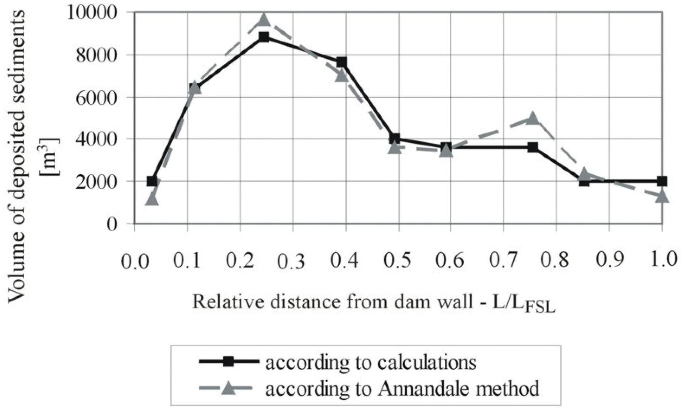
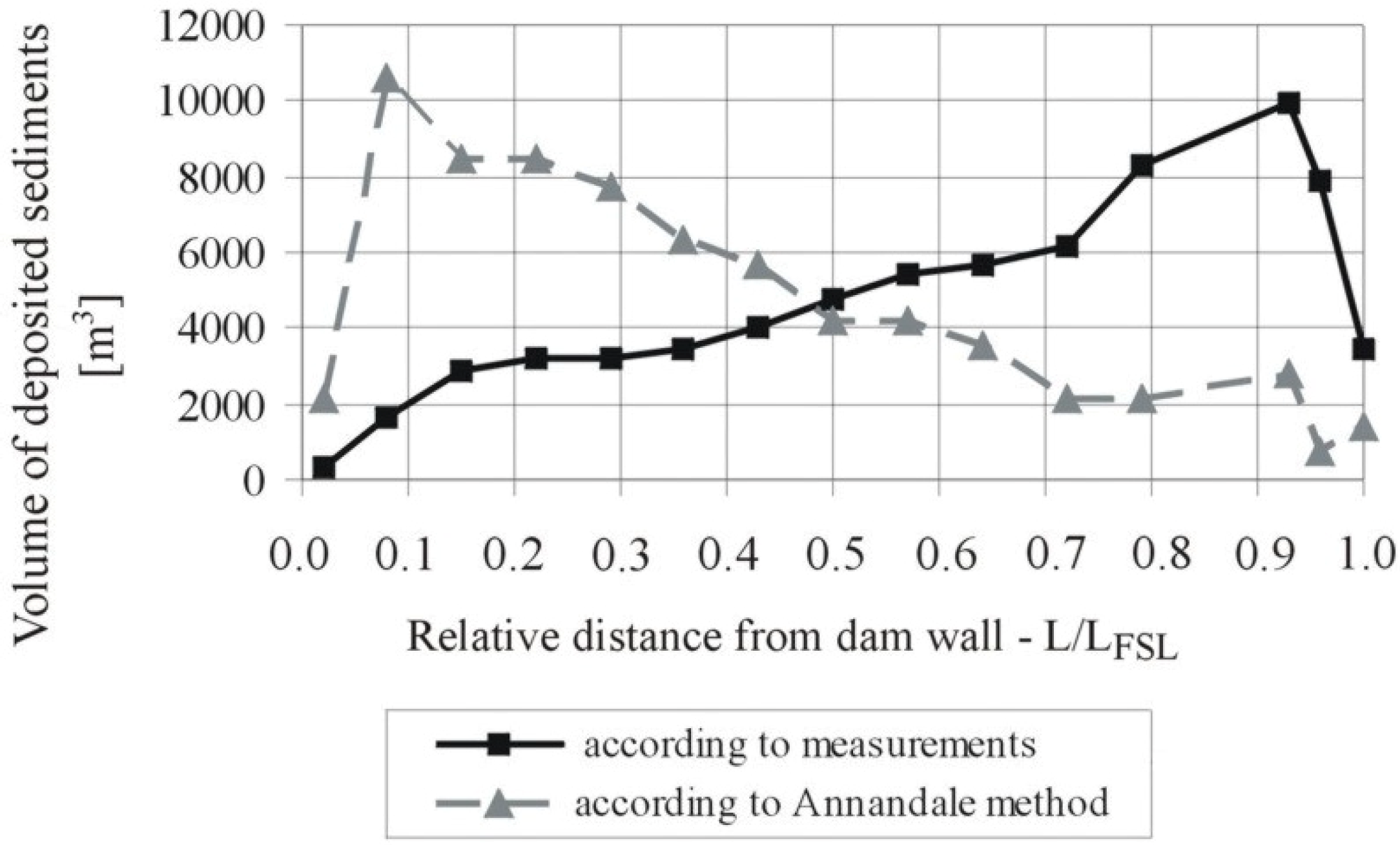
3.3. Modification of the Annandale Method

A graph presenting the dependence between the sum of dimensionless sediment load volume Σ(V/V_FSL) as a function of relative distance from the dam L/L_FSL (Figure 7) was developed based on the results of silting measurements of the examined small reservoirs.

Figure 7. Sediment distribution within small reservoirs. The points were established according to a field survey for separated segments of examined reservoirs.

Figure 7. Sediment distribution within small reservoirs. The points were established according to a field survey for separated segments of examined reservoirs.

According to Annandale [31], the relationship between the dimensionless cumulative mass curves explaining sediment distribution as a function of dP/dx (Figure 1) was verified through the identified limits. If dP/dx → 0, it corresponds with the situation where only a small disturbance exists in the channel. As Annandale reported [31], under such circumstances the sediment will be deposited in the proximity of the disturbance with very little build-up in the upstream direction. The dimensionless cumulative curve will then have a shape as shown by curve A in Figure 8a. As demonstrated by the analysis of the curves dP/dx on the graph developed by Annandale (Figure 1), in such conditions the sediment is deposited by the dam. For dP/dx of 0.02 over 60% of sediment is deposited in the relative distance of 0.2 from the dam. On the other hand, when dP/dx → ∞, a condition similar to a river flowing into an ocean exists, and the major volume of sediment will be deposited in the vicinity of the river mouth (curve B in Figure 8a). This is illustrated by the curve dP/dx with the value of 1.20 (Figure 1)—the sediment will be relatively proportionally distributed over the entire length of the reservoir.

It means that in 11 reservoirs studied by Annadale, sediment is transported through the whole reservoir and deposited in segments near the dam wall. The higher the longitudinal gradient of the reservoir, the more even sediment distribution is over the reservoir segments. The study of the Upper Vistula reservoirs indicates that sediment is deposited evenly over the whole length of the reservoirs when longitudinal gradient reaches the value of ca. 0.19 (see Cierpisz reservoir—Figure 7). In small reservoirs of Upper Vistula, this situation is inverted compared to Annadale’s: the higher the longitudinal gradient, the more the sediment is deposited near the dam wall. The results obtained from the studies of small reservoirs located in the Upper Vistula basin indicate a different arrangement of curves dP/dx (Figure 7) compared to the relationship given by Annandale (Figure 1). In the case of the examined reservoirs, when dP/dx → 0, it corresponds to the situation when less sediment is deposited in the near-dam zone, while the predominant portion is deposited at the inlet to the reservoir (curve A in Figure 8b). However, in conditions corresponding to the ratio dP/dx tending to infinity, the sediment is deposited near the dam wall (curve B in Figure 8b).

Figure 8. Extremes of dimensionless curves: (a) according to Annandale [31]; (b) according to the results of experiments on small reservoirs located in the Upper Vistula basin.

Figure 8. Extremes of dimensionless curves: (a) according to Annandale [31]; (b) according to the results of experiments on small reservoirs located in the Upper Vistula basin.

4. Conclusions

Annandale’s method was developed based on silting measurements of reservoirs, whose length was from a few to several dozen kilometers. The application of this method in its original form to determine the sediment deposition in small reservoirs, with a capacity less than 5 million m³, is possible only in the case of reservoirs, in which the sediments are deposited in the near-dam zone. Among the reservoirs analyzed in this research, such conditions of sediment deposition were recorded in two reservoirs—Krempna and Brzóza Królewska. Although the predicted sediment distribution differed from the results obtained from measurements, the approximate sediment distribution in these reservoirs may be determined using the original Annandale method.

Annandale’s method in its original form may not be applied to determine the sediment deposition in small reservoirs, whose:

-

length is less than 1000 m;

-

capacity-inflow ratio ranges from a few per mille to a percent.

The forecast of the sediment distribution in small reservoirs with capacities below 1.1 million m³ is possible using the sediment distribution graph, introduced in Figure 7. This is allowed by the modified Annandale method, presented in this paper and developed based on the results of silting measurements of eight small reservoirs.

Due to the lack of access to measurement results of segmented sediment volume depositions in small reservoirs from different regions of the world, the proposed method requires further modification. The presented results are a contribution to supplement and correct the proposed modification of Annandale’s method.

References

1. Mahmood, K. Reservoir Sedimentation: Impact, Extent and Mitigation; Technical Paper No. 71; The World Bank: Washington, DC, USA, 1987. [Google Scholar]
2. Hotchkiss, R.H.; Parker, G. Shock fitting of aggradational profiles due to backwater. J. Hydraul. Eng. 1991, 117, 1129–1144. [Google Scholar] [CrossRef]
3. Fan, J.; Morris, G. Reservoir sedimentation. I: Delta and density current deposits. J. Hydraul. Eng. ASCE 1992, 118, 354–369. [Google Scholar] [CrossRef]
4. Sloff, C.J. Sedimentation in Reservoirs. Ph.D. Thesis, Technical University of Delft, Delft, The Netherlands, 15 April 1997. [Google Scholar]
5. De Cesare, G.; Schleiss, A.; Hermann, F. Impact of Turbidity Currents on Reservoir Sedimentation. J. Hydraul. Eng. ASCE 2001, 127, 6–16. [Google Scholar] [CrossRef]
6. Batuca, G.D.; Jordaan, M.J., Jr. Silting and Desilting of Reservoirs; A.A. Balkema: Rotterdam, The Netherlands, 2000. [Google Scholar]
7. Dewals, B.J.; Kantoush, S.A.; Erpicum, S.; Pirotton, M.; Schleiss, A.J. Experimental and numerical analysis of flow instabilities in rectangular shallow basins. Environ. Fluid Mech. 2008, 8, 31–54. [Google Scholar] [CrossRef]
8. Dufresne, M.; Dewals, B.J.; Erpicum, S.; Archambeau, P.; Pirotton, M. Classification of flow patterns in rectangular shallow reservoirs. J. Hydraul. Res. 2010, 48, 197–204. [Google Scholar] [CrossRef]
9. Camnasio, E.; Orsi, E.; Schleiss, A. Experimental study of velocity fields in rectangular shallow reservoirs. J. Hydraul. Res. 2011, 49, 352–358. [Google Scholar] [CrossRef]
10. Lane, E. Some Hydraulic Engineering Aspects of Density Currents; Hydraulic Laboratory Report No. Hyd-373; U.S. Bureau of Reclamation: Denver, CO, USA, 1954.
11. Normark, W.R.; Dickson, F.H. Man-made turbidity currents in Lake Superior. Sedimentology 1976, 23, 815–831. [Google Scholar] [CrossRef]
12. Lambert, A. Turbidity currents from the Rhine River on the bottom of Lake Constance. Wasserwirtschaft 1982, 72, 1–4. (In German) [Google Scholar]
13. Chikita, K. A field study on turbidity currents initiated from spring runoffs. Water Resour. Res. 1989, 25, 257–271. [Google Scholar] [CrossRef]
14. Boix-Fayos, C.; de Vente, J.; Martinez-Mena, M.; Barbera, G.G.; Castillo, V. The impact of land use change and check-dams on catchment sediment yield. Hydrol. Process. 2008, 22, 4922–4935. [Google Scholar] [CrossRef]
15. Leigh, C.A.; Burford, M.A.; Connolly, R.M.; Olley, J.M.; Saeck, E.; Sheldon, F.; Smart, J.C.R.; Bunn, S.E. Science to Support Management of Receiving Waters in an Event-Driven Ecosystem: From Land to River to Sea. Water 2013, 5, 780–797. [Google Scholar] [CrossRef]
16. McBroom, M.; Thomas, T.; Zhang, Y. Soil Erosion and Surface Water Quality Impacts of Natural Gas Development in East Texas, USA. Water 2012, 4, 944–958. [Google Scholar] [CrossRef]
17. Murthy, B.N. Life of Reservoir; Technical Report No. 19; Central Board of Irrigation and Power: New Delhi, India, 1977. [Google Scholar]
18. Sloff, C.J. Reservoir Sedimentation: A Literature Survey; Communications on Hydraulic and Geotechnical Engineering, Report No. 91-2; Faculty of Civil Engineering, Delft University of Technology: Delft, The Netherlands, 1991. [Google Scholar]
19. Lara, J.M.; Pemberton, E.L. Initial weight of deposited sediments. In Proceedings of the Federal Inter-Agency Sedimentation Conference, Jackson, MS, USA, 28 January–1 February 1963; USDA-ARS, Miscellaneous Publications: Jackson, MS, USA, 1963; Volume 970, pp. 818–845. [Google Scholar]
20. Program of Small Retention of the Małopolski District; Project of Marshal Office of Małopolski District and Land Melioration and Water Units Board of Małopolski Province in Cracow: Cracow, Poland, 2004; p. 47. (In Polish)
21. White, P.; Labadz, J.C.; Buchter, D.P. Sediment yield estimation from reservoir studies: An appraisal of variability in the southern Pennines of the UK. In Erosion and Sediment Yield. Global and Regional Perspectives; International Association of Hydrological Sciences Publication: Exeter, UK, 1996; Volume 236, pp. 163–173. [Google Scholar]
22. Senzanje, A.; Chimbari, M. Inventory of Small Dams in Africa—A Case Study for Zimbabwe; Draft Report for Water, Health and Environment; The International Management Institute (IWMI): Colombo, Sri Lanka, 2002. [Google Scholar]
23. Neto, I.E.L.; Wiegand, M.C.; de Araújo, J.C. Sediment redistribution due to a dense reservoir network in a large semi-arid Brazilian basin. Hydrol. Sci. J. 2011, 56, 319–333. [Google Scholar] [CrossRef]
24. Cristofano, E.A. Area-Increment Method for Distributing Sediment in a Reservoir; US Bureau of Reclamation: Albuquerque, NM, USA, 1953.
25. Borland, W.M.; Miller, C.R. Distribution of sediment in large reservoirs. J. Hydraul. Eng. Div. ASCE 1958, 84, 1–18. [Google Scholar]
26. Lara, J.M. Revision of the Procedure to Compute Sediment Distribution in Large Reservoirs; US Bureau of Reclamation: Denver, CO, USA, 1962.
27. Hobbs, B.L. Forecasting Distribution of Sediment Deposits in Large Reservoirs; Appendix I, ETL 1110-2-64; Department of the Army, Office of the Chief of Engineers: Washington, DC, USA, 1969.
28. Borland, W.M. Reservoir Sedimentation, River Mechanics; Shen, H.W., Ed.; Water Resources Publisher: Fort Collins, CO, USA, 1970; Chapter 29; pp. 1–38. [Google Scholar]
29. Pemberton, E.L. Reservoir Sedimentation. In Proceedings of the US-Japan Seminar on Sedimentation and Erosion, Honolulu, HI, USA, 20–24 March 1978.
30. Qian, N. Reservoir sedimentation and slope stability, technical and environmental effects. General Report, G.R.54. In Proceedings of the 14th International Commission on Large Dams Congress, Rio de Janeiro, Brazil, 14–17 May 1982.
31. Annandale, G.W. Predicting the distribution of deposited sediment in southern African reservoirs. In Challenges in African Hydrology and Water Resources (Proceedings of the Harare Symposium, July 1984); International Association of Hydrological Sciences Publication: Harare, Zimbabwe, 1984; Volume 144, pp. 549–558. [Google Scholar]
32. Mohammadzadeh-Habibi, J.; Heidarpour, M. New empirical method for prediction of sediment distribution in reservoirs. J. Hydrol. Eng. 2010, 15, 813–821. [Google Scholar] [CrossRef]
33. Rahmanian, M.R.; Banhashemi, M.A. A new empirical reservoir shape function to define sediment distribution pattern in dam reservoirs. IJST Trans. Civ. Eng. 2012, 36, 79–92. [Google Scholar]
34. Michalec, B. Qualification of the distribution of bottom sediments in small water reservoir using the relative depth shape. Funct. Eng. Prot. Environ. 2013, 16, 425–434. (In Polish) [Google Scholar]
35. Rooseboom, A. Reservoir sediment deposition rates. In Proceedings of the 12th ICOLD Congress, Mexico City, Mexico, 29 March–2 April 1976; pp. 184–196.
36. Verstraeten, G.; Poesen, J. Estimating trap efficiency of small reservoirs and ponds: Methods and implications for the assessment of sediment yield. Prog. Phys. Geogr. 2000, 24, 219–251. [Google Scholar] [CrossRef]
37. Verstraeten, G.; Poesen, J. Modelling the long-term sediment trap efficiency of small ponds. Hydrol. Process. 2001, 15, 2797–2819. [Google Scholar]
38. Bussi, G.; Rodríguez-Lloveras, X.; Francés, F.; Benito, G.; Sánchez-Moya, Y.; Sopeña, A. Sediment yield model implementation based on check dam infill stratigraphy in a semiarid Mediterranean catchment. Hydrol. Earth Syst. Sci. 2013, 17, 3339–3354. [Google Scholar]
39. Tarnawski, M.; Michalec, B. Assessment of Agricultural Utilization of Bottom Sediment; Research Project No. N305 295037 (2009–2012); Ministry of Science and High Education: Kraków, Poland, 2012. (In Polish)
40. Michalec, B. Appraisal of silting intensity of small water reservoirs in the Upper Vistula river basin. In Scientific Fascicles; Agricultural University Cracow: Kraków, Poland, 2008; p. 193. (In Polish) [Google Scholar]
41. Rausch, D.L.; Heinemann, H.G. Measurement of reservoir sedimentation. In Erosion and Sediment Yield:Some Methods of Measurement and Modelling; Geobooks: Norwich, England, 1984; pp. 179–200. [Google Scholar]
42. Bednarczyk, T.; Michalec, B.; Tarnawski, M. The Evaluation of the Silting Ratio of Small Reservoirs in Carpathians and Silting Forecast on the Background of Erosion Processes in the Catchments; Research Project No. 6 P06S 016 21 (1998–2001); Ministry of Science and High Education: Kraków, Poland, 2001. (In Polish)
43. Brune, G.M. Trap efficiency of reservoirs. Trans. Am. Geophys. Union 1953, 34, 407–418. [Google Scholar] [CrossRef]
44. Punzet, J. The Resources the Water Drainage Areas of the Upper Vistula. Average Flows—Seasonal Distribution and Changeability in Time and Space; Polish Scientific Publishers PWN: Warsaw, Poland, 1983; Volume 192. (In Polish) [Google Scholar]
45. Dendy, F.E. Distribution of sediment deposits in small reservoirs. Trans. Am. Soc. Agric. Eng. 1982, 25, 100–104. [Google Scholar] [CrossRef]
46. Garg, V.; Jothiprakash, V. Trap efficiency estimation of a large reservoirs. ISJ J. Hydraul. Eng. 2008, 14, 88–101. [Google Scholar] [CrossRef]
47. Jebari, S.; Berndtsson, R.; Bahri, A.; Boufaroua, M. Spatial soil loss risk and reservoir siltation in semi-arid Tunisia. Hydrol. Sci. J. 2010, 55, 121–137. [Google Scholar] [CrossRef]
48. Heidarnejad, M.S.; Golmaee, S.H.; Mosaedi, A.; Ahmadi, M.Z. Estimation of sediment volume in Karaj Dam Reservoir (Iran) by hydrometry method and a comparison with hydrography method. Lake Res. Manag. 2006, 22, 233–239. [Google Scholar] [CrossRef]
49. Araújo, J.C.; Günter, A.; Bronstert, A. Loss of reservoir volume by sediment deposition and its impact on water availability in semiarid Brazil. Hydrol. Sci. J. 2006, 51, 157–170. [Google Scholar] [CrossRef]
50. Hartung, F. Ursache und Verhuetung der Staumraumverlandung bei Talsperren. Wasserwirtschaft 1959, 1, 3–13. (In German) [Google Scholar]
51. Dendy, F.E. Sediment trap efficiency of small reservoirs. Trans. Am. Soc. Agric. Eng. 1974, 17, 898–908. [Google Scholar] [CrossRef]
52. Wiśniewski, B.; Kutrowski, M. Special Constructions in Water Managements. Water Reservoirs. Predicting Silting Rate. Manual; Water Management Study and Design Office “Hydroprojekt”: Warsaw, Poland, 1973; p. 55. (In Polish) [Google Scholar]