Article

Mixing Precipitation of CaCO3 in Natural Waters

1
School of Environmental Science and Engineering, Chang'an University, No.126 Yanta Road, Xi'an 710054, Shaanxi, China
2
Key Laboratory of Subsurface Hydrology and Ecology in Arid Areas, Ministry of Education, No. 126 Yanta Road, Xi'an 710054, Shaanxi, China
*
Author to whom correspondence should be addressed.
Water 2013, 5(4), 1712-1722; https://doi.org/10.3390/w5041712
Submission received: 16 August 2013 / Revised: 12 October 2013 / Accepted: 16 October 2013 / Published: 24 October 2013

Abstract

:
The mixing precipitation of CaCO3 in natural waters was theoretically studied by the methods of chemical equilibrium calculation. Results show that mixing precipitation of CaCO3 can be produced by mixing between two unsaturated water samples with respect to CaCO3, two oversaturated water samples, an unsaturated water sample and an oversaturated water sample. Mixing precipitation can be classified into two major different types: mixing precipitation in a strict sense and mixing precipitation in a broad sense. Mixing precipitation in a strict sense refers to the mixing effect that makes the state of CaCO3 change from dissolution into precipitation, or the increases in the precipitability of CaCO3 in mixed water. Mixing precipitation in a broad sense refers to the mixing effect that reduces the solubility of CaCO3 in mixed water. Mixing precipitation is controlled by simultaneous chemical equilibria. Generally, if the HCO3 concentration is higher in one solution and the Ca2+ concentration is higher in the other, mixing precipitation of CaCO3 will occur when they are combined.

1. Introduction

Mixing of the waters has become a hot hydrogeological and hydrogeochemical topic since Buneyew discovered the phenomenon of mixing corrosion in 1932 [1,2,3,4,5]. In recent years, much work has been done relating to mixing corrosion due to the occurrence of many geological hazards such as salt water intrusion in and around coastal areas, karstic corrosion and karstic aquifer pollution [6,7,8,9]. Mixing processes are difficult to understand and are much more complex and ambiguous. Bogli recognized the phenomenon and interpreted it with the solubility curve of CaCO3 in CO2 solution in 1961 [10]. Chen et al. carried out seven groups of static experiments in a closed CO2-H2O system to study the mixing corrosion effects and the mechanism for the development of littoral karst [11]. Ramos-Leal et al. studied the mixing processes in the aquifer of San Luis Potosi valley (Mexico) by using chlorides and fluorides as conservative elements, from which they quantified the contribution of each member to groundwater quality [12]. Zou et al. recognized that the intensive mixing corrosion effect occurred in the middle of the transition zone between sea water and fresh water through laboratory experiments [13]. Furthermore, Qian and Li conducted theoretical research on mixing corrosion and concluded that mixing corrosion can be made by mixing between two initially unsaturated water samples, between two oversaturated water samples and even between an oversaturated water sample and an unsaturated water sample [14].
However, most of the current literatures are about the mixing corrosion phenomenon theoretically and experimentally [11,12,13,14,15,16,17]. Actually, the mixing effect between different natural waters is very complex, and can produce not only mixing corrosion, but also mixing precipitation; also even a proportion-dependent mixing phenomenon can also be observed [18]. The mixing precipitation has long been ignored by scientists, but it is an important phenomenon in natural waters which can also cause serious environmental and geological disasters. In this study, the mixing precipitation of CaCO3 in natural water systems was discussed theoretically.

2. Materials and Methods

2.1. Materials

Eight water samples were used in this study and were selected from a previous study which was conducted by Tong et al. [19]. The analytical results of the water samples are listed in Table 1.
Table 1. Analysis results of water samples, including pH value, temperature (t), chloride (Cl), sulfate (SO42−), carbonate (CO32−), bicarbonate (HCO3), sodium (Na+), potassium (K+), calcium (Ca2+), magnesium (Mg2+) and SIc.
Sample No.pHt °CCl mg/LSO42− mg/LCO32− mg/LHCO3 mg/LNa+ mg/LK+ mg/LCa2+ mg/LMg2+ mg/LSIc
16.6535.04.20431.000392.006.9026.20232.0047.300.927
26.5035.5532.00441.0001870.00980.0098.0033.206.580.313
36.8058.037.6039.9001963.60717.5062.6014.001.800.779
47.0051.5328.00192.0002230.00970.0073.0050.6022.903.723
57.0027.02.90327.000359.006.1019.70204.0036.201.599
67.2525.03.40279.000306.004.4013.70164.0027.902.073
76.7135.04.20431.000393. 006.8026.30232.0047.201.106
87.2625.03.40284.000306.004.4014.40167.0028.402.155
In Table 1, the first three samples are unsaturated with CaCO3 and the last five samples are oversaturated with CaCO3 at the temperature listed in the table. The SIc is the saturation index with respect to CaCO3 (calcite) which is calculated using Equation (1).
Water 05 01712 i001
where, {Ca2+} and {CO32−} are respectively the activities of Ca2+ and CO32− in the solution; and KSP is the solubility product of calcite. Apparently, the solution is unsaturated with calcite when SIc < 1; when SIc > 1, the solution is oversaturated with calcite; and when SIc = 1, the solution is in equilibrium with calcite.

2.2. Methods

In the mixing process, many factors are involved, among which the most important are the readjustment of equilibrium distribution of species, and changes of pH values and water compositions. Hence, during the calculation of the solubility (precipitability) of CaCO3 in mixed water, these important factors should be considered and calculated simultaneously. For the calculation of equilibrium distribution of species, the methods proposed by Crerar, Qian and Arnórsson are adopted [20,21,22]. The equilibrium chemical model for the calculation involves 17 chemical reactions as shown in Table 2. This model has been successfully used and verified in studies conducted previously [14,18,23]. It contains 9 major components and 17 derived species.
Table 2. Chemical model for the speciation calculation (9 major components and 17 derived species).
Major componentsDerived species
No.ComponentsNo.SpeciesChemical reactions
1Cl-1NaCl Water 05 01712 i002
2SO42-2KCl Water 05 01712 i003
3CO32-3H2SO4 Water 05 01712 i004
4Na+4HSO4 Water 05 01712 i005
5K+5NaSO4 Water 05 01712 i006
6Ca2+6KSO4 Water 05 01712 i007
7Mg2+7CaSO4 Water 05 01712 i008
8H+8MgSO4 Water 05 01712 i009
9OH-9H2CO3 Water 05 01712 i010
10HCO3 Water 05 01712 i011
11CaCO3 Water 05 01712 i012
12MgCO3 Water 05 01712 i013
13CaHCO3+ Water 05 01712 i014
14MgHCO3+ Water 05 01712 i015
15CaOH+ Water 05 01712 i016
16MgOH+ Water 05 01712 i017
17H2O Water 05 01712 i018
For the calculation of pH values in which physicochemical process have caused pH changes, Plummer et al. introduced a charge neutrality equation into the mass action and mass balance equations; the simultaneous equations were solved by the quadratic interpolation method [24]. In a previous study, we used the golden section method to solve the simultaneous equations and verified results using experimental data [25]. In this study the modified method was adopted.
The method for calculating the solubility (precipitability) of CaCO3 in natural waters has been introduced and successfully used by Qian et al. [23]. In the present study, the solubility (precipitability) of CaCO3 for mixed water of given mixing ratios was calculated with this method, and the calculated result was designated as s1. s1 > 0 and s1 < 0 indicate the occurrence of dissolution and precipitation in mixed water, respectively. To show mixing effects, the dissolution (precipitation) amount of CaCO3 for the mixed water under no mixing precipitation assumption was also calculated and the result was designated as s2. The method for the calculation of s2 is as follows: First, the solubility (precipitability) of the two end member mixing waters is calculated by the above method separately; then the s2 under a given mixing ratio is calculated by the linear mixed model. Based on this, let Δs = s1s2; obviously, Δs is a useful index for indicating the presence of mixing effects. When Δs < 0, it shows that mixing precipitation has occurred, and that, on the contrary, mixing corrosion has occurred.

3. Results and Discussion

3.1. Results

Six groups of mixed water were obtained by mixing the water samples from Table 1. Groups 1 to 6 are respectively obtained by mixing between water samples 1 and 2, samples 1 and 3, samples 4 and 5, samples 4 and 6, samples 3 and 8, and samples 2 and 7 at the ratios of 0:10 (0), 1:9 (0.1), 2:8 (0.2), 3:7 (0.3), 4:6 (0.4), 5:5 (0.5), 6:4 (0.6), 7:3 (0.7), 8:2 (0.8), 9:1 (0.9) and 10:0 (1.0). The s2 and s1 of these mixed waters were calculated with the aforementioned model and methods. The calculated results are shown in Figure 1.
Figure 1. Dissolution (Precipitation) of CaCO3 for the six groups of mixed water. The x-axis PR is the mixing ratio, and the y-axis s is the dissolution amount of CaCO3 in mixed waters (“+”: dissolution, “−”: precipitation). The red curve represents the calculated results considering mixing precipitation (s1), and the black line is the results under no mixing precipitation assumption (s2).
Water 05 01712 g001
The six groups of mixed water can be categorized into three types, which are mixing between two initially unsaturated samples (groups 1 and 2), two oversaturated samples (groups 3 and 4), as well as an unsaturated sample and an oversaturated sample (groups 5 and 6), respectively.
Compared with s2, which changes linearly with the mixing ratio (Figure 1), s1 is observed as a downwards curve for all three types of mixed waters. It can be seen from Figure 1 that s1 is less than s2 for each group. Obviously, mixing effects occurred during the mixing process.

3.2. Discussion

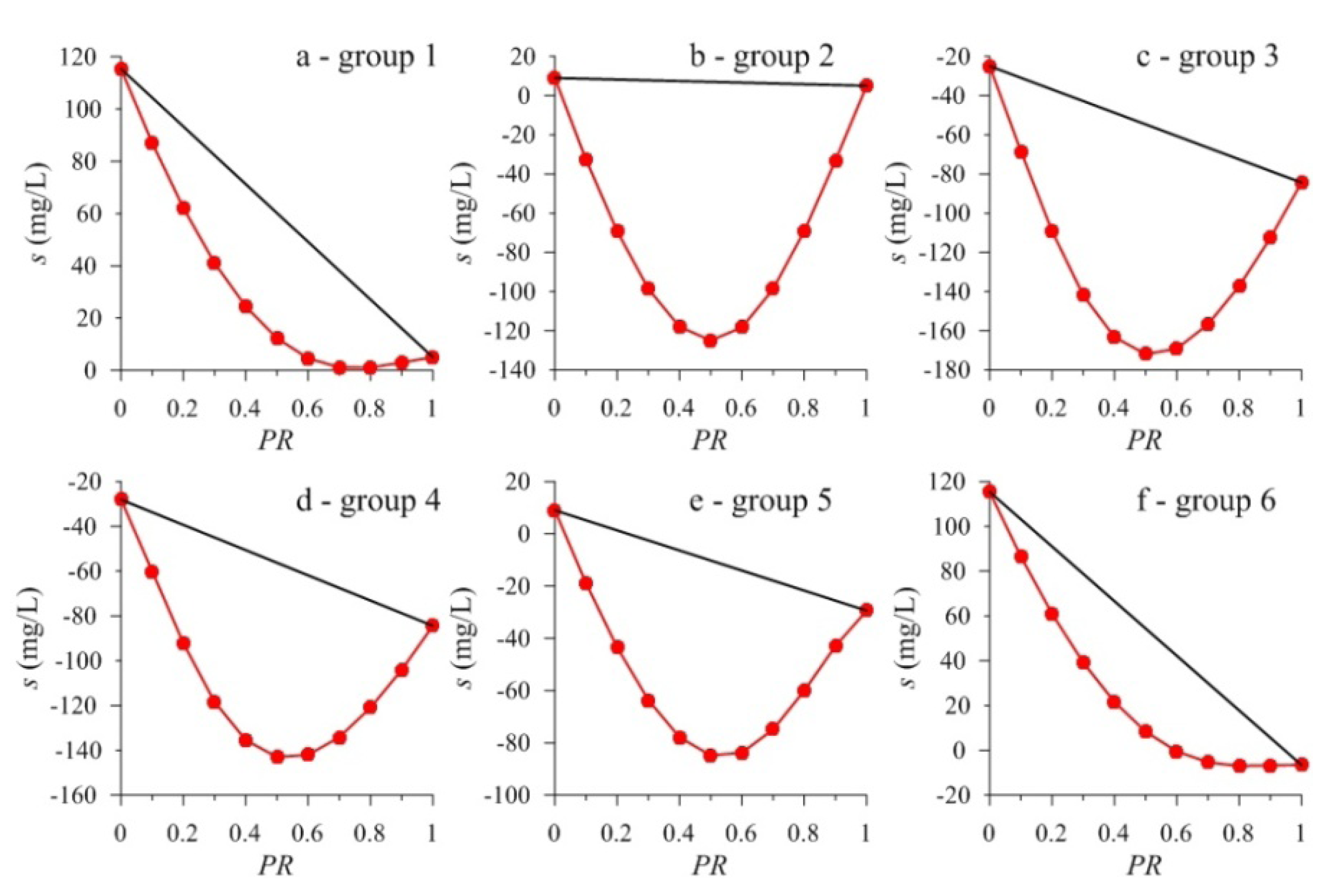
3.2.1. Mixing Precipitation between Two Unsaturated Water Samples

Group 1 and group 2 are mixed with two unsaturated water samples. The calculated results are listed in Table 3.
Table 3. Calculated results for mixed water from two unsaturated samples (group 1: water samples 1 and 2; group 2: water samples 1 and 3).
GroupItemMixing ratios
00.10.20.30.40.50.60.70.80.91.0
1pH06.506.506.516.516.526.536.546.556.576.606.65
SIc0.310.480.620.740.840.910.970.990.990.970.93
s1115.3686.9962.0641.0624.3912.264.611.141.043.005.02
s2115.36104.3393.2982.2671.2260.1949.1638.1227.0916.055.02
Δs0.00−17.34−31.23−41.20−46.83−47.93−44.55−36.98−26.05−13.050.00
pHe6.596.586.576.566.556.546.546.556.576.616.67
2pH06.806.796.796.786.786.776.766.756.736.706.65
SIc0.781.722.352.742.902.872.692.381.961.470.93
s 19.01−32.72−69.33−98.65−118.01−124.96−118.28−98.72−69.07−33.045.02
s 29.018.618.217.817.417.026.626.225.825.425.02
Δ s0.00−41.33−77.54−106.46−125.42−131.98−124.90−104.94−74.89−38.460.00
pHe6.816.766.726.676.636.596.576.566.576.606.67
Notes: pH0 and SIc are calculated pH values and saturation indices of CaCO3 for mixed waters, respectively; s1 (mg/L) is the calculated solubility (precipitability) of CaCO3 for mixed waters; s2 (mg/L) is the dissolution or precipitation amount of CaCO3 for mixed waters under no mixing precipitation assumption; Δs =s1s2; and pHe is the calculated pH values for mixed waters after solubility (precipitability) of s1.
It can be seen from Table 3 that Δs are all negative because of mixing effects, the solubility of mixed waters decreased. In other words, the mixing precipitation takes place during the mixing process. For example, for group 1 (Figure 1a), the solubility of CaCO3 in the mixed water was 62.06 mg/L at the mixing ratio of 0.2 (mixture of 0.2 L water sample 1 and 0.8 L water sample 2). However, using the calculated solubility of water samples 1 and 2 in Table 3, if they were not mixed, the total dissolution of 0.2 L of water sample 1 and 0.8 L water sample 2 should be 93.29 mg/L (0.2 × 5.02 mg/L + 0.8 × 115.36 mg/L = 93.29 mg/L). Therefore, the dissolution amount of CaCO3 was decreased by 31.23 mg/L under the mixing precipitation effect. Similarly, when the mixing ratios were 0.5 and 0.8, the decreases of CaCO3 solubility were 47.93 mg/L and 26.05 mg/L, respectively. However, the mixing effect does not change CaCO3 from the state of dissolution to precipitation in all mixing ratios. Another thing which should be stressed is that both the mixing and subsequent dissolution (precipitation) of CaCO3 change the pH of the solution. The column pH0 in Table 3 shows the pH values of mixed waters before CaCO3 dissolution (precipitation). The figures for pHe are the pH values after s1 (mg/L) of CaCO3 is dissolved (precipitated) into (from) the mixed waters. It can be seen from group 1 that the pHe is greater than pH0, which indicates that the dissolution of CaCO3 will increase the pH values of solution and can be explained by the following reactions:
Water 05 01712 i019
Water 05 01712 i020
Water 05 01712 i021
The dissolution of CaCO3 caused the concentration of H+ to decrease, which increased the pH values of the mixed water in group 1 after the dissolution of CaCO3 as a result.
According to the above discussion, a new concept, mixing precipitation in a broad sense, can be proposed. This refers to the mixing effect that causes the solubility of CaCO3 to decrease in mixed water and does not change the dissolution states of CaCO3 at the same time. Correspondingly, the mixing effect which changes the state of CaCO3 from dissolution to precipitation, or increases the precipitability of CaCO3 in mixed water is named mixing precipitation in a strict sense.
The mixing between two unsaturated samples can also lead to mixing precipitation in a strict sense. Group 2 is such an example, which is mixed by water samples 1 and 3 (Figure 1b). Before mixing, the solubility of CaCO3 in sample 1 and 3 were 5.02 and 9.01 mg/L, respectively. However, when water samples 1 and 3 were mixed at the ratio of 0.2, the mixed water produced 69.33 mg/L of CaCO3 precipitation instead. Similarly, when the mixing ratio was 0.5, the solubility of CaCO3 in mixed water should be 7.02 mg/L if there was no mixing precipitation, whereas the mixing process produced 124.96 mg/L of CaCO3 precipitation instead. When the mixing ratio was 0.8, the precipitation amount of CaCO3 caused by mixing precipitation was 69.07 mg/L. The pHe values are less than the pH0 in group 2. This is because the mixing process precipitated some CaCO3 from the water and the concentration of H+ increased in the solution.

3.2.2. Mixing Precipitation between Two Oversaturated Water Samples

Groups 3 and 4 were mixed with two oversaturated water samples. The solubility (precipitation) of CaCO3 at different mixing ratios are listed in Table 4.
It can be seen from Table 4 and Figure 1 (Figure 1c and Figure 1d) that mixing precipitation in a strict sense was observed in groups 3 and 4. In group 3, when the mixing ratio was 0.2, 109.24 mg/L of CaCO3 precipitation was formed in the mixed water, whereas if there was no mixing precipitation, only 36.858 mg/L of CaCO3 should be precipitated at the same mixing ratio. In other words, the mixing effect increased 72.38 mg/L of CaCO3 precipitation. When the mixing ratio was 0.5 and 0.8, the increased amounts of CaCO3 precipitation were 117.27 and 64.698 mg/L with mixing precipitation, respectively. In group 4, the increased amounts of CaCO3 precipitation were relatively less than those in group 3. When the mixing ratios were 0.2, 0.5 and 0.8, the mixed waters produced 52.93, 86.79 and 47.83 mg/L of CaCO3 precipitation, respectively.
Because the two end member samples were all oversaturated, the mixing precipitation in a strict sense can be only obtained from the mixed waters.
Table 4. Calculated results for mixed water from two oversaturated samples (group 3: water samples 4 and 5; group 4: water samples 4 and 6).
GroupItemMixing ratios
00.10.20.30.40.50.60.70.80.91.0
3pH07.007.027.027.027.027.027.017.017.017.007.00
SIc1.602.473.223.834.324.654.834.854.684.313.72
s1−24.97−68.42−109.24−141.95−163.23−171.96−169.14−156.73−137.22−112.62−84.41
s2−24.97−30.91−36.86−42.80−48.75−54.69−60.63−66.58−72.52−78.47−84.41
Δ s0.00−37.51−72.38−99.15−114.48−117.27−108.51−90.15−64.70−34.150.00
pHe6.866.776.736.716.726.756.786.816.856.886.92
4pHo7.257.167.127.097.077.057.047.027.027.017.00
SIc2.072.613.123.563.914.164.324.364.294.083.72
s1−28.08−60.13−92.28−118.38−135.48−143.03−142.04−134.11−120.97−104.07−84.41
s2−28.08−33.71−39.35−44.98−50.61−56.25−61.88−67.51−73.14−78.78−84.41
Δ s0.00−26.42−52.93−73.40−84.87−86.79−80.16−66.60−47.83−25.290.00
pHe7.016.896.836.806.806.816.836.856.876.906.92
Notes: pH0 and SIc are calculated pH values and saturation indices of CaCO3 for mixed waters, respectively; s1 (mg/L) is the calculated solubility (precipitability) of CaCO3 for mixed waters; s2 (mg/L) is the dissolution or precipitation amount of CaCO3 for mixed waters under no mixing precipitation assumption; Δs = s1s2; and pHe is the calculated pH values for mixed waters after solubility (precipitability) of s1.

3.2.3. Mixing Precipitation between an Unsaturated Water Sample and an Oversaturated Water Sample

Group 5 was obtained by mixing samples 3 and 8, and group 6 was mixed with samples 2 and 7. The mixing precipitation between an unsaturated sample and an oversaturated sample were calculated using the aforementioned model. The results are listed in Table 5.
For group 5 when the mixing ratio was less than or equal to 0.2, mixing precipitation in a broad sense can be observed. The state of CaCO3 changes from dissolution to precipitation under the mixing effect. For example, when the mixing ratio was 0.1, if there was no mixing precipitation, 5.17 mg/L of CaCO3 should be dissolved in the mixed water. However, under the influence of the mixing precipitation18.93 mg/L of CaCO3 was precipitated from the mixed water. This is the type of mixing precipitation which changes the states of CaCO3 from dissolution into precipitation; it is a kind of mixing precipitation in a strict sense. When the mixing ratio was larger than 0.2, the precipitation amount of CaCO3 was increased by the mixing precipitation effect. When the mixing ratio was 0.8, for instance, the mixing effects increased the precipitability of CaCO3 by an amount of 38.29 mg/L.
The phenomena in group 6 are different from those in group 5. When the mixing ratio was less than or equal to 0.5, the mixing precipitation in a broad sense occurs. The mixing effect only reduced the solubility of CaCO3, it did not change the saturation state of CaCO3. When the mixing ratio was larger than or equal to 0.6, the mixing effect changed the state of CaCO3 from dissolution to precipitation, thus, mixing precipitation in a strict sense occurs. For example, when the mixing ratio was 0.3, if there is no mixing precipitation, 78.78 mg/L of CaCO3 will be dissolved in the mixed water, but because of the impact of mixing precipitation, only 38.16 mg/L of CaCO3 dissolved. When the mixing ratio is 0.8, 17.82 mg/L of CaCO3 can be dissolved in the mixed water under the assumption of no mixing precipitation, but under the influence of mixing precipitation, 7.01 mg/L of CaCO3 is precipitated instead. In this case, mixing precipitation in a strict sense occurs.
Table 5. Calculated results for mixed water from an unsaturated sample and an oversaturated sample (group 5: water samples 3 and 8, group 6: water samples 2 and 7).
GroupItemMixing ratios
00.10.20.30.40.50.60.70.80.91.0
5pH06.806.816.816.836.846.866.896.926.977.067.26
SIc0.781.421.872.152.312.362.322.222.091.972.16
s19.01−18.93−43.54−63.65−77.87−84.83−83.75−74.85−60.03−42.89−29.43
s29.015.171.32−2.52−6.37−10.21−14.05−17.90−21.74−25.59−29.43
Δs0.00−24.10−44.86−61.13−71.50−74.62−69.70−56.95−38.29−17.300.00
pHe6.816.796.776.756.736.736.736.756.796.877.01
6pHo6.506.516.516.526.536.546.556.576.596.646.71
SIc0.310.480.620.750.860.941.001.051.071.081.11
s1115.3686.4760.9439.1621.608.36−0.51−5.35−7.01−6.69−6.57
s2115.36103.1790.9778.7866.5954.4042.2030.0117.825.62−6.57
Δs0.00−16.70−30.03−39.62−44.99−46.04−42.71−35.36−24.83−12.310.00
pHe6.596.586.576.566.556.556.556.566.586.626.68
Notes: pH0 and SIc are calculated pH values and saturation indices of CaCO3 for mixed waters, respectively; s1 (mg/L) is the calculated solubility (precipitability) of CaCO3 for mixed waters; s2 (mg/L) is the dissolution or precipitation amount of CaCO3 for mixed waters under no mixing precipitation assumption; Δs =s1s2; and pHe is the calculated pH values for mixed waters after solubility (precipitability) of s1.
It can be concluded that when an unsaturated water sample and an oversaturated water sample are mixed, the mixing precipitation both in a strict sense and in a broad sense can be produced. Which of these phenomena occurs depends on the hydrochemical characteristics of the end member solutions and the saturation states before and after mixing.

3.2.4. General Characteristics of End Member Samples for Mixing Precipitation

The above analyses and discussions illustrate that mixing precipitation is a common phenomenon in natural waters. It can be produced by mixing between two supersaturated water samples, between two unsaturated water samples or between an unsaturated water sample and an oversaturated water sample. The mixing precipitation in a strict sense can be observed in all three mixing types, while the mixing precipitation in a broad sense cannot be produced by mixing between two oversaturated samples. Therefore, it can be concluded that mixing precipitation in a broad sense can only be observed when at least one of the end member solutions is unsaturated, and the solubility or precipitability of CaCO3 is controlled by the saturation index in mixed water. Besides, the mixing precipitation is also influenced by the hydrochemical characteristics of end member solutions. A large number of calculations reveal that if mixing precipitation (including mixing precipitation in strict sense and in broad sense) occurs, the two end member aqueous solutions generally possess the following characteristics: when the HCO3 concentration in one aqueous solution is higher than that in the other solution, the concentration of Ca2+ in the former aqueous solution is usually lower than that in the latter. That is to say, when two water samples are mixed, if one solution contains a large amount of HCO3 and the other contains a lot of Ca2+, mixing precipitation of CaCO3 will occur when they are mixed.

4. Conclusions

According to the discussions above, the following conclusions can be derived:
(1) Precipibility (Solubility) can be calculated based on a chemical equilibrium model for mixed waters considering mixing precipitation. The calculated results show that mixing precipitation can be classified into two major types: mixing precipitation in a strict sense and mixing precipitation in a broad sense. Mixing precipitation in a strict sense refers to the effect that makes the state of CaCO3 change from dissolution to precipitation, or increases the precipitability of CaCO3. Mixing precipitation in a broad sense refers to the mixing effect that reduces the solubility of CaCO3.
(2) Mixing precipitation is a common phenomenon in natural waters system. It can be observed by mixing between two unsaturated water samples, two oversaturated water samples, or an unsaturated and an oversaturated sample. Mixing precipitation in a broad sense cannot be observed when two oversaturated samples are mixed.
(3) The mixing precipitation is controlled by the simultaneous chemical equilibria that are established, which can be expressed in terms of saturation indices of the end member solutions and influenced by their hydrochemical characteristics. Generally, if the HCO3 concentration is higher in one solution and the Ca2+ concentration is higher in the other, mixing precipitation of CaCO3 will be produced when they are mixed.

Acknowledgments

The research was supported by the National Natural Science Foundation of China (41172212), the Doctoral Postgraduate Technical Project of Chang’an University (2013G5290002 and CHD2011ZY022) and the special Fund for Basic Scientific Research of Central Colleges, Chang’an University (CHD2012TD003).

Conflicts of Interest

The authors declare no conflict of interest.

References

  1. Crandall, C.A.; Katz, B.G.; Hirten, J.J. Hydrochemical evidence for mixing of river water and groundwater during high-flow conditions, lower Suwannee River basin, Florida, USA. Hydrogeol. J. 1999, 7, 454–467. [Google Scholar] [CrossRef]
  2. Doria, M.F.; Pidgeon, N.; Hunter, P.R. Perceptions of drinking water quality and risk and its effect on behaviour: A cross-national study. Sci. Total Environ. 2009, 407, 5455–5464. [Google Scholar] [CrossRef]
  3. Inoue, R.; Yoshida, J.; Hiroe, Y.; Komatsu, K.; Kawasaki, K.; Yasuda, I. Modification of North Pacific intermediate water around mixed water region. J. Oceanogr. 2003, 59, 211–224. [Google Scholar] [CrossRef]
  4. Mao, B.Y.; Xu, M.; Zhong, B.A.; Huang, R.Y. Study on the karst development law and mechnism HESAN Coal Field Guangxi. Res. Soil Water Conserv. 2007, 14, 137–140. (in Chinese). [Google Scholar]
  5. Paulsen, S.; List, E.J. A study of transport and mixing in natural waters using ICP−MS: Water-particle interactions. Water Air Soil Poll. 1997, 99, 149–156. [Google Scholar]
  6. Gong, Z.Z. Mixing corrosion tests of natrual water in Guilin karst region. Carsologica Sinica 1987, 6, 245–254. (in Chinese). [Google Scholar]
  7. Huang, F.; Tang, W.; Wang, J.M.; Cao, J.H.; Yin, J.J. The influence of allogenic water on karst carbon sink: A case study in the Maocum Subterranean River in Guilin, China. In Carsologica Sinica; 2011; Volume 30, pp. 417–421. (in Chinese) [Google Scholar]
  8. Rygaard, M.; Arvin, E.; Binning, P.J. The valuation of water quality: Effects of mixing different drinking water qualities. Water Res. 2009, 43, 1207–1218. [Google Scholar] [CrossRef]
  9. Shen, H.T.; Zhang, C.L. Mixing of salt water and fresh water in the Changjiang River estuary and its effects on suspended sediment. Chin. Geogr. Sci. 1992, 2, 373–381. [Google Scholar] [CrossRef]
  10. Bögli, A. Karst Hydrology and Physical Speleology; Springer Verlag: Berlin, Germany, 1980; pp. 1–284. [Google Scholar]
  11. Chen, H.H.; Zou, S.Z.; Zhu, Y.F.; Chen, CX. An experimental study of mixture corrosion effects of carbonate rocks in the transitional zone of littoral karst areas. Acta Geol. Sinica 2001, 75, 298–302. [Google Scholar]
  12. Ramos-Leal, J.A.; Martínez-Ruiz, V.J.; Rangel-Mendez, J.R.; Alfaro de la Torre, M.C. Hydrogeological and mixing process of waters in aquifers in arid regions: A case study in San Luis Potosi Valley, Mex. Environ. Geol. 2007, 53, 325–337. [Google Scholar] [CrossRef]
  13. Zou, S.Z.; Zhu, Y.F.; Chen, H.H.; Wang, C.K. Chemistry process of seawater in littoral karst area of Daweijia, Dalian city. Mar. Geol. Quat. Geol. 2004, 24, 61–68. (in Chinese). [Google Scholar]
  14. Qian, H.; Li, P.Y. Mixing corrosion of CaCO3 in natural waters. E J. Chem. 2011, 8, 1124–1131. [Google Scholar] [CrossRef]
  15. Kaufmann, G. Numerical models for mixing corrosion in natural and artificial karst environments. Water Resour. Res. 2003, 39, 1157–1168. [Google Scholar] [CrossRef]
  16. Dreybrodt, W. Kinetics of the dissolution of calcite and its applications to karstification. Chem. Geol. 1980, 31, 245–269. [Google Scholar] [CrossRef]
  17. Dreybrodt, W. Mixing corrosion in CaCO3/1bCO2/1bH2O systems and its role in the karstification of limestone areas. Chem. Geol. 1981, 32, 221–236. [Google Scholar] [CrossRef]
  18. Qian, H.; Li, P.Y. Proportion dependent mixing effects of CaCO3 in natural waters. Asian J. Chem. 2012, 24, 2257–2261. [Google Scholar]
  19. Tong, W.; Zhang, M.; Zhang, Z.; Liao, Z.; You, M.; Zhu, M.; Guo, G.; Liu, S. Geothermal Resources in Tibet; (in Chinese). Science Press: Beijing, China, 1981; pp. 24–57. [Google Scholar]
  20. Crerar, D.A. A method for computing multicomponent chemical equilibria based on equilibrium constants. Geochim. Cosmochim. Acta 1975, 39, 1375–1384. [Google Scholar] [CrossRef]
  21. Qian, H. A calculation method of the possible distribution of the dissolved species and the Eh values in aqueous solution. J. Xi'an Coll. Geol. 1987, 9, 69–80. (in Chinese). [Google Scholar]
  22. Arnórsson, S.; Sigurdsson, S.; Svavarsson, H. The chemistry of geothermal waters in Iceland. I. calculation of aqueous speciation from 0° to 370°. Geochim. Cosmochim. Acta 1982, 46, 1513–1532. [Google Scholar] [CrossRef]
  23. Qian, H.; Zhang, X.D.; Li, P.Y. Calculation of CaCO3 solubility (precipitability) in natural waters. Asian J. Chem. 2012, 24, 668–672. [Google Scholar]
  24. Plummer, L.N.; Parkhurst, D.L.; Kosiur, D.R. MIX2: A Computer Program for Modeling Chemical Reactions in Natural Waters; U.S. Department of the Interior, Geological Survey: Reston, VA, USA, 1975; pp. 1–70. [Google Scholar]
  25. Qian, H.; Song, X.; Zhang, X.D.; Yang, C.; Li, P.Y. Calculation of PH values for mixed waters. E J. Chem. 2011, 8, 657–664. [Google Scholar] [CrossRef]

