Numerical Investigation on the Hydrodynamic Coefficients of Subsea Suspended Pipelines Under Unidirectional Currents

Abstract

Hydrodynamic coefficients of subsea suspended pipelines are crucial for fatigue and stability assessments. The effect of the gap height to diameter ratio e/D (0.1 ≤ e/D ≤ 2.0) and boundary layer thickness to diameter ratio δ/D (0.5 ≤ δ/D ≤ 3.0) on the force coefficients under unidirectional current conditions with the Reynolds numbers Re in the range of 1 × 10⁴ ≤ Re ≤ 1 × 10⁵ are investigated via numerical simulations. The results show that the average drag coefficient increases, whereas the average lift coefficient decreases gradually with the increasing e/D. The vortex shedding is inhibited by the wall for e/D < 0.24, starts at e/D = 0.24, becomes stronger with the increase in e/D in the range from 0.24 to 0.5, and approximates to that behind a wall-free cylinder for e/D > 0.5. The effect of δ/D can be eliminated if the coefficients are normalized by the undisturbed flow velocity at the height of the center of the pipeline. Moreover, empirical prediction formulas are proposed describing the drag and lift coefficients as the function of e/D, which can be applied to engineering designs related to free spans.

1. Introduction

Subsea pipelines, serving as critical infrastructures connecting onshore terminals to offshore oil production platforms, play a vital role in transporting oil and gas resources and are often referred to as the lifelines of offshore energy transportation. Free spans usually occur due to local scour around subsea pipelines and the hydrodynamic forces acting on the free spans are crucial for the in situ stability (DNV [1]) and long-term operational safety of the pipelines (DNV [2]).

Under current conditions, the governing parameters for the hydrodynamic forces on a spanning pipeline are the gap ratio and the Reynolds number. The gap ratio is defined as e/D, where e is the distance from the lower surface of the pipeline to the seabed, and D is the pipeline diameter. Although the development process of the local scour is three-dimensional, the scour hole is regarded as two-dimensional, and the hydrodynamic forces are usually deemed uniform along the span in engineering designs, as demonstrated by Liang et al. [3]. When the local scour reaches an equilibrium state, the gap ratio is approximately 1.0. The Reynolds number is defined as Re = u₀D/υ, where u₀ is the free stream velocity outside the boundary layer of the incoming flow, and υ is the water kinematic viscosity. The hydrodynamic forces acting on a pipeline can be divided into the drag force F_D and the lift force F_L, and they can be further quantified as the sum of the time-mean value and the r.m.s value, respectively. The force coefficients corresponding to the time-mean and r.m.s. values are written as C_D, C_Drms for the drag force and C_L, C_Lrms for the lift force.

Kiya [4] and Roshko et al. [5] conducted physical experiments to study the effect of e/D on the time-mean drag force coefficient C_D when Re were in the range of 1 × 10⁴~4 × 10⁴ and equal to 2 × 10⁴, respectively. Kiya’s [4] results show that the C_D increases with the increase in the e/D until it remains constant after e/D increases to a critical value of about 0.4~0.5. However, Roshko’s results [5] indicate that the critical value of the gap ratio beyond which the drag force coefficient remains constant is influenced by the incoming flow boundary layer thickness δ. Further, Lei et al. [6] studied the effect of the δ/D and e/D on the hydrodynamic coefficients of a circular cylinder via physical experiments, with Re ranging from 1.30 × 10⁴ to 1.45 × 10⁴. By laying round rods close to the seabed at the far end of the incoming flow, Lei et al. [6] altered the height of the seabed roughness and yielded different thicknesses of the incoming flow boundary layer (0.14 ≤ δ/D ≤ 2.89). Their experimental results show that C_D increases with the increase in e/D when e/D ≤ 0.6; when e/D > 0.6, C_D almost remains constant. However, C_D was demonstrated to be affected by the ratio of δ/D. It should be noted that in the research work of Lei et al. [6], the force coefficients are normalized with u₀. The experiments conducted by Zdrakovick [7] also demonstrate that the force coefficients are variant with δ/D. Most recently, Teng et al. [8] investigated the effect of the velocity gradient in the boundary layer on the time-mean force coefficients. Their results show that the force coefficients deviate significantly when different boundary layer properties are introduced.

In addition to physical experiments, many researchers have also studied the influence of different parameters on the hydrodynamic coefficients of circular cylinders through numerical simulations. Brørs [9] established a numerical model for the forces acting on pipelines that can consider the influence of local scouring topography by using the Reynolds-averaged N–S equations combined with the k-ε turbulence closure model. The relevant numerical calculation results show that when e/D = 1.0 and Re = 1.5 × 10⁴, the average values of the drag force and lift force coefficients calculated by using the two-dimensional numerical analysis model agree well with the experimental results. Kazeminezhad et al. [10] used a numerical model similar to that of Brørs [9] to obtain the hydrodynamic coefficients of the pipeline within the parameter ranges of Re = 9500, 0 ≤ e/D ≤ 2.0, and 0.3 ≤ δ/D ≤ 3.0. The results show that when the boundary layer thickness is the same, the variation trends of the average drag force coefficient and the average lift force coefficient with the gap ratio are consistent with the results of physical experiments.

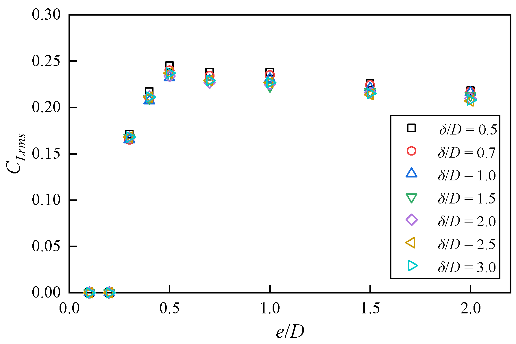
The r.m.s. force coefficients are related to vortex shedding in the wake of the pipeline. Lei et al. [11] investigated the influence of the Reynolds number (Re = 80~10³) and the gap ratio (0.1 ≤ e/D ≤ 3.0) on the flow structure around a pipeline and the forces acting on it by solving the two-dimensional Navier–Stokes (N–S) equations. Their results show that the critical gap ratio for the onset of vortex shedding is approximately 0.2. Ong et al. [12] used the two-dimensional Reynolds-averaged N–S equations combined with the k-ε turbulence closure model to study the mechanism of vortex shedding from a near-wall circular cylinder when Re = 1.31 × 10⁴ and in the range of 0.1 ≤ e/D ≤ 1.0. Their results show that the vortex structure is inhibited by the wall when the gap ratio e/D ≤ 0.3. However, the effect of δ/D on C_Drms and C_Lrms has not been well investigated.

All the above justifications suggest that an additional parameter noticeably affects the hydrodynamic forces, namely, the boundary layer thickness to diameter ratio δ/D. However, empirical methods for evaluating the force coefficients under the effect of δ/D have not been proposed. Therefore, this study takes the forces acting on the subsea suspended pipeline as the research object, focuses on analyzing the influence of the thickness of the incoming flow boundary layer and the pipeline gap ratio on the forces acting on the pipeline, and aims to establish an empirical prediction method for the hydrodynamic coefficients of the suspended pipeline under the action of unidirectional flow, so as to provide a scientific basis and technical reference for the safety design, operation, and maintenance of the pipeline.

2. Materials and Methods

The numerical simulations in this study were carried out using the open-source software OpenFOAM-10. The fluid flow control equations are the continuity equation and the Reynolds-averaged Navier–Stokes (N–S) equations for two-dimensional incompressible viscous fluids. In the Cartesian coordinate system, the governing equations are as follows:

$${\displaystyle \frac{\partial u_i}{\partial x_i}}=0$$

(1)

$${\displaystyle \frac{\partial u_i}{\partial t}}+u_j{\displaystyle \frac{\partial u_i}{\partial x_j}}=-{\displaystyle \frac{1}{\rho }}{\displaystyle \frac{\partial p}{\partial x_i}}+{\displaystyle \frac{\partial }{\partial x_j}}\left(2\upsilon S_{ij}-\overline{u_i^{’}{u}_j^{’}}\right)$$

(2)

Among them, x₁ = x and x₂ = y are the coordinate components in the Cartesian coordinate system, u_i is the ith velocity component with respect to the coordinate x_i (u₁ = u and u₂ = v correspond to x₁ = x and x₂ = y, respectively), t is the time, ρ is the fluid density, p is the pressure, and ν is the kinematic viscosity of the fluid. S_ij = (∂u_i/∂x_j + ∂u_j/∂x_i)/2 represents the strain-rate tensor. $\overline{u_i^{’}{u}_j^{’}}$ is the Reynolds stress, and its calculation formula is

$$\overline{u_i^{’}{u}_j^{’}}=-{\upsilon }_t\left(\partial u_i/\partial x_j+\partial u_j/\partial x_i\right)+{\displaystyle \frac{2}{3}}k{\delta }_{ij}$$

(3)

In the above formula, k is the turbulent kinetic energy, and δ_ij is the Kronecker operator.

The Reynolds stress term $\overline{u_i^{’}{u}_j^{’}}$ makes the above-mentioned control equations unclosed. Therefore, a turbulence model needs to be introduced to close and solve the equations. In the present study, the SST k − ω two-equation turbulent model proposed by Menter [13] and Menter et al. [14] is employed. The corresponding control equations consist of the turbulent kinetic energy k and the kinetic energy dissipation rate ω, and their forms are as follows:

$${\displaystyle \frac{\partial k}{\partial t}}+u_j{\displaystyle \frac{\partial k}{\partial x_j}}={\displaystyle \frac{\partial }{\partial x_j}}\left[\left(\upsilon +{\sigma }_k{\upsilon }_t\right){\displaystyle \frac{\partial k}{\partial x_j}}\right]+p_k-{\beta }^{\ast }\omega k$$

(4)

$${\displaystyle \frac{\partial \omega }{\partial t}}+u_j{\displaystyle \frac{\partial \omega }{\partial x_j}}={\displaystyle \frac{\partial }{\partial x_j}}\left[\left(\upsilon +{\sigma }_{\omega }{\upsilon }_t\right){\displaystyle \frac{\partial \omega }{\partial x_j}}\right]+{\displaystyle \frac{\alpha p_k}{{\upsilon }_t}}-\beta {\omega }^2+2\left(1-F_1\right){\sigma }_{\omega 2}{\displaystyle \frac{1}{\omega }}{\displaystyle \frac{\partial k}{\partial x_j}}{\displaystyle \frac{\partial \omega }{\partial x_j}}$$

(5)

In the above formulae, p_k is the generation of turbulent kinetic energy, υ_t is the turbulent eddy viscosity, and F₁ is the blending function. They can be expressed as follows:

$$p_k=\min \left[{\upsilon }_t{\displaystyle \frac{\partial u_i}{\partial x_j}}\left({\displaystyle \frac{\partial u_i}{\partial x_j}}+{\displaystyle \frac{\partial u_j}{\partial x_i}}\right),10{\beta }^{\ast }k\omega \right]$$

(6)

$${\upsilon }_t={\displaystyle \frac{{\alpha }_{1}k}{\max \left({\alpha }_1\omega ,S{F}_2\right)}}$$

(7)

$$F_1=\tanh \left\{\left.\left\{{\left.\min \left[\max \left({\displaystyle \frac{\sqrt{k}}{{\beta }^{*}\omega y*}},{\displaystyle \frac{500\upsilon }{y{*}^2\omega }}\right), {\displaystyle \frac{4\rho {\sigma }_{\omega 2}k}{D_{k\omega }y{*}^2}}\right]\right\}}^4\right.\right\}\right.$$

(8)

In the formulas, S = (2S_ijS_ij)^1/2 is the invariant measure of the strain rate, y⁺ is the dimensionless distance from the nearest grid to the wall surface, and the variables F₂ and D_kω are expressed as

$$F_2=\tanh \left\{{\left[\max \left({\displaystyle \frac{2\sqrt{k}}{{\beta }^{*}\omega y*}},{\displaystyle \frac{500\upsilon }{y{*}^2\omega }}\right)\right]}^2\right\}$$

(9)

$$D_{k\omega }=\max \left(2\rho {\sigma }_{\omega 2}{\displaystyle \frac{1}{\omega }}{\displaystyle \frac{\partial k}{\partial x_j}}{\displaystyle \frac{\partial \omega }{\partial x_j}},{10}^{-10}\right)$$

(10)

Based on the blending function F₁, σ_k = F₁σ_k1 + (1 − F₁)σ_k2, σ_ω = F₁σ_ω1 + (1 − F₁)σ_ω2, α = F₁α₁ + (1 − F₁)α₂, and β = F₁β₁ + (1 − F₁)β₂. The coefficients of the SST k − ω turbulent model used in Equations (4)–(10) are shown in

Table 1. Parameters in the SST k-ω turbulence model.

β*	α1	β1	σk1	σω1	α2	β2	σk2	σω2
0.09	5/9	3/40	0.85	0.5	0.44	0.0828	1.0	0.856

:

2.1. Numerical Calculation Model

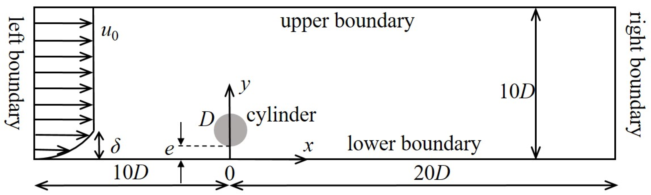
The computational domain of the two-dimensional force calculation model for a suspended pipeline under the action of unidirectional flow is presented in Figure 1. The coordinate origin is set on the seabed and below the center of the pipeline. The pipeline center is located at a distance e + D/2 above the seabed, where e is the height from the bottom of the pipeline to the seabed, with D being the pipeline diameter. To ensure that the flow structure around the pipeline is not influenced by the boundaries shown in Figure 1, the distance between the left boundary and the pipeline center is 10D, while the corresponding distance is 20D for the downstream.

The boundary conditions for the present numerical model are set as follows: For the left boundary, the boundary conditions are u = u(y), v = 0, ∂p/∂x = 0, ∂k/∂n = 0, ∂ω/∂n = 0. For the right boundary, they are ∂u/∂x = 0, ∂v/∂y = 0, p = 0, ∂k/∂n = 0, ∂ω/∂n = 0. The upper boundary is a slip boundary with u = u₀, v = 0, ∂p/∂y = 0, ∂k/∂n = 0, ∂ω/∂n = 0. Both the lower boundary and the cylinder surface are non-slip boundaries. The boundary conditions are u = 0, v = 0, ∂p/∂n = 0, ω = 6υ/0.075Δ². The boundary conditions for the turbulent kinetic energy k at the lower boundary and the cylinder surface are ∂k/∂n = 0 and k = 0, respectively. Here, ν is the kinematic viscosity of the fluid, Δ is the height of the first-layer grid from the cylinder surface, and n is the unit vector of the outer normal vector of the boundary.

To simulate the incoming flow conditions with different boundary-layer thicknesses at the inlet, within the boundary layer (y ≤ δ), the specified velocity profile satisfies the logarithmic distribution law; outside the boundary layer (y > δ), the corresponding flow velocity is the free-stream velocity u₀. The velocity distribution formula is as follows:

$$u(y)=\left\{\begin{array}{cc}\min \left\{{\displaystyle \frac{u_{*}}{\kappa }}\ln \left(y/z_w\right),u_0\right\} & y>0\\ 0& y=0\end{array}\right.$$

(11)

In the formula, u(y) represents the horizontal flow velocity at the vertical coordinate y, u_* represents the friction velocity, κ is the von Kármán constant, and κ = 0.41 is taken in the present study. z_w represents the seabed roughness length, which reflects the roughness length of the seabed. For a sandy seabed, z_w = d₅₀/12 is employed, and d₅₀ represents the median particle size of the sediment. For the subsequent numerical calculations of the present study, z_w = 1 × 10⁻⁶ m is taken.

The calculation formulas of the forces and the corresponding coefficients are written as follows:

$$F_D={\displaystyle {\int }_0^{2\pi }\left[p\cos \left(\varphi \right)+{\tau }_0\sin \left(\varphi \right)\right]}{r}_{0}d\varphi$$

(12)

$$F_L={\displaystyle {\int }_0^{2\pi }\left[p\sin \left(\varphi \right)+{\tau }_0\cos \left(\varphi \right)\right]}{r}_{0}d\varphi$$

(13)

$$C_D=2F_D/(\rho u_0^{2}D)$$

(14)

$$C_L=2F_L/(\rho u_0^{2}D)$$

(15)

In the above formulas, p represents the pressure, τ₀ is the shear stress along the surface of the pipeline, and r₀ is the radius of the pipeline, as shown in Figure 2; ρ represents the fluid density.

2.2. Grid Convergence Verification

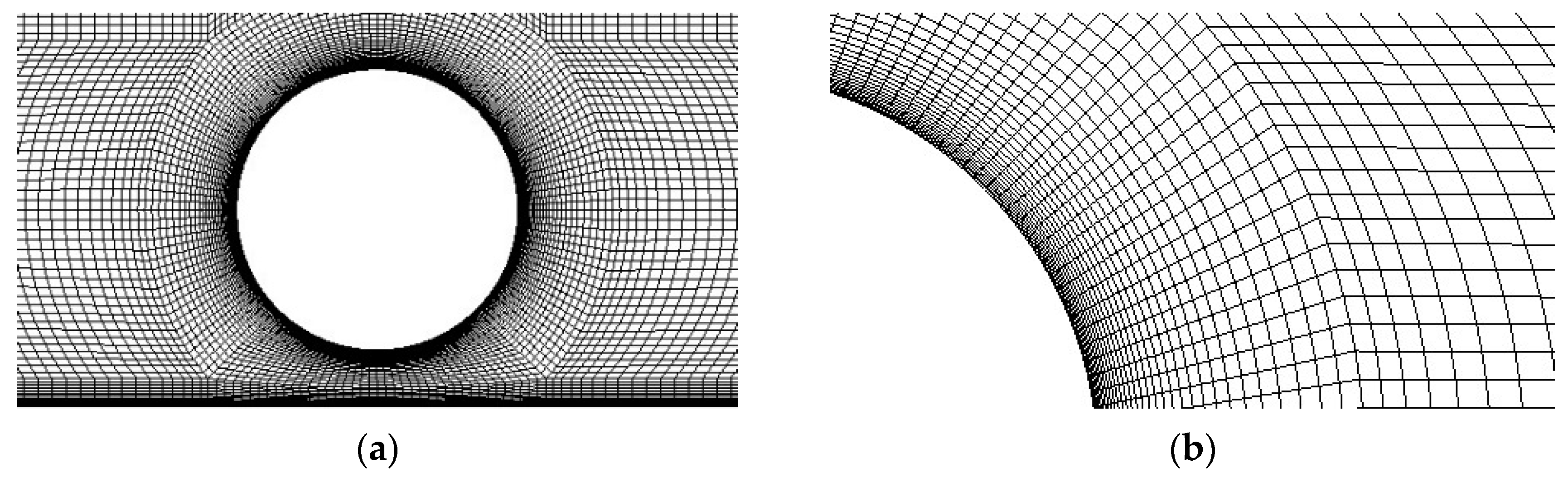
To guarantee the accuracy of the numerical model, the grid convergence is verified first before conducting the formal numerical simulations. The entire computational domain is discretized using four-node quadrilateral grids. Figure 3a shows the grids divided near the entire pipeline. There are mainly two encryption measures: one is to change the number of circumferential nodes on the pipeline surface, and the other is to change the height of the first-layer grids on the pipeline surface and the seabed. A locally enlarged view of the grid discretization around the pipeline is presented in Figure 3b.

Table 2. Mesh discretization for grid convergence verification under unidirectional flow conditions.

Mesh Number	Number of Nodes on the Pipeline Surface	Total Number of Elements	Total Number of Nodes	Height of the First Layer of Mesh on the Pipeline	CDm	CLm
G1	100	32,571	32,999	0.002D	1.173	0.167
G2	120	40,068	40,539	0.002D	1.182	0.151
G3	140	50,253	50,784	0.002D	1.271	0.124
G4	160	60,140	60,727	0.002D	1.280	0.115
G5	180	70,461	71,094	0.002D	1.286	0.118
G6	160	55,982	56,559	0.004D	1.242	0.147
G7	160	58,140	58,723	0.003D	1.273	0.118
G8	160	64,336	64,934	0.001D	1.281	0.112

presents the grid information and verification results for the convergence verification of the pipeline surface nodes (G1~G5) and the height of the first-layer surface grids (G4, G6, G7, G8). In the present study, under the conditions of Re = 1 × 10⁴, e/D = 0.5, and δ = 2D, the average drag force coefficient C_Dm and the average lift force coefficient C_Lm are compared and verified. Here, C_Dm and C_Lm are obtained by taking the time-average of the values of C_D and C_L within 30 periods after they become stable. The results show that when the number of pipeline surface nodes is 160 and the height of the first-layer grid is 0.002D, the grid meets the convergence requirements. Subsequent calculation work will be carried out according to this grid division method.

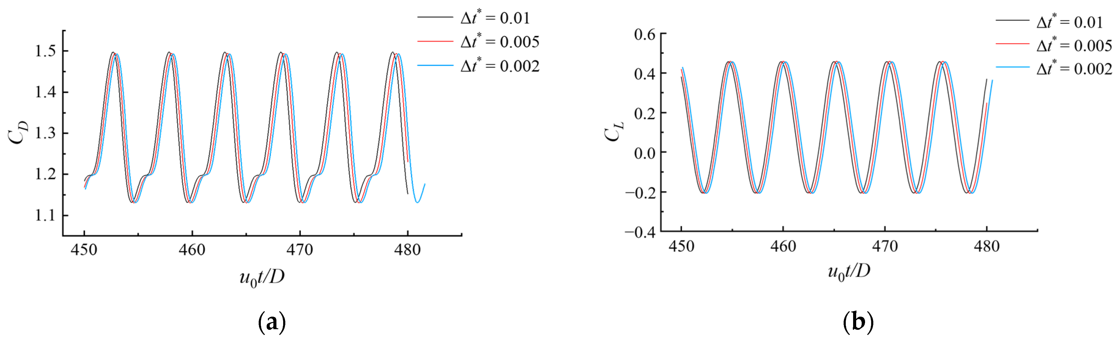
2.3. Verification of Time Step Convergence

In addition to verifying the convergence of the grid size, it is also necessary to verify the convergence of the time step. Equation (16) shows the method of dimensionless treatment for the time step:

$$\Delta t^{*}={\displaystyle \frac{u_0\Delta t}{D}}$$

(16)

Among them, Δt is the dimensional time step, and u₀ is the free stream velocity. Under the conditions of the Reynolds number Re = 1 × 10⁴, the gap ratio e/D = 0.5, and the boundary layer thickness δ = 2D, the convergence of the time steps Δt* = 0.01, 0.005, and 0.002 is verified, and the corresponding numerical results are shown in Figure 4. The oscillation of force coefficients observed in Figure 4 is related to vortex shedding.

The above results indicate that when Δt* = 0.01, the drag force coefficient is slightly larger, and its frequency also changes over time. The calculation results using Δt* = 0.005 and Δt* = 0.002 are basically the same. Therefore, Δt* = 0.005 is selected for the subsequent numerical calculations in the present study.

Employing the established numerical model in the present study, the calculated average horizontal velocity, average drag force coefficient C_Dm, average lift force coefficient C_Lm, and root mean square value of the lift force coefficient C_Lrms are compared with the experimental and numerical simulation results obtained by previous studies to examine the accuracy of the present numerical model.

First, the average horizontal velocity around the pipeline calculated under the conditions of Re = 9500, e/D = 0.2, and e/D = 0.3, and the boundary layer thickness δ = 2D is compared with the experimental results reported by Oner et al. [15]. The comparison results are shown in Figure 5, where the circles represent the experimental data of Oner et al. [15], and the red solid line represents the present numerical results.

It is seen from Figure 5 that, when the gap ratio e/D = 0.2, the present numerical results agree well with the experimental data reported by Oner et al. [15]. When the gap ratio e/D = 0.3, the average horizontal velocity of the flow field in front of the pipeline is consistent with the experimental results. Although there is a certain error between the distribution of the average horizontal velocity behind the pipeline and the experimental results, this error is within an acceptable range. Therefore, this model can accurately simulate the flow field characteristics of the flow around a cylinder.

On the basis of the above comparison and verification, the hydrodynamic force on a suspended pipeline is further verified. The calculation conditions are as follows: Re = 1 × 10⁴, e/D = 0.5, and δ = 2D. The average drag force coefficient C_Dm, average lift force coefficient C_Lm, and root mean square value of the lift force coefficient C_Lrms calculated by the present numerical model are compared with the experimental results of Jensen et al. [16] and the numerical results of Kazeminezhad et al. [10] and Tang et al [17]. The comparison results are shown in Figure 6.

As can be seen from Figure 6, the calculation results of the numerical model in the present study are very close to the experimental results reported by Jensen et al. [16] and the numerical results of Kazeminezhad et al. [10] and Tang et al. [17], which fully demonstrates that this model can accurately simulate the force-bearing characteristics of the flow around a cylinder under the action of unidirectional flow.

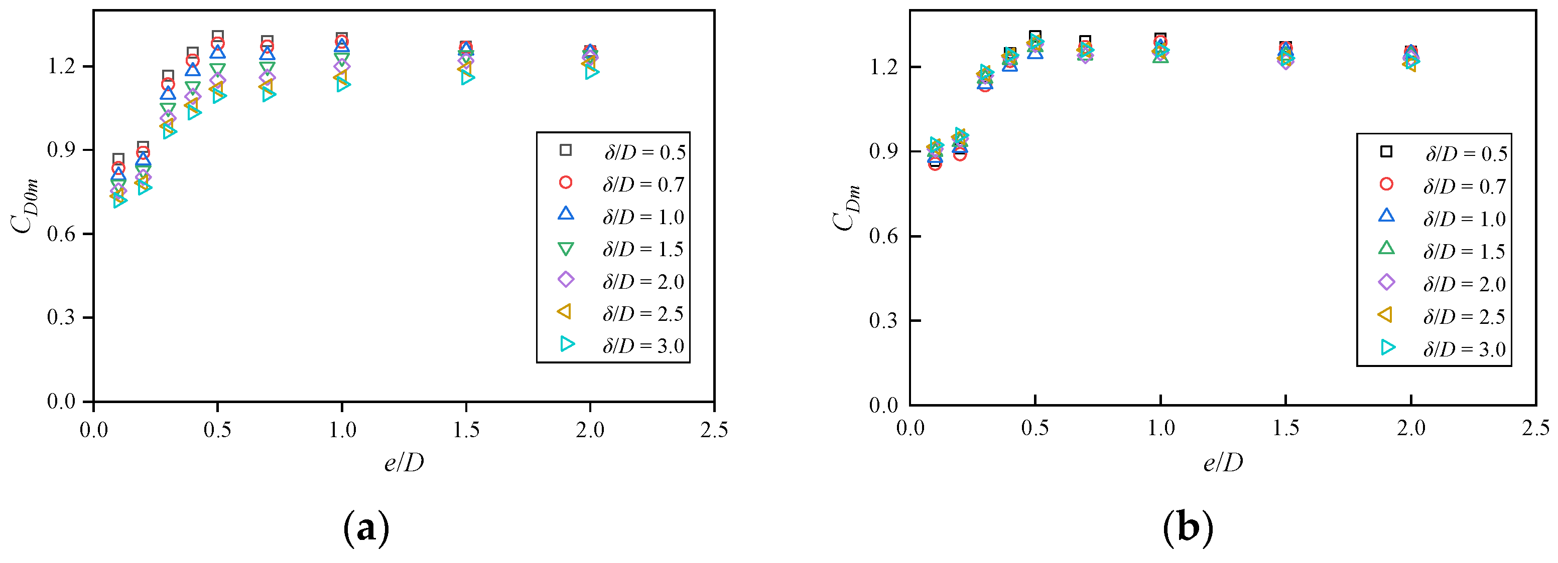
2.4. Summary of Simulations

The parameter settings for the numerical calculation are as follows: The Reynolds number Re = 1 × 10⁴, the gap ratios e/D = 0.1, 0.2, 0.3, 0.4, 0.5, 0.7, 1.0, 1.5, and 2.0, and the thicknesses of the incoming flow boundary layer δ/D = 0.5, 0.7, 1.0, 1.5, 2.0, 2.5, and 3.0. In the numerical simulations, the effects of the boundary layer thickness δ/D and the gap ratio e/D on the hydrodynamic force acting on the pipeline and the vortex shedding frequency are analyzed in the next section.

3. Numerical Results and Discussion

3.1. Average Values of the Drag Force Coefficient and the Lift Force Coefficient

As known from the previous analysis, in the early research works, the free stream velocity u₀ was employed to make the hydrodynamic force acting on the pipeline dimensionless to obtain the hydrodynamic coefficients. However, this method is greatly affected by the thickness of the boundary layer. Therefore, in this section, the free stream velocity u₀ and the flow velocity u_a at the height of the middle of the pipeline (the flow is simulated without the presence of the pipeline) are used, respectively, to make the hydrodynamic force dimensionless. The calculation formulas of the hydrodynamic coefficients obtained from the dimensionless analysis are shown in Equations (14) and (15). The hydrodynamic coefficients of the pipeline obtained by making the force dimensionless with the flow velocity u_a at the center of the pipeline diameter are shown in Equations (17) and (18):

$$C_D=2F_D/(\rho u_a^{2}D)$$

(17)

$$C_L=2F_L/(\rho u_a^{2}D)$$

(18)

Compare the hydrodynamic coefficients after the two kinds of dimensionless treatments, and analyze the influences of the non-dimensional boundary layer thickness δ/D and the gap ratio e/D on the average drag force coefficient and the average lift force coefficient. The specific results are shown in Figure 7 and Figure 8. It should be noted that, in order to distinguish the hydrodynamic coefficients obtained by the two dimensionless methods, when the free stream velocity u₀ is used for dimensionless treatment, the corresponding average drag force coefficient and average lift force coefficient are denoted as C_D0m and C_L0m respectively; when the flow velocity u_a at the center of the pipeline is used for dimensionless treatment, the corresponding coefficients are denoted as C_Dm and C_Lm.

As can be seen from Figure 7, when e/D < 0.5, both C_D0m and C_Dm increase with the increase in e/D. When e/D is greater than 0.5, C_D0m and C_Dm decrease slightly with the increase in e/D. By comparing Figure 7a,b, it can be found that the dispersion degree of C_Dm obtained by the dimensionless treatment using the flow velocity u_a at the center of the pipeline is smaller. For the same e/D, the average drag force coefficients under different boundary layer thicknesses almost overlap. This indicates that this dimensionless method can approximately eliminate the influence of the boundary layer thickness on the hydrodynamic forces acting on the pipeline.

Contrary to the average value of the drag force coefficient, the average values of the lift force coefficients C_L0m and C_Lm continuously decrease with the increase in the gap ratio e/D. When e/D is greater than 1.5, the average values of the lift force coefficients C_L0m and C_Lm are almost zero, as shown in Figure 8. Similarly, it can be found that the average value of the lift force coefficient C_Lm obtained by the dimensionless treatment using the flow velocity u_a at the center of the pipeline is hardly affected by the boundary layer thickness, and the influence of the boundary layer can also be approximately ignored.

3.2. Root Mean Square of the Lift Force Coefficient

For the case of a large gap ratio, the average lift force coefficient is almost zero and can be ignored. At this time, the importance of the fluctuating lift force coefficient is greater than that of the average lift force coefficient. Therefore, Figure 9 shows the relationship between the root mean square of the lift force coefficient C_Lrms and the gap ratio e/D.

It is seen from Figure 9 that, when e/D ≤ 0.2~0.3, the root mean square of the lift force coefficient C_Lrms is almost zero, indicating that the average lift force coefficient is dominant at this time. When e/D is in the range of 0.3 to 0.5, C_Lrms increases with the increasing e/D, and reaches its maximum value of approximately 0.24 when e/D = 0.5. When e/D is greater than 0.5, the root mean square of the lift force coefficient C_Lrms gradually decreases as the gap ratio e/D increases.

3.3. Vortex Shedding Frequency

The dimensionless vortex shedding frequency is represented by the Strouhal number St. In the present study, the flow velocity u_a at the undisturbed center of the pipeline is used to make the vortex shedding frequency dimensionless, and the calculation formula is as follows:

$$St=fD/u_a$$

(19)

In the formula, f is the dimensional vortex shedding frequency, which can be obtained by performing a Fourier transform on the time-domain curve of the lift force coefficient. Figure 10 shows the relationship between the Strouhal number St and e/D under different values of δ/D.

As can be seen from Figure 10a, when the gap ratio e/D ≤ 0.2, the Strouhal number St ≈ 0, indicating that when the gap ratio is small, the vortex shedding is almost completely suppressed. When the gap ratio e/D is in the range of 0.3 to 0.5, the Strouhal number St gradually increases with the increase in the gap ratio. When the gap ratio is greater than 0.5, the Strouhal number St basically remains at 0.2 unchanged as e/D increases.

For the purpose of identifying the critical e/D at which vortex shedding occurs, more detailed calculations were carried out for the flow around the pipeline when the gap ratio e/D is in the range of 0.2 to 0.3. The specific numerical results are presented in Figure 10b. It can be seen from the figure that St ≈ 0 when e/D < 0.24, with no vortex shedding at this time. When e/D = 0.24, the Strouhal number St changes abruptly, rapidly increasing from 0 to 0.18, indicating that the vortex shedding begins to occur. When e/D > 0.24, the Strouhal number St gradually increases with the increase in the gap ratio e/D. The above research results show that under the condition of Re = 1 × 10⁴, the critical e/D at which vortex shedding occurs is approximately 0.24.

3.4. Establishment of Empirical Prediction Formulas for Pipeline Hydrodynamic Coefficients

As mentioned above, C_Dm and C_Lm obtained by the dimensionless treatment using the flow velocity u_a at the center of the pipeline can eliminate the influence of the thickness of the incoming flow boundary layer, which lays a theoretical foundation for the establishment of the empirical prediction formulas for the pipeline hydrodynamic coefficients under the condition of unidirectional flow. In order to make the relevant empirical formulas more reliable and universal, in this section, two groups of calculation examples are added on the basis of the existing results, that is, under different boundary layer thickness conditions, the calculations of the hydrodynamic forces on the pipeline when e/D = 0 and e/D = 3.0 are added. The relevant results are presented in Figure 11.

Figure 11 shows the relationship between the average drag force coefficient C_Dm and the pipeline gap ratio e/D under the influence of different boundary layer thicknesses. Among them, the data when e/D → ∞ are from Sumer and Fredsøe (2006) [18]. It can be seen that there are obviously two intervals in the relationship between C_Dm and e/D: Define the interval where e/D ≤ 0.5 as Interval I. In this interval, C_Dm increases quickly with the increase in e/D and reaches an extreme value when e/D = 0.5. When e/D > 0.5, it is defined as Interval II. In this interval, C_Dm decreases slowly with the increase in e/D and finally approaches the value of the average drag force coefficient under the condition of an unbounded flow field. According to the two intervals in Figure 11, the empirical prediction formula for the average drag force coefficient is established as follows:

$$C_{Dm}=\left\{\begin{array}{c}0.715+1.169\left(e/D\right)+1.81{\left(e/D\right)}^2-3.757{\left(e/D\right)}^3\\ 1.287-0.025\left(e/D\right)\end{array}\right.\begin{array}{c}e/D\le 0.5\\ e/D>0.5\end{array}$$

(20)

Further data analysis shows that the goodness-of-fit of the above fitting formulas are R₁² = 0.972 (e/D ≤ 0.5) and R₂² = 0.96 (e/D > 0.5), respectively. The goodness-of-fit is very close to one, indicating that the proposed formulae in the present study have good accuracy.

Figure 12 shows the relationship between the average value of the lift force coefficient C_Lm and the gap ratio e/D under the influence of different boundary layer thicknesses. Similar to the results in Figure 11, the variation law of C_Lm with respect to e/D can also be divided into two intervals, I and II, with e/D = 0.5 as the boundary. The empirical prediction formulas for the average lift force coefficient established for each interval are as follows:

$$C_{Lm}=\left\{\begin{array}{c}0.439-1.178\left(e/D\right)+1.066{\left(e/D\right)}^2\\ 0.169-0.119\left(e/D\right)+0.021{\left(e/D\right)}^2\end{array}\right.\begin{array}{c}e/D\le 0.5\\ e/D>0.5\end{array}$$

(21)

The goodness-of-fit of this fitting formula is R₁² = 0.999 (e/D ≤ 0.5) and R₂² = 0.988 (e/D > 0.5). Since the goodness-of-fit is very close to 1.0, the fitting result is relatively good, which once again verifies the reliability of the empirical prediction formula established by the present study.

3.5. Effect of the Reynolds Number on the Hydrodynamic Force Acting on the Pipeline

In the previous research work, it was found that the force coefficients obtained by the dimensionless treatment using the flow velocity at the center of the pipeline can eliminate the effect of the boundary layer. Therefore, in this section, all the calculation examples are carried out for the condition of δ = 2D. The hydrodynamic coefficients of pipelines with different gap ratios and 10⁴ ≤ Re ≤ 10⁵ were calculated and analyzed. The relevant results are shown in Figure 13.

It is seen from Figure 13a that, when e/D ≤ 0.2, C_Dm changes slightly with the increase in the Reynolds number Re. The reason is that the gap ratio is small for this situation, and no vortex shedding has occurred yet. When e/D ≥ 0.3, C_Dm changes significantly with the increase in the Reynolds number Re, that is, when Re < 4 × 10⁴, C_Dm gradually decreases with the increase in Re. When 4 × 10⁴ < Re < 8 × 10⁴, C_Dm hardly changes with Re, and when Re > 8 × 10⁴, C_Dm continues to decrease with the increase in Re.

As the results show in Figure 13b, under different gap ratios, the variation trend of C_Lm with the Reynolds number Re is almost the same, that is, when Re < 7 × 10⁴, C_Lm changes very little with Re. When the Reynolds number Re > 8 × 10⁴, C_Lm gradually increases with the increase in Re. Through comparison, it can be found that the influence of the Reynolds number Re on the drag force coefficient is greater than that on the lift force coefficient.

Figure 14 shows the variation of the Strouhal number St with the Reynolds number Re under different gap ratio conditions.

As is shown in Figure 14, when e/D = 0.1, the Strouhal number St ≈ 0, indicating that there is no shedding of vortex structures at this time. When e/D = 0.2 and Re = 10⁴, St ≈ 0. However, when Re > 10⁴, St is greater than 0. This shows that the vortex shedding of the near-wall cylinder is simultaneously controlled by the Reynolds number Re and the gap ratio e/D. When e/D ≥ 0.3, the Strouhal number St remains almost constant at around 0.2.

3.6. Limitation and Prospect

The scour hole below the pipeline is three-dimensional, and the gap ratio may vary along the length of the span. The effect of the three-dimensional geometry of the gap at the span shoulder and the variation of the gap ratio along the span length should be investigated in the future. In addition, marine growth attached to the pipeline affects the surface roughness and therefore influences the hydrodynamic behaviors, which also needs particular concern in the future.

4. Conclusions

By solving the Reynolds-averaged Navier–Stokes equations and combining them with the SST k-ω turbulence closure model, the hydrodynamic coefficients and the vortex shedding frequency of the suspended pipeline under the action of unidirectional flow have been studied. The influences of the gap ratio e/D, the boundary layer thickness to diameter ratio δ/D, and the Reynolds number Re on the forces have been analyzed. The following conclusions are drawn.

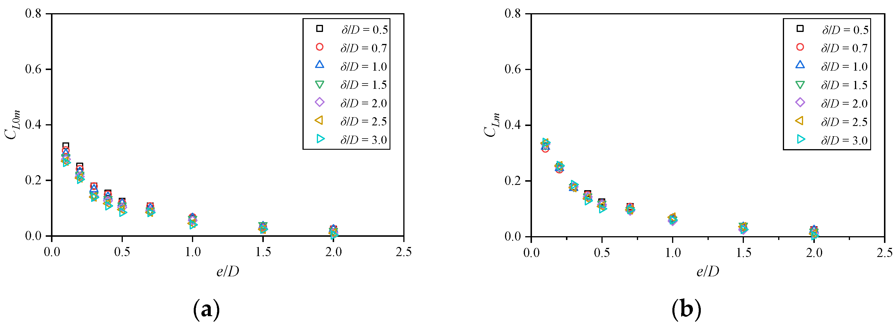
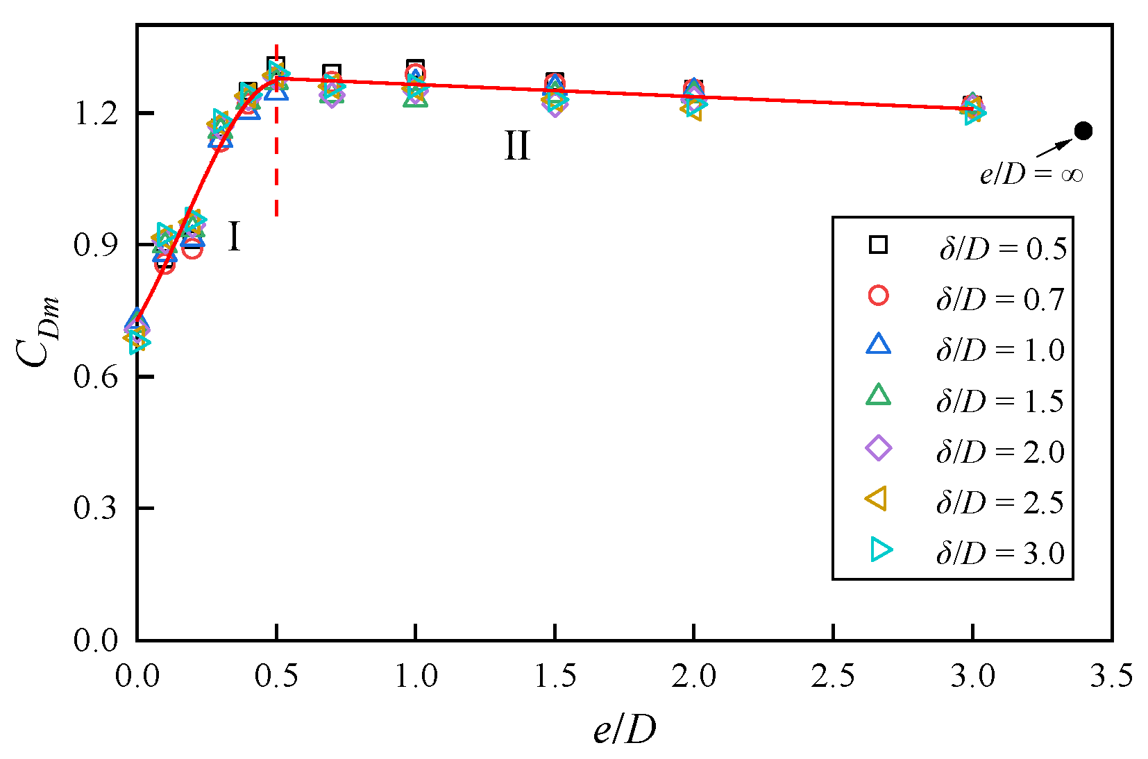
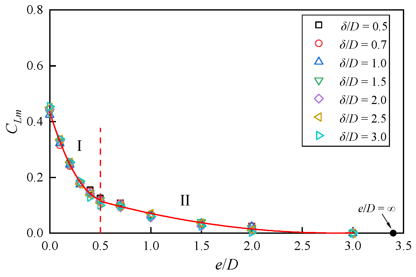
Normalizing the forces with the free stream velocity u₀, the average drag force coefficient C_Dm increases with the increase in e/D for e/D ≤ 0.5 and remains constant for e/D > 0.5. The average lift force coefficient C_Lm gradually decreases with the increase in e/D and approaches zero when the e/D > 1.5. Both C_Dm and C_Lm decrease with the increase in the δ/D. Normalizing the forces with the flow velocity u_a at the center of the pipeline, the influence of the δ/D on C_Dm and C_Lm can be approximately eliminated. Empirical prediction formulas between C_Dm, C_Lm, and e/D are proposed, which can be applied to engineering practices.

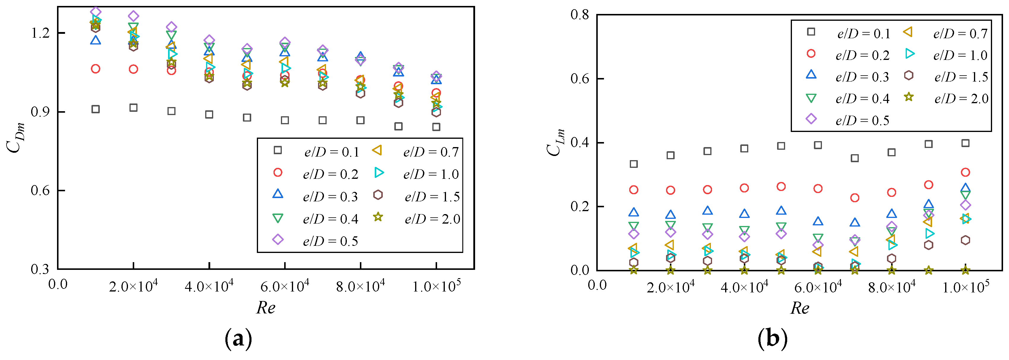
At Re = 10⁴, the vortex shedding is prohibited for e/D < 0.24, where the Strouhal number St is zero. Vortex shedding starts at e/D = 0.24 and St increases with the increase in the e/D for 0.24 < e/D < 0.5. The effect of the wall proximity of vortex shedding is negligible for e/D > 0.5, where St remains approximately unchanged at around 0.2. When Re is in the range of 10⁴ to 10⁵, C_Dm decreases gradually with the increase in Re, whereas C_Lm increases gradually.

References

1. Det Norske Veritas, A.S. On-Bottom Stability Design of Submarine Pipelines,. Recommended Practice, 2021, DNV-RP-F109. Available online: https://www.dnv.com/energy/standards-guidelines/dnv-rp-f109-on-bottom-stability-design-of-submarine-pipelines/ (accessed on 28 April 2025).
2. Det Norske Veritas, A.S. Free Spanning Pipelines. Recommended Practice, 2017, DNV-RP-F105. Available online: https://www.dnv.com/energy/standards-guidelines/dnv-rp-f105-free-spanning-pipelines/ (accessed on 28 April 2025).
3. Liang, D.F.; Cheng, L.; Li, F.J. Numerical modeling of flow and scour below a pipeline in currents: Part II. Scour simulation. Coast. Eng. 2005, 52, 43–62. [Google Scholar] [CrossRef]
4. Kiya, M. Study on the turbulent shear flow past a circular cylinder. Bull. Fac. Eng. Hokkaido Univ. 1968, 50, 1–101. [Google Scholar]
5. Roshko, A.; Steinolfson, A.; Chattoorgoon, V. Flow forces on a cylinder near a wall or near another cylinder. In Proceeding of 2nd US Conference on Wind Engineering Research, Fort Collins, CO, USA, 22–25 June 1975; pp. 4–15. [Google Scholar]
6. Lei, C.; Cheng, L.; Kavanagh, K. Re-examination of the effect of a plane boundary on force and vortex shedding of a circular cylinder. J. Wind Eng. Ind. Aerodyn. 1999, 80, 263–286. [Google Scholar] [CrossRef]
7. Zdravkovich, M.M. Forces on a circular cylinder near a plane wall. Appl. Ocean Res. 1985, 7, 197–201. [Google Scholar] [CrossRef]
8. Teng, Y.; Griffiths, T.; Cheng, L.; Qu, Y.; An, H.; Draper, S.; Gao, Z.; Tang, G.; Lu, L. Effect of steady boundary-layer flow on the hydrodynamic forces on a near-wall cylinder in currents. Ocean Eng. 2024, 313, 119338. [Google Scholar] [CrossRef]
9. Brørs, B. Numerical modeling of flow and scour at pipelines. J. Hydraul. Eng. 1999, 125, 11–23. [Google Scholar] [CrossRef]
10. Kazeminezhad, M.H.; Yeganeh-Bakhtiary, A.; Etemad-Shahidi, A. Numerical investigation of boundary layer effects on vortex shedding frequency and forces acting upon marine pipeline. Appl. Ocean Res. 2010, 32, 460–470. [Google Scholar] [CrossRef]
11. Lei, C.W.; Cheng, L.; Armfield, S.W.; Kavanagh, K. Vortex shedding suppression for flow over a circular cylinder near a plane boundary. Ocean Eng. 2000, 27, 1109–1127. [Google Scholar] [CrossRef]
12. Ong, M.C.; Utnes, T.; Holmedal, L.E.; Myrhaug, D. PE Numerical simulation of flow around a circular cylinder close to a flat seabed at high Reynolds numbers using a k-ε model. Coast. Eng. 2010, 57, 931–947. [Google Scholar] [CrossRef]
13. Menter, F.R. Two-equation eddy-viscosity turbulence models for engineering applications. AIAA J. 1994, 32, 1598–1605. [Google Scholar] [CrossRef]
14. Menter, F.R.; Kuntz, M.; Langtry, R. Ten years of industrial experience with the SST turbulence model. Heat Mass Transfer. 2003, 4, 625–632. [Google Scholar]
15. Oner, A.A.; Kirkgoz, M.S.; Akoz, M.S. Interaction of a current with a circular cylinder near a rigid bed. Ocean Eng. 2008, 35, 1492–1504. [Google Scholar] [CrossRef]
16. Jensen, B.L.; Sumer, B.M.; Jensen, H.R.; Fredsøe, J. Flow around and forces on a pipeline near a scoured bed in steady current. J. Offshore Mech. Arct. Eng. 1990, 112, 206–213. [Google Scholar] [CrossRef]
17. Tang, G.Q.; Cheng, L.; Lu, L.; Teng, Y.F.; Zhao, M.; An, H.W. Effect of oscillatory boundary layer on hydrodynamic forces on pipelines. Coast. Eng. 2018, 140, 114–123. [Google Scholar] [CrossRef]
18. Sumer, B.M.; Fredsøe, J. Hydrodynamics Around Cylindrical Structures; World Scientific Publisher: Singapore, 2006. [Google Scholar]
Figure 1. Schematic of the computational domain.
Water 17 01382 g001
Figure 2. Schematic of pressure and shear stress on pipelines.
Water 17 01382 g002
Figure 3. Mesh diagram: (a) computational grids for the numerical model, and (b) local magnification of grids around the pipeline.
Water 17 01382 g003
Figure 4. Time step convergence verification results: (a) drag coefficient (CD), and (b) lift coefficient (CL).
Water 17 01382 g004
Figure 5. Comparison of average horizontal velocity results: (a) e/D = 0.2, and (b) e/D = 0.3. (The circles represent the experimental data of Oner et al. [15], the red solid lines represent the present numerical results and the dotted lines represent the position for measuring flow velocity).
Water 17 01382 g005
Figure 6. Comparison of average drag/lift coefficients, and root mean square of lift coefficient: (a) average value of the drag force coefficient; (b) average value of the drag force coefficient; and (c) root mean square (RMS) of the lift force coefficient [10,16,17].
Water 17 01382 g006
Figure 7. The relationship between the average drag coefficient and gap ratio for different boundary layer thicknesses: (a) dimensionless treatment using the free stream velocity u0, and (b) dimensionless treatment using the flow velocity ua at the center of the pipeline.
Water 17 01382 g007
Figure 8. The relationship between the average lift coefficient and gap ratio under different boundary layer thicknesses: (a) dimensionless treatment using the free stream velocity u0, and (b) dimensionless treatment using the flow velocity ua at the center of the pipeline.
Water 17 01382 g008
Figure 9. The relationship between the root mean square lift coefficient and gap ratio for different boundary layer thicknesses.
Water 17 01382 g009
Figure 10. The relationship between the Strouhal number and gap ratio for different boundary layer thicknesses: (a) 0.1≤ e/D ≤ 2.0, and (b) 0.2 ≤ e/D ≤ 0.3.
Water 17 01382 g010
Figure 11. The relationship between the average drag coefficient and gap ratio for different boundary layer thicknesses.
Water 17 01382 g011
Figure 12. The relationship between the average lift coefficient and gap ratio for different boundary layer thicknesses.
Water 17 01382 g012
Figure 13. The relationship between the average drag and lift coefficients with Reynolds number for different gap ratios: (a) average value of the drag force coefficient, and (b) average value of the lift force coefficient.
Water 17 01382 g013
Figure 14. The relationship between the Strouhal number and Reynolds number for different gap ratios.
Water 17 01382 g014