
In Situ Hyperspectral Reflectance Sensing for Mixed Water Quality Monitoring: Insights from the RUT Agricultural Irrigation District

 , , , and
Abstract
1. Introduction
2. Related Work
3. Methods
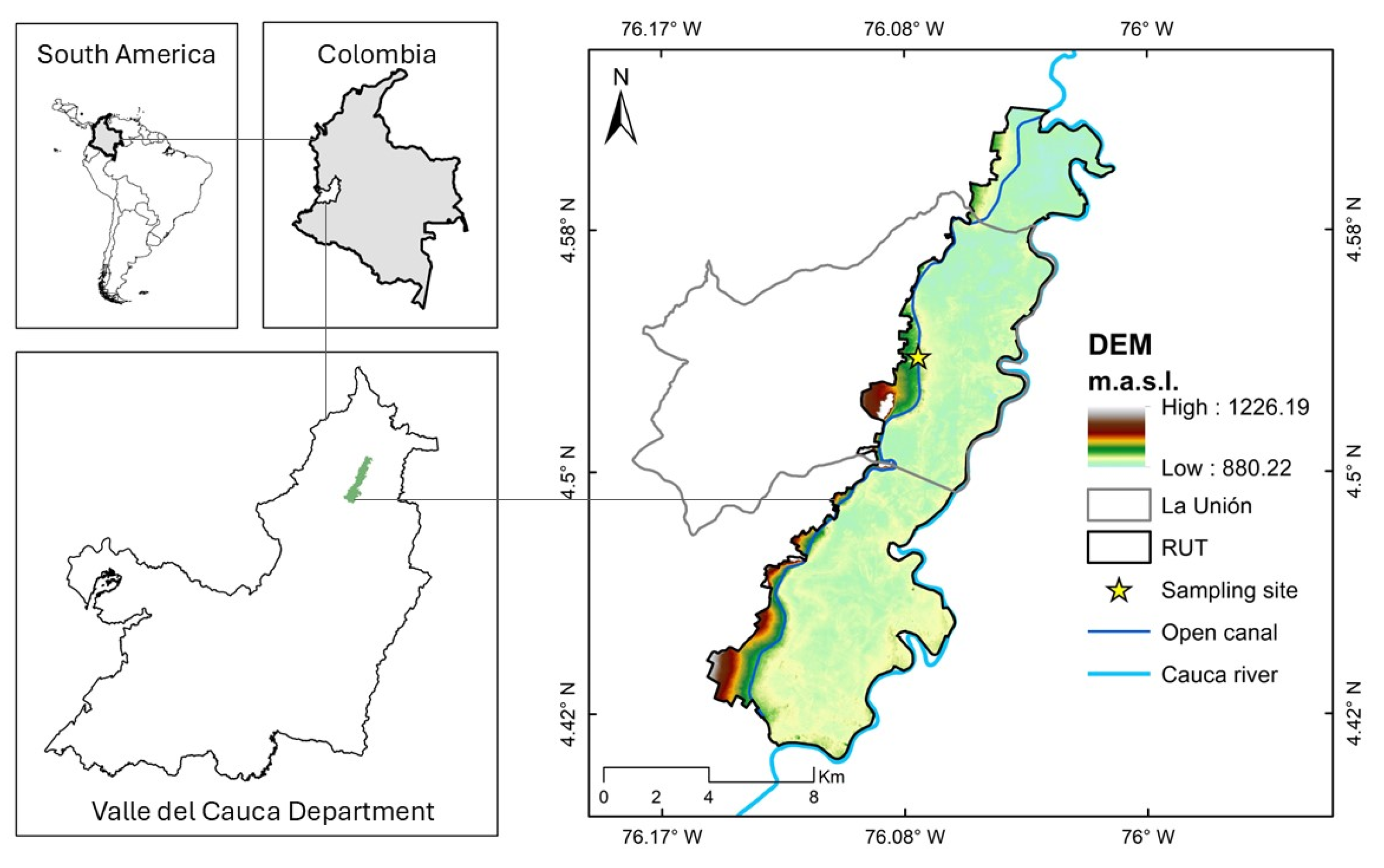
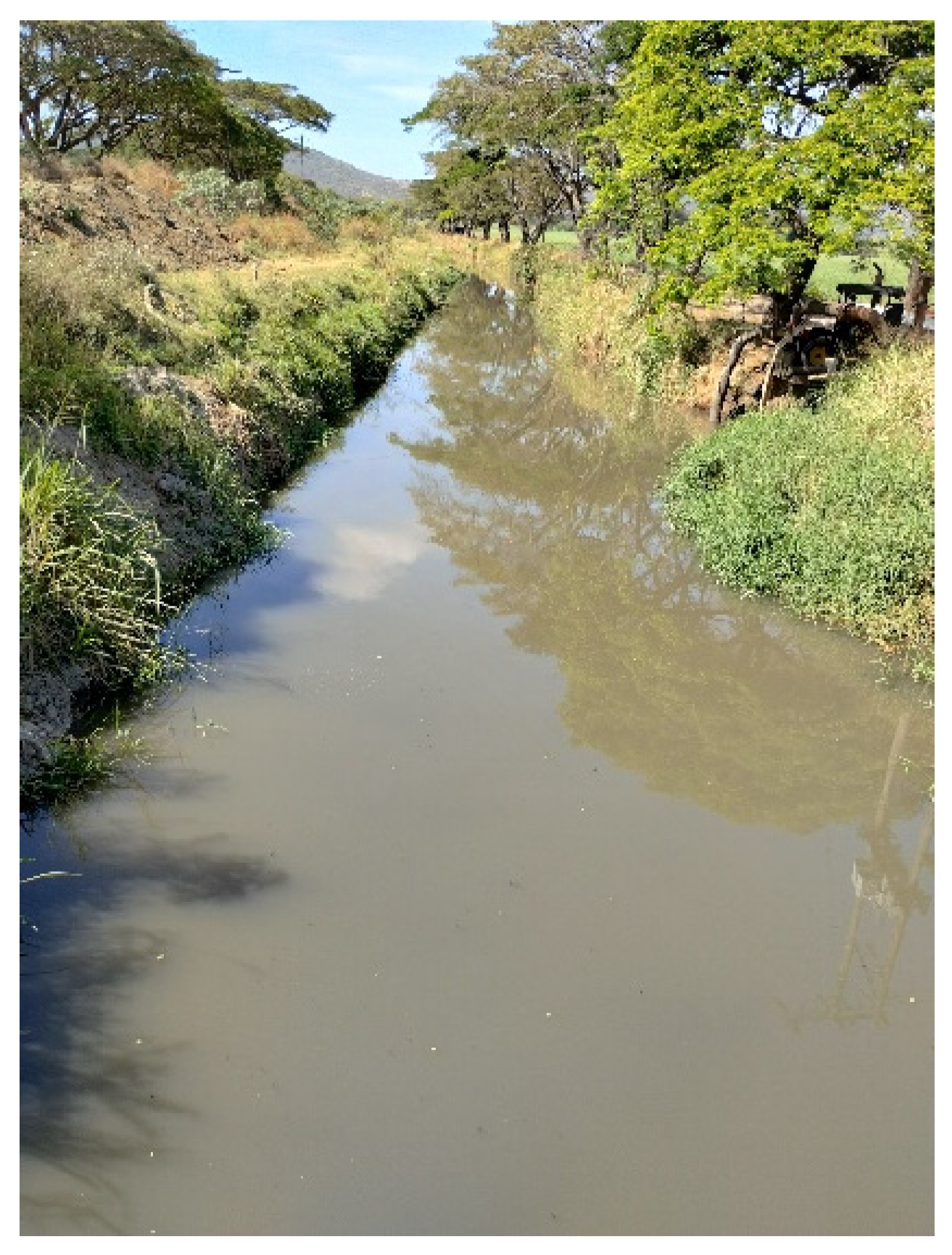
3.1. Study Area
3.2. Water-Quality Parameters Selection
3.3. Data Used
3.3.1. Water Sampling and Laboratory Analysis
3.3.2. Reflectance Measurement and Pre-Treatment
3.4. Statistics
3.4.1. Preprocessing and Pearson Correlations
3.4.2. Non-Linear Analysis
4. Results
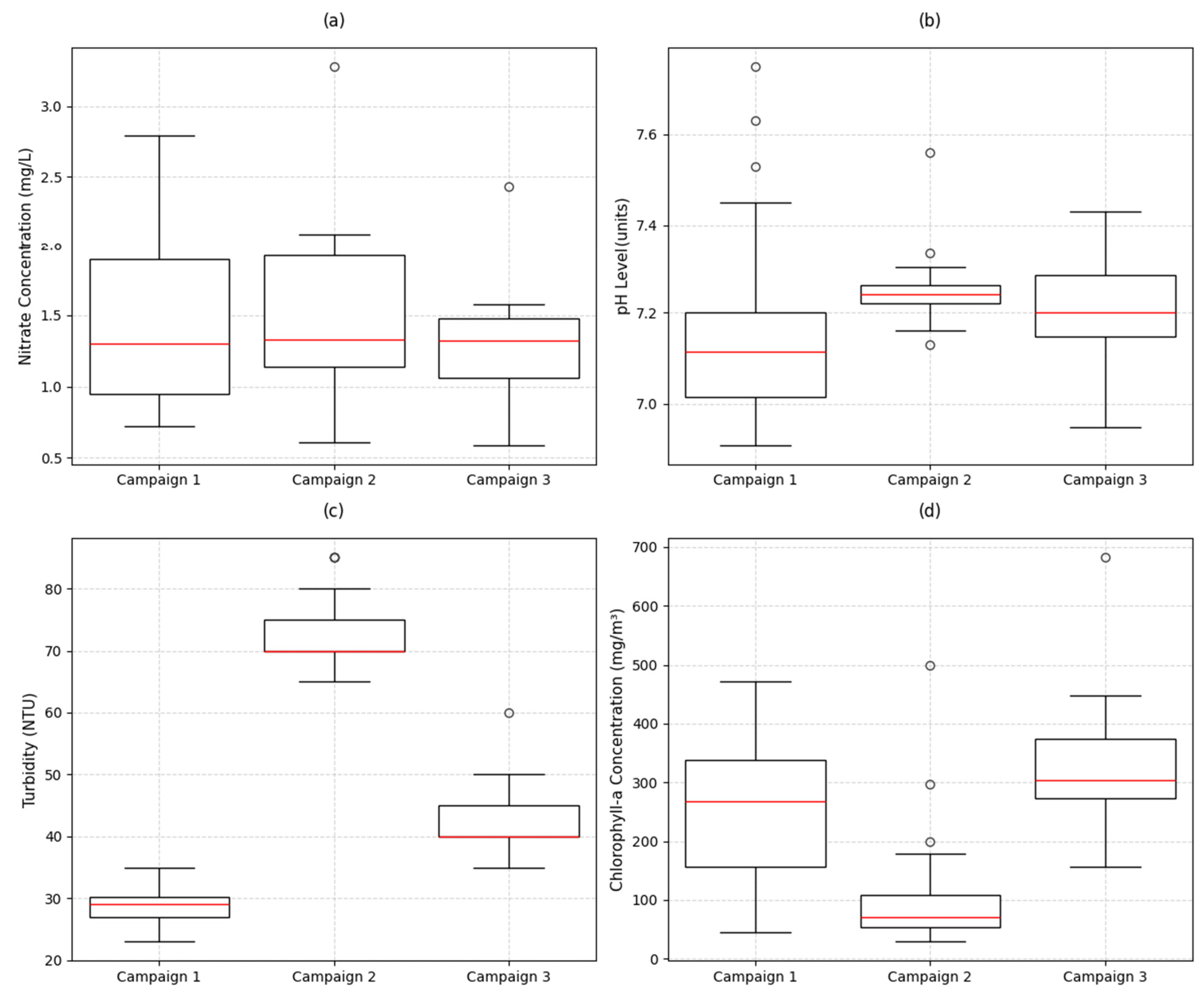
4.1. Water-Quality Parameters Across Campaigns
4.1.1. Campaign 1
4.1.2. Campaign 2
4.1.3. Campaign 3
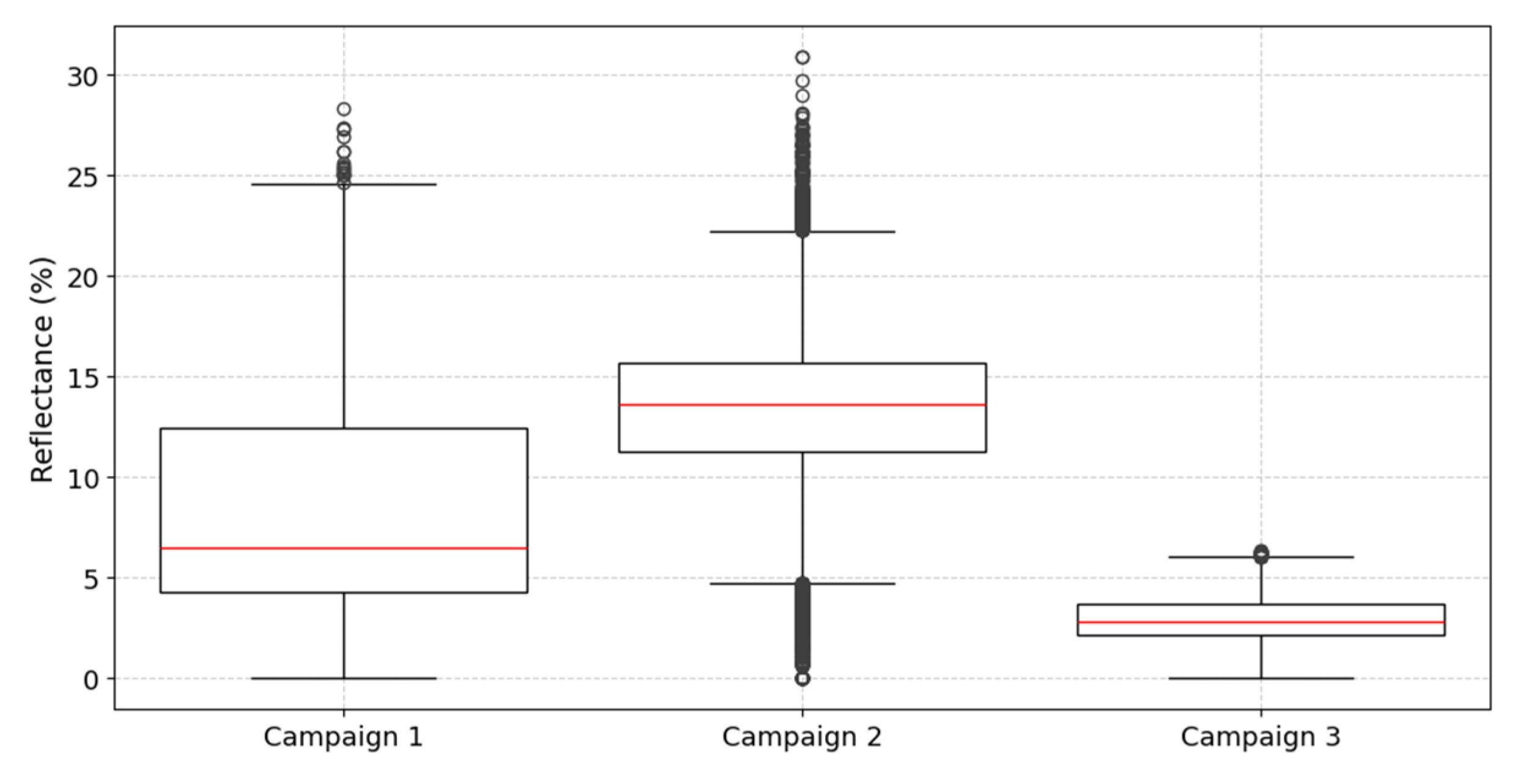
4.1.4. Boxplot of the Hyperspectral Data
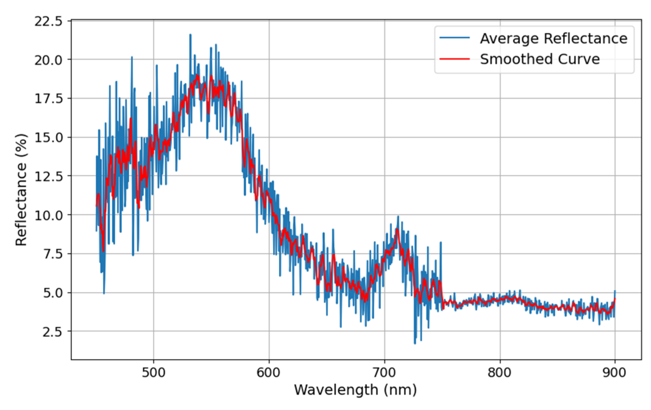
4.2. Average Reflectance Curves
4.2.1. Campaign 1
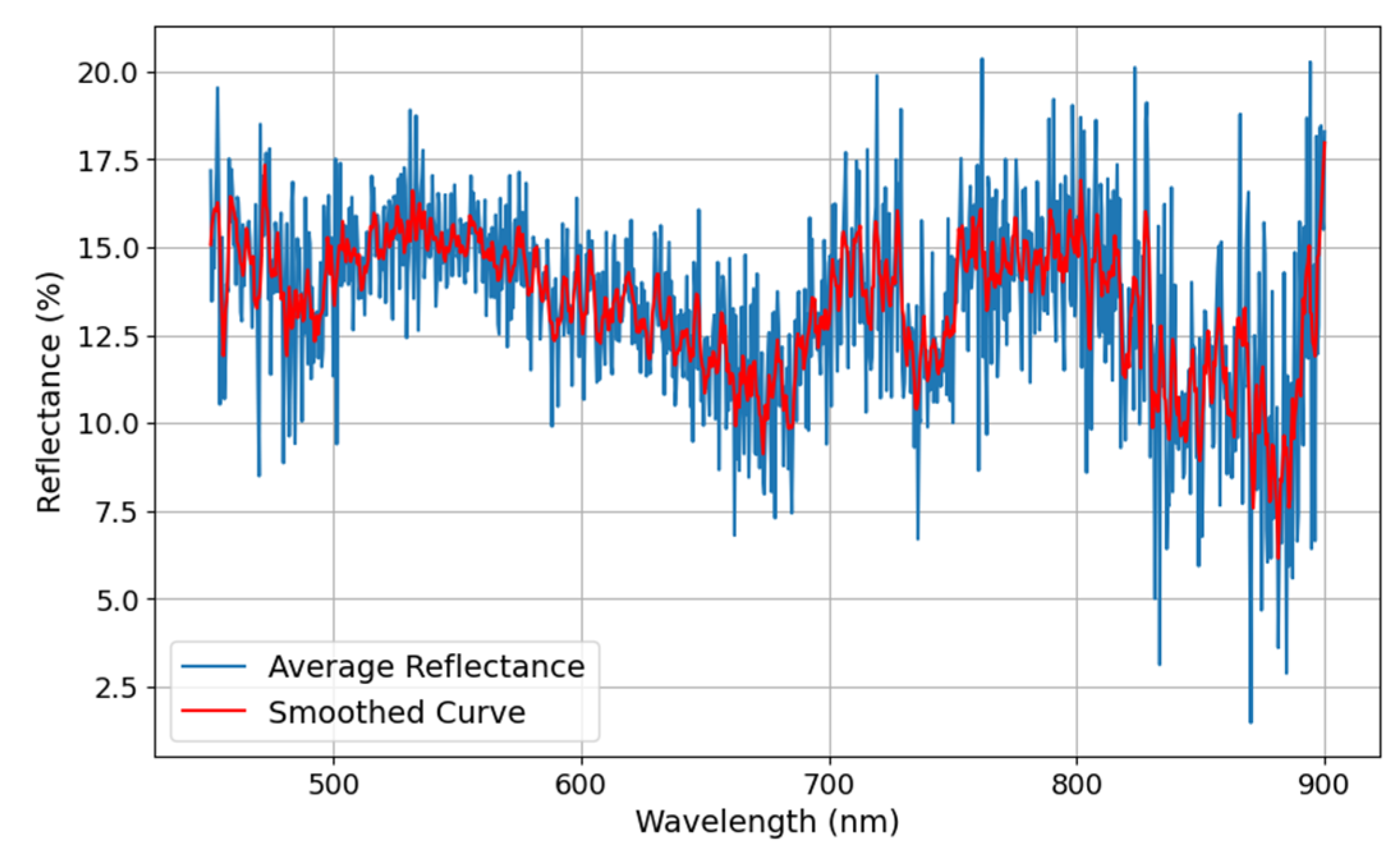
4.2.2. Campaign 2
4.2.3. Campaign 3
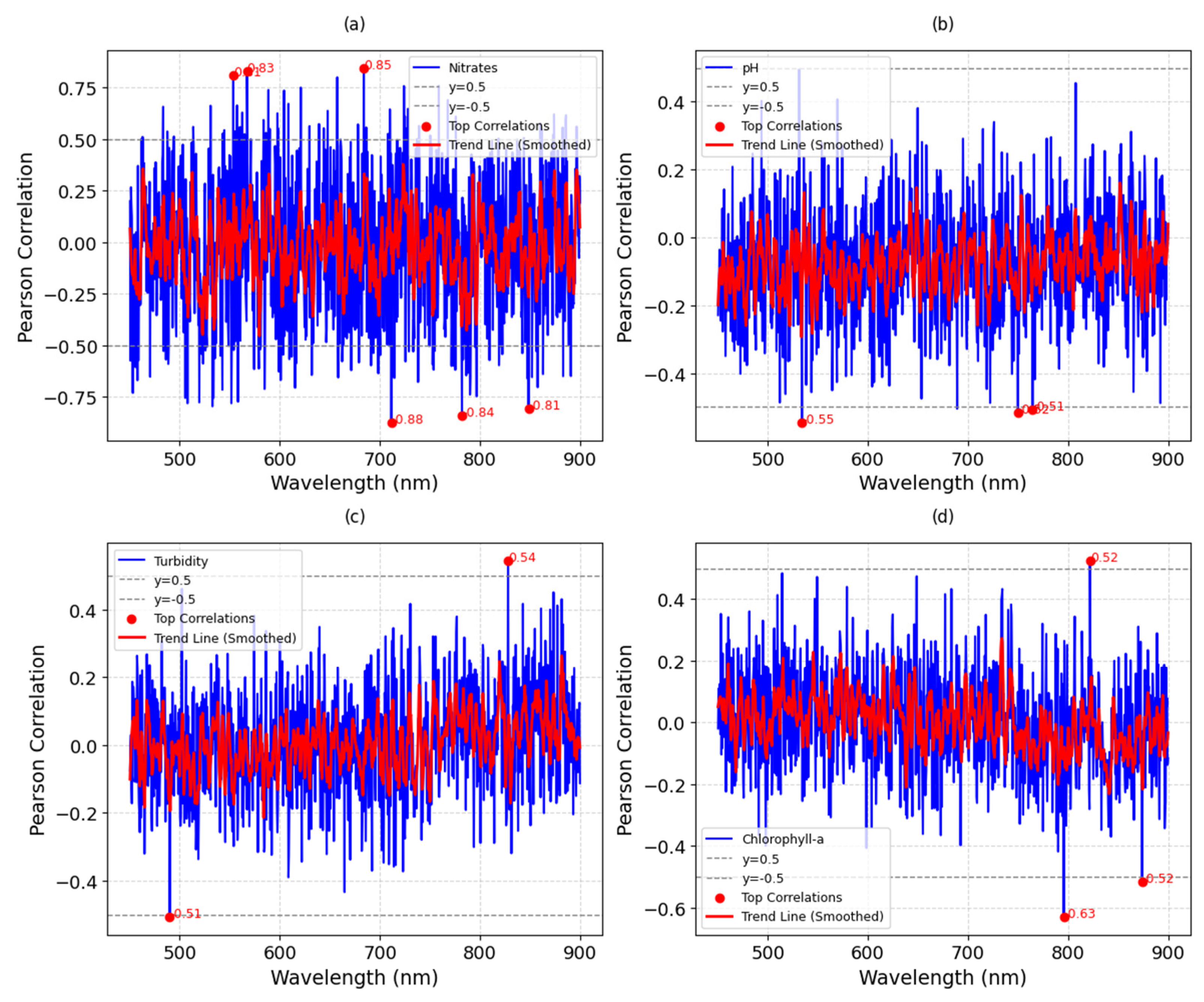
4.3. Active Spectral Regions
4.3.1. Campaign 1
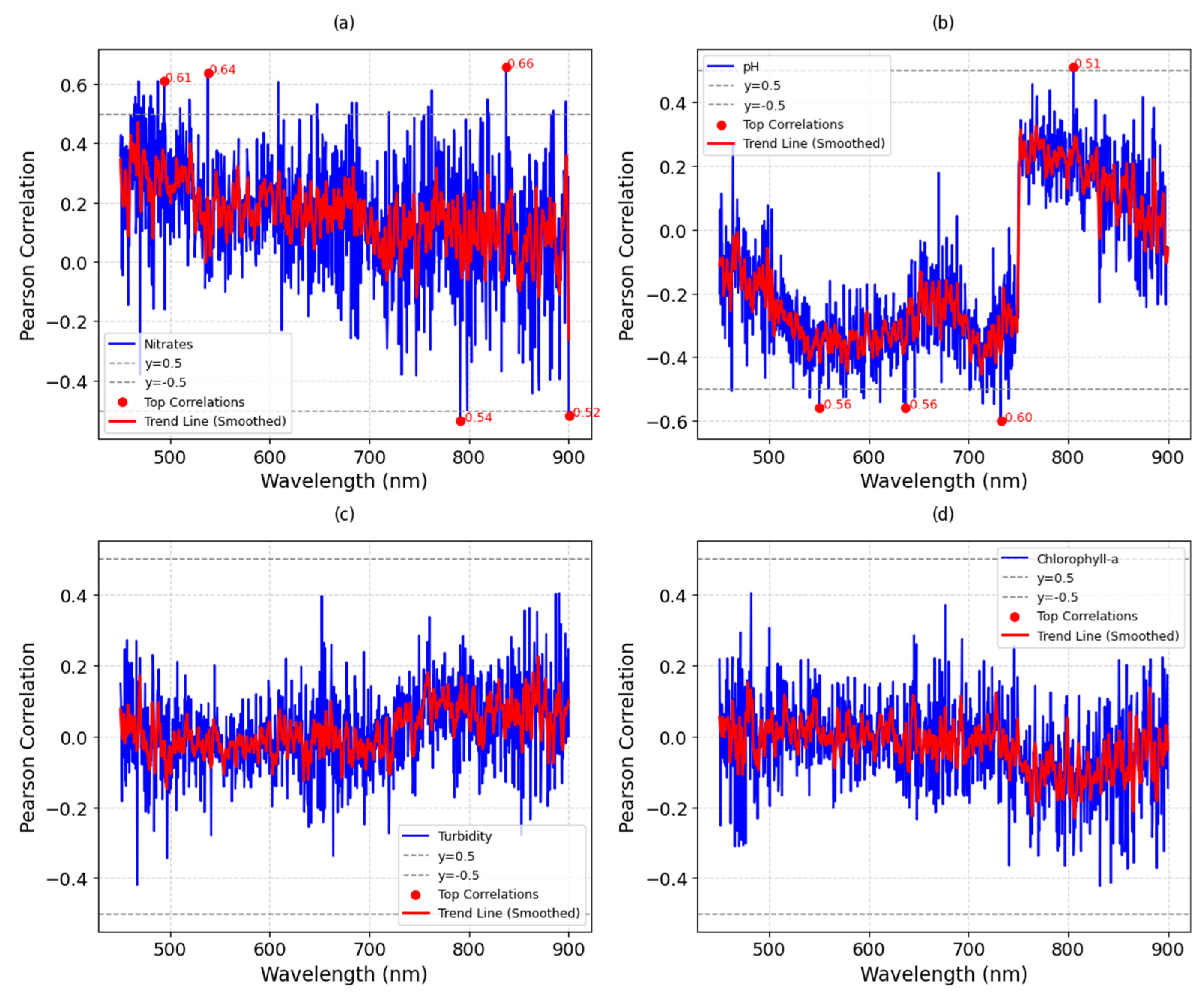
4.3.2. Campaign 2
4.3.3. Campaign 3
4.4. Random Forest Regression
4.4.1. Campaign 1
4.4.2. Campaign 2
4.4.3. Campaign 3
5. Discussion
5.1. Campaign 1
5.2. Campaign 2
5.3. Campaign 3
5.4. Chlorophyll-a
5.5. pH Levels
6. Conclusions
Author Contributions
Funding
Data Availability Statement
Acknowledgments
Conflicts of Interest
References
- Zheng, Y.; Wang, J.; Kondratenko, Y.; Wu, J. Research progress in surface water quality monitoring based on remote sensing technology. Int. J. Remote Sens. 2024, 45, 2337–2373. [Google Scholar] [CrossRef]
- Gholizadeh, M.H.; Melesse, A.M.; Reddi, L. A comprehensive review on water quality parameters estimation using remote sensing techniques. Sensors 2016, 16, 1298. [Google Scholar] [CrossRef]
- Jaramillo, M.F.; Restrepo, I. Wastewater reuse in agriculture: A review about its limitations and benefits. Sustainability 2017, 9, 1734. [Google Scholar] [CrossRef]
- Rahat, S.H.; Steissberg, T.; Chang, W.; Chen, X.; Mandavya, G.; Tracy, J.; Wasti, A.; Atreya, G.; Saki, S.; Bhuiyan MA, E.; et al. Remote sensing-enabled machine learning for river water quality modeling under multidimensional uncertainty. Sci. Total Environ. 2023, 898, 165504. [Google Scholar] [CrossRef]
- Helmecke, M.; Fries, E.; Schulte, C. Regulating water reuse for agricultural irrigation: Risks related to organic micro-contaminants. Environ. Sci. Eur. 2020, 32, 4. [Google Scholar] [CrossRef]
- Yang, H.; Kong, J.; Hu, H.; Du, Y.; Gao, M.; Chen, F. A Review of Remote Sensing for Water Quality Retrieval: Progress and Challenges. Remote Sens. 2022, 14, 1770. [Google Scholar] [CrossRef]
- de Oliveira, M.R.R.; Ribeiro, S.G.; Mas, J.F.; dos Santos Teixeira, A. Advances in hyperspectral sensing in agriculture: A review. Rev. Cienc. Agron. 2020, 51, e20207739. [Google Scholar] [CrossRef]
- Rahul, T.S.; Brema, J.; Wessley GJ, J. Evaluation of surface water quality of Ukkadam lake in Coimbatore using UAV and Sentinel-2 multispectral data. Int. J. Environ. Sci. Technol. 2023, 20, 3205–3220. [Google Scholar] [CrossRef]
- Wei, L.; Wang, Z.; Huang, C.; Zhang, Y.; Wang, Z.; Xia, H.; Cao, L. Transparency Estimation of Narrow Rivers by UAV-Borne Hyperspectral Remote Sensing Imagery. IEEE Access 2020, 8, 168137–168153. [Google Scholar] [CrossRef]
- Uudeberg, K.; Aavaste, A.; Kõks, K.L.; Ansper, A.; Uusõue, M.; Kangro, K.; Ansko, I.; Ligi, M.; Toming, K.; Reinart, A. Optical water type guided approach to estimate optical water quality parameters. Remote Sens. 2020, 12, 931. [Google Scholar] [CrossRef]
- Li, L.; Sengpiel, R.E.; Pascual, D.L.; Tedesco, L.P.; Wilson, J.S.; Soyeux, A. Using hyperspectral remote sensing to estimate chlorophyll-a and phycocyanin in a mesotrophic reservoir. Int. J. Remote Sens. 2010, 31, 4147–4162. [Google Scholar] [CrossRef]
- Cui, M.; Sun, Y.; Huang, C.; Li, M. Water Turbidity Retrieval Based on UAV Hyperspectral Remote Sensing. Water 2022, 14, 128. [Google Scholar] [CrossRef]
- Yim, I.; Shin, J.; Lee, H.; Park, S.; Nam, G.; Kang, T.; Cho, K.H.; Cha, Y.K. Deep learning-based retrieval of cyanobacteria pigment in inland water for in-situ and airborne hyperspectral data. Ecol. Indic. 2020, 110, 105879. [Google Scholar] [CrossRef]
- Arabi, B.; Salama, M.S.; Pitarch, J.; Verhoef, W. Integration of in-situ and multi-sensor satellite observations for long-term water quality monitoring in coastal areas. Remote Sens. Environ. 2020, 239, 111632. [Google Scholar] [CrossRef]
- Cao, Q.; Yu, G.; Sun, S.; Dou, Y.; Li, H.; Qiao, Z. Monitoring water quality of the haihe river based on ground-based hyperspectral remote sensing. Water 2022, 14, 22. [Google Scholar] [CrossRef]
- Sun, X.; Zhang, Y.; Shi, K.; Zhang, Y.; Li, N.; Wang, W.; Huang, X.; Qin, B. Monitoring water quality using proximal remote sensing technology. Sci. Total Environ. 2022, 803, 149805. [Google Scholar] [CrossRef]
- Al-Shaibah, B.; Liu, X.; Zhang, J.; Tong, Z.; Zhang, M.; El-Zeiny, A.; Faichia, C.; Hussain, M.; Tayyab, M. Modeling water quality parameters using landsat multispectral images: A case study of erlong lake, northeast China. Remote Sens. 2021, 13, 1603. [Google Scholar] [CrossRef]
- Zhang, J.; Meng, F.; Fu, P.; Jing, T.; Xu, J.; Yang, X. Tracking changes in chlorophyll-a concentration and turbidity in Nansi Lake using Sentinel-2 imagery: A novel machine learning approach. Ecol. Inform. 2024, 81, 102597. [Google Scholar] [CrossRef]
- Parra, L.; Ahmad, A.; Sendra, S.; Lloret, J.; Lorenz, P. Combination of Machine Learning and RGB Sensors to Quantify and Classify Water Turbidity. Chemosensors 2024, 12, 34. [Google Scholar] [CrossRef]
- Liew, S.C.; Choo, C.K.; Lau JW, M.; Chan, J.; Dang, T.C. Monitoring water quality in Singapore reservoirs with hyperspectral remote sensing technology. Water Pract. Technol. 2019, 14, 118–125. [Google Scholar] [CrossRef]
- Pahlevan, N.; Smith, B.; Schalles, J.; Binding, C.; Cao, Z.; Ma, R.; Alikas, K.; Kangro, K.; Gurlin, D.; Hà, N.; et al. Seamless retrievals of chlorophyll-a from Sentinel-2 (MSI) and Sentinel-3 (OLCI) in inland and coastal waters: A machine-learning approach. Remote Sens. Environ. 2020, 240, 111604. [Google Scholar] [CrossRef]
- Lu, Q.; Si, W.; Wei, L.; Li, Z.; Xia, Z.; Ye, S.; Xia, Y. Retrieval of water quality from uav-borne hyperspectral imagery: A comparative study of machine learning algorithms. Remote Sens. 2021, 13, 3928. [Google Scholar] [CrossRef]
- Qun’ou, J.; Lidan, X.; Siyang, S.; Meilin, W.; Huijie, X. Retrieval model for total nitrogen concentration based on UAV hyper spectral remote sensing data and machine learning algorithms—A case study in the Miyun Reservoir, China. Ecol. Indic. 2021, 124, 107356. [Google Scholar] [CrossRef]
- Lipps, W.; Burton, E.; Baxter, T. (Eds.) Assessment of Aquatic Biology: Chlorophyll-a. In Standard Methods for the Examination of Water and Wastewater, 24th ed.; American Public Health Association: Washington, DC, USA; American Water Works Association: Denver, CO, USA; Water Environmental Federation: Alexandria, VA, USA, 2023; p. 1342. [Google Scholar]
- Reyes-Trujillo, A.; Daza-Torres, M.C.; Galindez-Jamioy, C.A.; Rosero-García, E.E.; Muñoz-Arboleda, F.; Solarte-Rodriguez, E. Estimating canopy nitrogen concentration of sugarcane crop using in situ spectroscopy. Heliyon 2021, 7, e06566. [Google Scholar] [CrossRef]
- Balachandran, S.; Lakshmi, S.; Rajendran, N. Irrigation system using hyperspectral data and machnie learning techniques for smart agriculture. J. Comput. Syst. Sci. 2020, 16, 576–582. [Google Scholar] [CrossRef]
- Kgopa, P.M.; Mashela, P.W.; Manyevere, A. Suitability of treated wastewater with respect to pH, electrical conductivity, selected cations and sodium adsorption ratio for irrigation in a semi-arid region. Water SA 2018, 44, 551–556. [Google Scholar] [CrossRef]
- Zhang, H.; Feng, S.; Wu, D.; Zhao, C.; Liu, X.; Zhou, Y.; Wang, S.; Deng, H.; Zheng, S. Hyperspectral Image Classification on Large-Scale Agricultural Crops: The Heilongjiang Benchmark Dataset, Validation Procedure, and Baseline Results. Remote Sens. 2024, 16, 478. [Google Scholar] [CrossRef]
- El-Hendawy, S.; Al-Suhaibani, N.; Hassan, W.; Tahir, M.; Schmidhalter, U. Hyperspectral reflectance sensing to assess the growth and photosynthetic properties of wheat cultivars exposed to different irrigation rates in an irrigated arid region. PLoS ONE 2017, 12, e0183262. [Google Scholar] [CrossRef]
- Gad, M.; El-Hendawy, S.; Al-Suhaibani, N.; Tahir, M.U.; Mubushar, M.; Elsayed, S. Combining hydrogeochemical characterization and a hyperspectral reflectance tool for assessing quality and suitability of two groundwater resources for irrigation in Egypt. Water 2020, 12, 2169. [Google Scholar] [CrossRef]
- Wu, K.; Ma, F.; Li, Z.; Wei, C.; Gan, F.; Du, C. In-situ rapid monitoring of nitrate in urban water bodies using Fourier transform infrared attenuated total reflectance spectroscopy (FTIR-ATR) coupled with deconvolution algorithm. J. Environ. Manag. 2022, 317, 115452. [Google Scholar] [CrossRef]
- Yan, Y.; Wang, Y.; Yu, C.; Zhang, Z. Multispectral Remote Sensing for Estimating Water Quality Parameters: A Comparative Study of Inversion Methods Using Unmanned Aerial Vehicles (UAVs). Sustainability 2023, 15, 10298. [Google Scholar] [CrossRef]
- Wang, X.; Zhang, F.; Ding, J. Evaluation of water quality based on a machine learning algorithm and water quality index for the Ebinur Lake Watershed, China. Sci. Rep. 2017, 7, 12858. [Google Scholar] [CrossRef]
- Ma, T.; Zhang, D.; Li, X.; Huang, Y.; Zhang, L.; Zhu, Z.; Sun, X.; Lan, Z.; Guo, W. Hyperspectral remote sensing technology for water quality monitoring: Knowledge graph analysis and Frontier trend. Front. Environ. Sci. 2023, 11, 1133325. [Google Scholar] [CrossRef]
- Goyens, C.; Lavigne, H.; Dille, A.; Vervaeren, H. Using Hyperspectral Remote Sensing to Monitor Water Quality in Drinking Water Reservoirs. Remote Sens. 2022, 14, 5607. [Google Scholar] [CrossRef]
- Khadr, M.; Gad, M.; El-Hendawy, S.; Al-Suhaibani, N.; Dewir, Y.H.; Tahir, M.U.; Mubushar, M.; Elsayed, S. The integration of multivariate statistical approaches, hyperspectral reflectance, and data-driven modeling for assessing the quality and suitability of groundwater for irrigation. Water 2021, 13, 35. [Google Scholar] [CrossRef]
- Guo, Y.; Liu, C.; Ye, R.; Duan, Q. Advances on water quality detection by uv-vis spectroscopy. Appl. Sci. 2020, 10, 6874. [Google Scholar] [CrossRef]
- Gan, F.; Wu, K.; Ma, F.; Du, C. In Situ Determination of Nitrate in Water Using Fourier Transform Mid-Infrared Attenuated Total Reflectance Spectroscopy Coupled with Deconvolution Algorithm. Molecules 2020, 25, 5838. [Google Scholar] [CrossRef]
- Alqarawy, A.; El Osta, M.; Masoud, M.; Elsayed, S.; Gad, M. Use of Hyperspectral Reflectance and Water Quality Indices to Assess Groundwater Quality for Drinking in Arid Regions, Saudi Arabia. Water 2022, 14, 2311. [Google Scholar] [CrossRef]
- Saad, M.; Elbeih, S.; Rahman, E.A.; abu Salem, H.S.; Ibrahim, M.; El-Bastamy, E.S. Spectral Indices Based Study to Evaluate and Model Surface Water Quality of Beni Suef Governorate, Egypt. Egypt. J. Chem. 2022, 65, 631–645. [Google Scholar] [CrossRef]
- Zhang, D.; Zhang, L.; Sun, X.; Gao, Y.; Lan, Z.; Wang, Y.; Zhai, H.; Li, J.; Wang, W.; Chen, M.; et al. A New Method for Calculating Water Quality Parameters by Integrating Space–Ground Hyperspectral Data and Spectral-In Situ Assay Data. Remote Sens. 2022, 14, 3652. [Google Scholar] [CrossRef]
- Pinto, A.M.F.; Von Sperling, E.; Moreira, R.M. Chlorophyll-A Determination Via Continuous Measurement of Plankton Fluorescence: Methodology Development. Water Resour. 2001, 35, 3977–3981. [Google Scholar]
- Carvalho, T.M.N.; Neto, I.E.L.; Filho, F.A.S. Uncovering the Influence of Hydrological and Climate Variables in Chlorophyll-A Concentration in Tropical Reservoirs with Machine Learning. Environ. Sci. Pollut. Res. 2022, 29, 74982. [Google Scholar] [CrossRef]
- Wellson, R.; Othman, N.; Matias-Peralta, H.M. The Characterization of Chlorophyll-A and Microalgae Isolation Process of Wastewater Collected at Sembrong Dam. In IOP Conference Series: Materials Science and Engineering; IOP Publishing: Bristol, UK, 2016; Volume 136. [Google Scholar] [CrossRef]
- Taufikurahman, T.; Irene, J.; Melani, L.; Marwani, E.; Purba LD, A.; Susanti, H. Optimizing microalgae cultivation in tofu wastewater for sustainable resource recovery: The impact of salicylic acid on growth and astaxanthin production. Biomass Convers. Biorefinery 2024, 1–10. [Google Scholar] [CrossRef]
- Zhou, X.; Chen, J.; Rakstad, T.E.; Ploughe, M.; Tang, P. Water Chlorophyll Estimation in an Urban Canal System with High-Resolution Remote Sensing Data. IEEE Geosci. Remote Sens. Lett. 2021, 18, 1876–1880. [Google Scholar] [CrossRef]
- Muthuraman, R.M.; Murugappan, A.; Soundharajan, B. Highly effective removal of presence of toxic metal concentrations in the wastewater using microalgae and pre-treatment processing. Appl. Nanosci. 2023, 13, 475–481. [Google Scholar] [CrossRef]
- Wang, C.; Liu, J.; Qiu, C.; Su, X.; Ma, N.; Li, J.; Wang, S.; Qu, S. Identifying the drivers of chlorophyll-a dynamics in a landscape lake recharged by reclaimed water using interpretable machine learning. Sci. Total Environ. 2024, 906, 167483. [Google Scholar] [CrossRef]
- Ahmed, M.; Mumtaz, R.; Anwar, Z.; Shaukat, A.; Arif, O.; Shafait, F. A Multi–Step Approach for Optically Active and Inactive Water Quality Parameter Estimation Using Deep Learning and Remote Sensing. Water 2022, 14, 2112. [Google Scholar] [CrossRef]
- Fu, B.; Li, S.; Lao, Z.; Wei, Y.; Song, K.; Deng, T.; Wang, Y. A novel hierarchical approach to insight to spectral characteristics in surface water of karst wetlands and estimate its non-optically active parameters using field hyperspectral data. Water Res. 2024, 257, 121673. [Google Scholar] [CrossRef]
- Niu, C.; Tan, K.; Jia, X.; Wang, X. Deep learning based regression for optically inactive inland water quality parameter estimation using airborne hyperspectral imagery. Environ. Pollut. 2021, 286, 117534. [Google Scholar] [CrossRef]
- Raheli, B.; Talabbeydokhti, N.; Nourani, V. Uncertainty assessment of optically active and inactive water quality parameters predictions using satellite data, deep and ensemble learnings. J. Hydrol. 2024, 644, 132091. [Google Scholar] [CrossRef]


| Optically active | Chlorophyll-a | [15] (Cao et al., 2022) |
| Turbidity | [13] (Yim et al., 2020) | |
| Optically inactive | pH | [14] (Arabi et al., 2020) |
| Nitrate nitrogen (NO3-N) | [17] (Al-Shaibah et al., 2021) |
| Campaign | Date | Cloudiness (%) | MAT (°C) | WFI |
|---|---|---|---|---|
| 1 | 15 October 2024 | ~20% | 29–30 | Medium |
| 2 | 20 November 2024 | ~30% | 28–29 | Low |
| 3 | 9 December 2024 | ~20% | 30–31 | Medium |
Disclaimer/Publisher’s Note: The statements, opinions and data contained in all publications are solely those of the individual author(s) and contributor(s) and not of MDPI and/or the editor(s). MDPI and/or the editor(s) disclaim responsibility for any injury to people or property resulting from any ideas, methods, instructions or products referred to in the content. |
© 2025 by the authors. Licensee MDPI, Basel, Switzerland. This article is an open access article distributed under the terms and conditions of the Creative Commons Attribution (CC BY) license (https://creativecommons.org/licenses/by/4.0/).
Share and Cite
Benavides-Bolaños, J.A.; Echeverri-Sánchez, A.F.; Reyes-Trujillo, A.; del Mar Carreño-Sánchez, M.; Jaramillo-Llorente, M.F.; Rivera-Caicedo, J.P. In Situ Hyperspectral Reflectance Sensing for Mixed Water Quality Monitoring: Insights from the RUT Agricultural Irrigation District. Water 2025, 17, 1353. https://doi.org/10.3390/w17091353
Benavides-Bolaños JA, Echeverri-Sánchez AF, Reyes-Trujillo A, del Mar Carreño-Sánchez M, Jaramillo-Llorente MF, Rivera-Caicedo JP. In Situ Hyperspectral Reflectance Sensing for Mixed Water Quality Monitoring: Insights from the RUT Agricultural Irrigation District. Water. 2025; 17(9):1353. https://doi.org/10.3390/w17091353
Chicago/Turabian StyleBenavides-Bolaños, Jhony Armando, Andrés Fernando Echeverri-Sánchez, Aldemar Reyes-Trujillo, María del Mar Carreño-Sánchez, María Fernanda Jaramillo-Llorente, and Juan Pablo Rivera-Caicedo. 2025. "In Situ Hyperspectral Reflectance Sensing for Mixed Water Quality Monitoring: Insights from the RUT Agricultural Irrigation District" Water 17, no. 9: 1353. https://doi.org/10.3390/w17091353
APA StyleBenavides-Bolaños, J. A., Echeverri-Sánchez, A. F., Reyes-Trujillo, A., del Mar Carreño-Sánchez, M., Jaramillo-Llorente, M. F., & Rivera-Caicedo, J. P. (2025). In Situ Hyperspectral Reflectance Sensing for Mixed Water Quality Monitoring: Insights from the RUT Agricultural Irrigation District. Water, 17(9), 1353. https://doi.org/10.3390/w17091353