Embankment Project Monitoring Using the Time-Lapse Transient Electromagnetic Method: Numerical Simulation and Field Applications

Abstract

To preserve flood control infrastructure, it is essential to quickly detect and accurately identify concealed leakage hazards within embankment projects. In this paper, we propose a novel embankment monitoring method based on the time-lapse transient electromagnetic method and complemented by a theoretical framework for analyzing time-lapse data through the lens of resistivity change rates. A time-lapse model that scrutinizes dynamic response patterns associated with leakage anomalies is constructed, while the efficacy of this methodology is verified through rigorous field experiments. Our research findings reveal a well-defined negative correlation between the resistivity variation rate and the development stage of anomalies. Our proposed method demonstrates enhanced sensitivity in the detection of dynamic evolutionary patterns in latent seepage defects, particularly in low-resistivity environments. Moreover, it successfully delineates both the spatial expansions and electrical property alterations of anomalies, providing a novel technical approach for latent seepage defect monitoring and risk management in embankments.

1. Introduction

Embankments are integral to flood control infrastructure, and are generally constructed along rivers, lakes, and coastal regions. They are pivotal to safeguarding human life and property [1,2]. Since these structures are often extensive and structurally intricate, they are susceptible to the ravages of time, leading to degradation and the emergence of latent dangers such as cavities or fissures [3,4]. Consequently, the continuous surveillance and precise detection of these hazardous zones have emerged as urgent technical challenges within the domain of water conservation projects [5,6].

Current methodologies employed for the detection of concealed leakage hazards within embankments include geological drilling, manual inspection, and geophysical exploration [6,7,8,9,10]. Although geological drilling is capable of yielding comprehensive and vivid geological data, it is characterized by its extensive labor requirements, significant environmental impact, and substantial expenditure. Meanwhile, manual inspections are constrained by limitations regarding observational scope and efficiency, since they are only effective in identifying superficial threats and are inadequate for pinpointing deep-seated or concealed hazards. In contrast, geophysical exploration, distinguished by its swiftness, non-invasive nature, and cost-effectiveness, has emerged as an effective technique for the detection of embankment-related hazards. It has demonstrated significant utility in the domains of early warning systems and ongoing monitoring [11,12].

In embankment projects, particularly those that involve earth-rock dam structures, the enduring impact of dynamic and hydrostatic pressure within the reservoir region causes the gradual erosion of fine particles within the indigenous loose soil, resulting in the formation of seepage channels or unconsolidated voids [13,14]. These seepages predominantly occur beneath the saturation line within the saturated zone, typically exhibiting lower resistivity than the surrounding medium. Nonetheless, the soil in these seepage areas exhibits minimal resistivity contrast with the surrounding soil, causing the low-resistivity signals to potentially mask other latent electrical anomalies, thereby affecting the effectiveness of electromagnetic detection [15,16]. This phenomenon poses considerable challenges to conventional detection methodologies. In recent years, significant advances have been achieved in embankment monitoring through the utilization of high-density electrical techniques [17,18]. However, in dam engineering monitoring, the use of high-density electrical methods requires the pre-installation of a large number of electrodes, which involves considerable effort. At the same time, as the standardization of the dam progresses, the hardening of the dam surface makes it more difficult to achieve good coupling between the electrodes and the dam body. Furthermore, the detection range of the high-density electrical method is trapezoidal, creating detection blind spots on both sides of the dam shoulder, and its ability to identify deep-seated hazards is relatively limited. These issues somewhat restrict the application of high-density electrical methods in dam monitoring [19,20].

The transient electromagnetic method (TEM) is a detection technology based on the principle of electromagnetic induction that offers advantages such as high detection efficiency, significant detection depth, and independence from topographic relief [21,22]. Existing research has demonstrated the efficacy of time-lapse TEM technology in discerning subtle alterations within subsurface environments through repeated measurements at consistent observation points during varying temporal intervals. This approach demonstrates the notable potential for dynamic monitoring. McLachlan [23] investigated the impact of pertinent noise sources on the quality of time-lapse transient electromagnetic monitoring data. In addition, Zamora-Luria et al. [24,25] presented a steady monitoring instrument centered on transient electromagnetic methods for groundwater level assessment. The findings of these studies validate the potential of time-lapse transient electromagnetic technology in dynamic monitoring and the identification of low-resistivity surroundings. Nevertheless, there remains a research gap regarding the utilization of time-lapse TEM monitoring in embankment projects.

Accordingly, in this study we expound upon existing time-lapse TEM theory, specifically tailoring it for the detection of concealed leakage hazards within embankment projects. The model is validated through a combination of comprehensive three-dimensional numerical simulations and practical field testing. The findings of our study demonstrate the efficacy of this technique in delineating temporal and spatial fluctuations within abnormal zones in low-resistivity environments. Our approach surmounts the constraints associated with conventional detection techniques within low-resistivity terrains, thereby furnishing an indispensable technical foundation for the surveillance and preemptive alert mechanism of potential leakage risks in embankment projects.

2. Methods

2.1. Time-Lapse TEM

The transient electromagnetic method is a geophysical technique that ascertains subsurface electrical properties by emitting brief electromagnetic pulses and subsequently measuring the response from the subterranean medium. It is characterized by its temporal dimension, which pertains to the short time lag between the emission of the pulse and the reception of the response, typically in the millisecond range. Time-lapse TEM is an evolution of conventional TEM that expands upon its temporal dimension. It employs an identical observation system to collect data at distinct temporal intervals within the same geographical location. By doing so, time-lapse TEM enables the monitoring of long-term changes in the subsurface media over days or even months. This approach is particularly suitable for capturing the temporal and spatial dynamics of certain phenomena such as dam leakage, thereby providing insights into their evolution.

Let the forward operator of TEM detection be F, then the detection of each time node can be expressed as:

$$\left(\begin{array}{c}F(m_{\mathrm{T}1})=d_{\mathrm{T}1}\\ F(m_{\mathrm{T}2})=d_{\mathrm{T}2}\\ \cdots \\ F(m_{\mathrm{Tn}})=d_{\mathrm{Tn}}\end{array}\right)$$

(1)

where Tn represents different observation nodes, n signifies observation times, m_Tn denotes the inversion model parameters of different observation time nodes, and d_Tn represents observation data of different time nodes.

When the observed data d_Tn are known, the inversion model parameters of each detection can be obtained by inversion:

$$\left(\begin{array}{c}{m}_{\mathrm{T}1}=F^{-1}(d_{\mathrm{T}1})\\ m_{\mathrm{T}2}=F^{-1}(d_{\mathrm{T}2})\\ \cdots \\ m_{\mathrm{Tn}}=F^{-1}(d_{\mathrm{Tn}})\end{array}\right)$$

(2)

where F⁻¹ is the inversion operator.

The inversion model parameters m_Tn of the dam contain comprehensive geological information such as structure, lithology, and water content. Assuming that there is no hidden seepage hazard in the dam at the first time node T1, and that a seepage hazard develops at time node T2, then:

$$m_{\mathrm{T}1}=m_{\mathrm{T}1 \mathrm{structure}}+m_{\mathrm{T}1 \mathrm{lithology} }+m_{\mathrm{T}1 \mathrm{water}}$$

(3)

$$m_{\mathrm{T}2}=m_{\mathrm{T}2 \mathrm{structure}}+m_{\mathrm{T}2 \mathrm{lithology} }+m_{\mathrm{T}2 \mathrm{water}}$$

(4)

At T2, the internal structure of the dam undergoes structural changes caused by latent seepage defects, while the water-bearing capacity is also altered due to the existence of these defects. However, the lithology of the dam body is not affected, thus:

$$m_{\mathrm{T}1 \mathrm{lithology}}=m_{\mathrm{T}2 \mathrm{lithology}}$$

(5)

From Equation (1) to Equation (5), it can be seen that:

$$m_{\Delta (\mathrm{structure}+\mathrm{water})}=F^{-1}(d_{\mathrm{T}2})-F^{-1}(d_{\mathrm{T}1})$$

(6)

where $m_{\mathsf{\Delta }\left(\mathrm{structure}+\mathrm{water}\right)}$ represents the resistivity variation value due to changes in geological structure and water content.

Equation (6) suggests that time-lapse TEM processing effectively mitigates the influence of the intrinsic geological properties of the dam, relegating them to the background field. Consequently, the model parameters are refined to solely encompass the structural attributes of the dam and the variations in water content that emerge as the seepage hazard evolves.

To further eliminate the influence of the resistivity of the original rock and soil layers on the detection results and to highlight the spatiotemporal evolution characteristics of seepage hazard development, a time-lapse processing method based on the inversion of the resistivity change rate is proposed [8]:

$${\overline{m}}_{\Delta \left(\mathrm{structure}+\mathrm{water}\right)}={\displaystyle \frac{F^{-1}(d_{Tn})-F^{-1}(d_{Tn-1})}{F^{-1}(d_{Tn-1})}}\times 100\%$$

(7)

where ${\overline{m}}_{\mathsf{\Delta }\left(\mathrm{structure}+\mathrm{water}\right)}$ represents the rate of resistivity variation due to changes in geological structure and water content.

2.2. Inversion Theory of Time-Lapse TEM

The objective function of the time-lapse TEM inversion can be expressed as [24]:

$$\phi \left(x\right)={‖d-F\left(m\right)‖}^2+\alpha {‖W\left(m-m_{ref}\right)‖}^2$$

(8)

where d is the observed data, m represents model resistivity, α denotes the regularization factor, W signifies the weight matrix, and m_ref is the node data of the previous time.

The iterative solution of the least square method can be expressed as:

$$m_{k+1}=m_{ref}+{\left(J^T{J}^k+\alpha W^{T}W\right)}^{-1}{J}^T\left(d-F\left(m_k\right)+J^k{m}_k-J^k{m}_{ref}\right)$$

(9)

where J represents the Jacobian operator.

The regularization factor is determined by the L-curve method [26].

3. Numerical Experiment

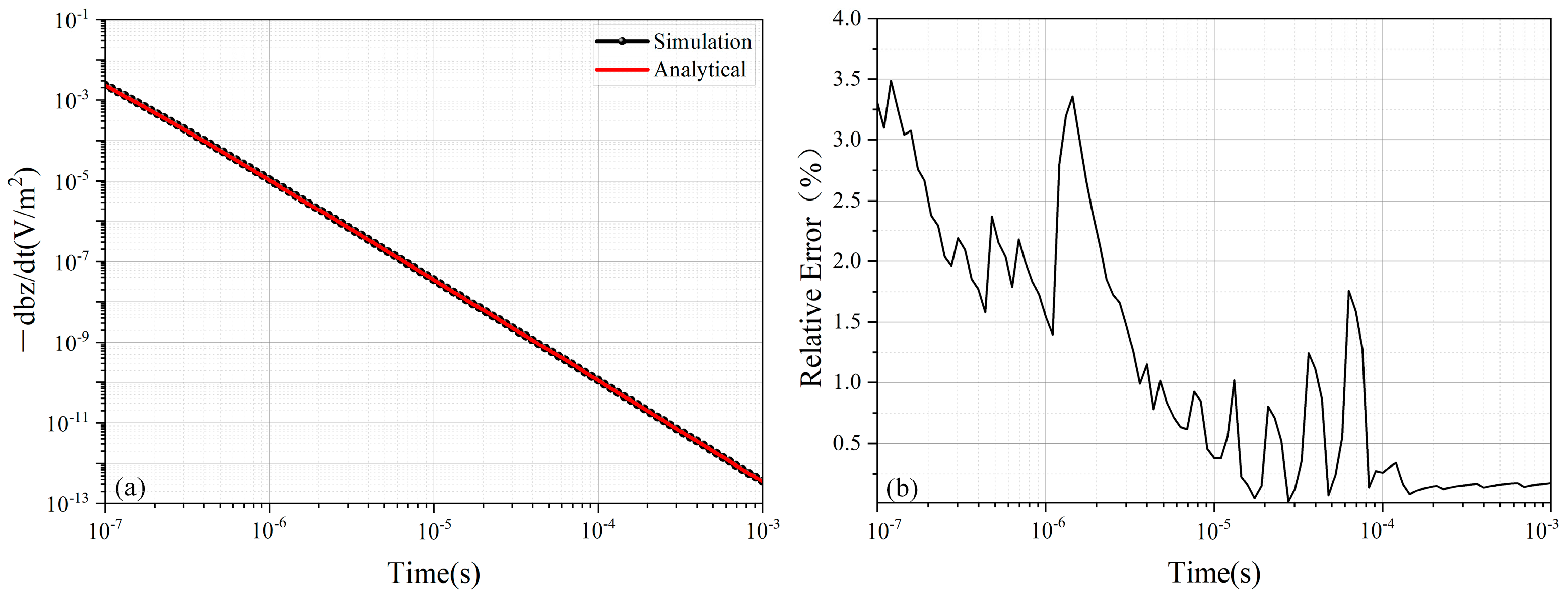
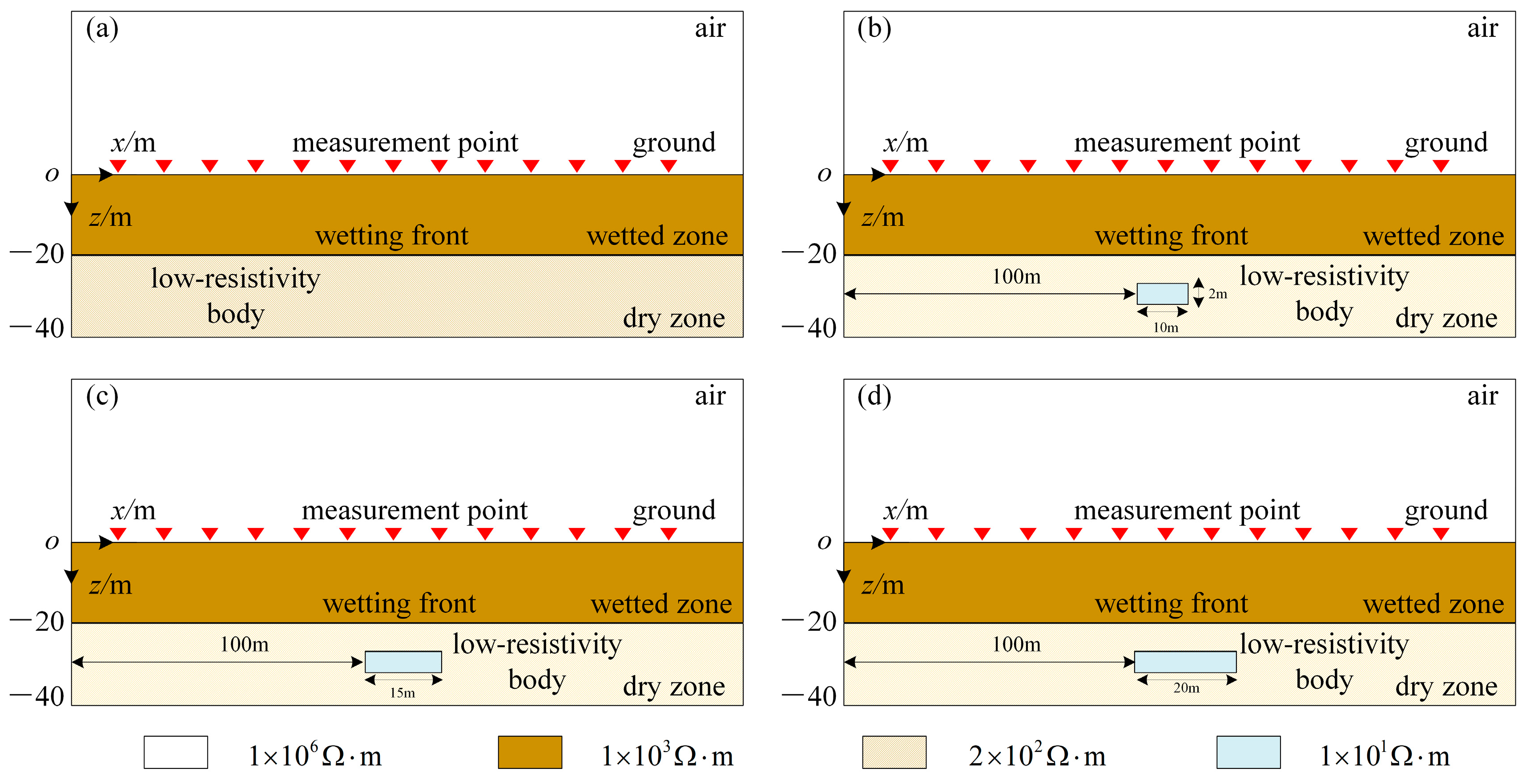
3.1. Model Design and Accuracy Verification

In this study, the finite element algorithm for three-dimensional vector analysis is implemented for numerical simulation. To validate the precision of the algorithm, a standard half-space uniform model is initially established. The dimensions of the model are 400 m × 400 m × 400 m, divided into two distinct layers. The upper layer constitutes an air layer with a thickness of 200 m and a resistivity of 1 × 10⁶ Ω·m, while the lower layer corresponds to the surrounding rock with a thickness of 200 m and a resistivity of 1000 Ω·m. To simulate an infinitely extended space, an eight-layer infinite element boundary with a 20-m thickness surrounding the computational domain is introduced (360 m × 360 m × 360 m) [27]. The excitation source employed in this simulation is a single-turn circular coil with a side length of 1 m, with the receiver positioned at the center of the transmitter coil. A step function is adopted as the transmitting waveform. During the grid partitioning process, the vicinity encompassing the transmission source and receiving point undergoes refinement to ensure the accuracy of the calculations. The induced electromotive force across 101 time channels ranging from 1 × 10⁻⁷ s to 1 × 10⁻³ s is computed and juxtaposed with the analytical solution. Figure 1a presents a comparison of the induced electromotive force curves derived from the numerical solution and the analytical solution, while Figure 1b depicts the corresponding relative error curve. The figures reveal that the two solutions align closely, with the overall error margin never exceeding 4%. This concordance confirms the high accuracy and reliability of the algorithm implemented in this study.

A half-space model is developed to simulate the abnormal evolution of internal leakage within an earth-rock dam. This model aims to analyze the response characteristics of the time-lapse TEM to potential dam hazard areas. The T0 time-lapse model serves as the baseline for this analysis. To simulate the progression of seepage-related hidden dangers within the dam, local low-resistivity anomalies are introduced and incrementally expanded at three subsequent time nodes, designated as T1, T2, and T3. These time nodes correspond to the T1, T2, and T3 models, respectively. The model parameters are defined as follows: the resistivity of air is set to 1 × 10⁶ Ω·m [28], the resistivity of the bedrock in the dam is 1000 Ω·m, the resistivity of the dam material below the saturation line is 200 Ω·m, and the resistivity of the leakage hazard area is 10 Ω·m. We use a rectangular prism to model the anomalous body, which has a rectangular structure with dimensions of a × 10 m × 2 m (length-width-height), where the variable a represents the length of the cuboid in the horizontal direction. To emulate the temporal development of the anomaly, the value of a increases to 10 m, 15 m, and 20 m at time nodes T1, T2, and T3, respectively. The survey line is positioned on the surface of the dam, extending 200 m in length, with an overall dam thickness of 40 m. The thickness of the dam above and below the saturation line is uniformly 20 m on each side. Figure 2 provides a graphical representation of the xoz profile of the model. Figure 3 provides a graphical representation of the xoy profile of the model.

It should be emphasized that, as seepage channels develop within an embankment, the moisture content in the seepage zones increases, whereas that in other parts of the dam may decrease, leading to an increasingly uneven distribution of water. Simultaneously, soil heterogeneity intensifies: the permeability and fabric of the soil surrounding the seepage channels change, thereby enlarging the physical and chemical contrasts in the soil matrix [29,30]. Because the electrical conductivity of an embankment is positively correlated with clay content, moisture content, and void ratio, the growth of seepage channels—by altering these soil properties—significantly influences the spatial distribution of conductivity throughout the structure.

3.2. Analysis of Response Characteristics

Figure 4 depicts the multi-channel profile of the induced electromotive force in the T0~T3 model. Analysis of the cross-sectional data reveals a distinct trend: as the length of the anomalous body gradually increases from 10 m to 20 m, the area of the “bulge” on the induced electromotive force curve expands noticeably and a corresponding enhancement in the bulge amplitude occurs. This observation implies that, as the low-resistivity anomalous body grows in magnitude, there is a progressive rise in the response amplitude of the induced signal and a continuous expansion of the impact zone. Specifically, in the T1 model, the influence range of the anomalous body spans approximately −5 m to 15 m, with the geometric center of the anomalous body located at 105 m along the survey line. In the T2 model, this range widens to −5 m to 25 m, with the geometric center situated at 107.5 m. The range further extends in the T3 model to −5 m to 30 m, with the geometric center at 110 m. These findings demonstrate the relationship between the lateral development of anomalous bodies and the extent of their response zones. Furthermore, as the anomalous bodies develop, the temporal range of their electromagnetic responses progressively elongates, indicating an extension in the time interval. This trend suggests that the anomalous bodies enlarge the response area of the electromagnetic field in the transverse direction. Moreover, they prolong the response duration in the longitudinal direction by intensifying the coupling between the electromagnetic field and the low-resistivity area.

Figure 5 shows the relative values of the T1, T2, and T3 models, which are normalized by the induced electromotive force of the T0 model. To enhance the evaluation of the impact of anomalous bodies on the longitudinal propagation characteristics of induced signals, the T0 model data are utilized as the baseline values to standardize the data of the T1~T3 models. The outcomes reveal that the highest response manifests itself when the relative value of induced electromotive force is consistently at 5.75 × 10⁻⁶ s. Drawing on the smoke ring theory [31], the smoke ring of the transient electromagnetic field at this juncture extends toward the low-resistivity zone. A substantial inductive coupling effect occurs at the anomalous body, culminating in a peak in the response amplitude. This suggests that the positions of maximum response depth across the three models are aligned. After surpassing the threshold of 1.025, the response extents of the three models sequentially expand. The response reach of the T1 model spans from 2.75 × 10⁻⁶ s to 8.32 × 10⁻⁶ s across four time channels, the T2 model broadens to 1.2 × 10⁻⁵ s across five time channels, while the T3 model further extends to 1.74 × 10⁻⁵ s. This observation reveals that as the scale of the abnormal body enlarges, the amplitude of the induced electromotive force escalates in parallel, with a concurrent augmentation in the longitudinal influence range.

3.3. Time-Lapse Monitoring Method

Figure 6 displays the time-lapse transient electromagnetic resistivity variation rate profile of the T1~T3 models, calculated using Equation (7). Figure 6a reveals an obvious negative resistivity change area with a maximum amplitude of approximately −15% within the T1 model embankment. The area spans survey line positions 95–115 m at a depth of about 30 m, which aligns closely with the position of the new low-resistivity anomaly set in the T1 model. Due to the intrinsic volume effect of the transient electromagnetic method [32], the spatial extent of the negative anomaly zone obtained by inversion exceeds the actual dimensions of the model. However, its central location and distribution characteristics exhibit strong consistency with the multi-channel induced electromotive force profile (Figure 4). Additionally, further analysis of the T2 model and T3 model resistivity variation rate profiles (Figure 6b,c) indicates that the centroid of the negative anomaly zone gradually migrates rightward as the seepage fluid expands, centering at 112.5 m (T2 model) and 117.5 m (T3 model) of the survey line. This spatial migration corresponds precisely to the geometric centers of the newly expanded anomaly zones that are incorporated into the model design at each successive time-lapse stage.

A comparative analysis of resistivity variation amplitudes across the T1~T3 time-lapse models shows a gradual decrease in the maximum negative change, from approximately −15% (T1 model) to −12% (T2 model) and then −9% (T3 model). Notably, the model design maintains constant resistivity for the anomalous bodies while simulating their spatial expansion. Thus, although enlarging the anomalous bodies amplifies the overall electromagnetic response, the resistivity variation rate gradually diminishes due to reduced electrical property contrast between the newly expanded and preexisting anomalous regions.

4. Engineering Case

Field testing was conducted at a reservoir in Zhejiang Province, China. The embankment is a clay-core dam with a crest elevation of 183.75 m, base elevation of 163.10 m, maximum height of 25 m, crest length of 126 m, and crest width of 4.5 m. The spillway adopts a side-weir design.

To monitor internal seepage anomalies, time-lapse TEM detection was performed on three occasions: 1 November 2022 (denoted as T0), 23 May 2023 (T1), and 24 August 2023 (T2). To mitigate the shallow blind zone inherent in multi-turn small-loop configurations [33,34], a common-center zero magnetic flux coil with minimal blind zones was employed [35]. TEM measurements were performed with a YSC360A system. The transmitter current was 3 A, the sensor was a zero-flux concentric coil, the repetition (transmit) frequency was 12.5 Hz, the sampling rate was 0.625 MHz, and 1024 stacks were applied [23]. Data were recorded on 120 channels. A 120 m survey line was laid out along the dam crest with a station spacing of 1 m.

Figure 7a presents the resistivity profile at the initial survey time (T0), identifying five low-resistivity anomalies (LRA1-LRA5) as potential seepage zones. Preliminary analysis suggested that LRA1-LRA3 posed higher risks due to possible connectivity, while LRA4 was located downstream near the embankment steps. Based on these findings, grouting reinforcement was applied to LRA1-LRA3, while metal piezometric tubes were installed at 59 m and 91 m along the survey line to monitor pore water pressure.

Figure 7b illustrates the time-lapse resistivity variation profile for T1. After reinforcement, the low-resistivity anomalous bodies in LRA1-LRA3 diminished considerably, with positive resistivity variations indicating effective grouting. We observed low-resistivity anomalies at 59 m (LRA6) and 91 m (LRA7) along the profile that are attributable to the newly installed metallic piezometer casings. These anomalies are spatially clustered and exhibit sharp, localized resistivity contrasts—distinct from the continuous, widespread signatures characteristic of seepage zones—confirming that they originate from the piezometric tubes. Meanwhile, pronounced negative resistivity variations emerged at 80–120 m along the survey line, correlating with minor settlement observed at the dam crest. After careful consideration, a settlement gauge was subsequently installed at 101 m for continuous monitoring of the settlement trend and stability assessment of the dam.

Figure 7c shows the time-lapse resistivity variation profile for T2. By T2 (90 days after T1), the negative anomaly at 80–120 m expanded, reflecting progressive seepage of the dam body in this area. Additionally, a spatially extensive low-resistivity anomaly was observed along the 0–50 m section of the survey line within the shallow depth range of 0–15 m. This anomaly was attributed to the elevated moisture content in the superficial soil layers of the embankment caused by increased rainfall during the local flood season.

5. Discussion

• In genuine embankment environments, seepage processes involve increased pore saturation, elevated ion concentrations, and channel expansion. These events lead to progressive resistivity reduction and a more obvious electrical response. Although our numerical models only expand anomaly dimensions without altering resistivity, the time-lapse transient electromagnetic method effectively captures dynamic expansion trends. Building on this finding, we infer that in real-world dam settings—where resistivity variations coincide with the spatial growth of anomalous zones—the method’s ability to dynamically identify seepage hazards will be even more pronounced. Unexpectedly, we also succeeded in applying the technique to evaluate grouting effectiveness in an engineering case, indicating that time-lapse transient electromagnetic surveys hold promise for grouting monitoring, mine-water hazard assessment, and related applications [36].
• In engineering applications of time-lapse TEM, continuous long-term monitoring remains impractical due to hardware limitations. As a result, repeated surveys replace continuous monitoring. Although some success has been achieved, additional measures are needed to improve the reliability of the monitoring results. For example, the equipment should be calibrated before each data acquisition to ensure consistent instrument performance, the positions of survey stations along the line should be precisely re-established to minimize positional discrepancies and enhance repeatability, and ambient noise should be measured and the data denoised prior to acquisition to eliminate interference caused by environmental noise fluctuations.
• The time-lapse TEM has inherent limitations. In the early stages of seepage-channel development, the resistivity contrast with the surrounding medium is minor, so time-lapse TEM is not sufficiently sensitive to detect nascent seepage paths. Moreover, when several vertically distributed seepage channels occur within the dam body, the method’s vertical resolution is inadequate to distinguish the individual anomalies effectively.

6. Conclusions

In this study, we proposed a time-lapse TEM for embankment monitoring. Furthermore, we analyzed the response characteristics of dynamic changes of abnormal bodies in earth-rock dams through numerical simulations and validated the effectiveness of the method through numerical modeling and field testing. Key conclusions include:

• A resistivity-variation-rate-based time-lapse processing method is derived, effectively eliminating the interference of the dam body soil layer and highlighting the response characteristics of potential seepage-prone zones.
• Results from numerical simulations reveal that the maximum negative resistivity variation consistently localizes at the geometric center of newly expanded anomalies, even when resistivity remains constant and only the spatial scaling of the anomaly body is expanded. This confirms the capability of the time-lapse transient electromagnetic method in resolving spatial expansion trends of subsurface anomalies and sensitively tracking dynamic evolution characteristics of newly expanded anomaly areas.
• Field testing confirms the time-lapse transient electromagnetic method detects latent seepage defects within the embankment and quantifies grouting remediation efficacy. It also delineates the evolution of the seepage zone by analyzing the resistivity changes over different observation periods. This technique provides an effective technical means for embankment project monitoring and risk management.

References

1. Zhang, C.; Wang, G. Water security, and hydroscience and technology in China: Focuses and frontiers. Sci. Sin. Technol. 2015, 45, 1007–1012. [Google Scholar]
2. Feng, Y. Analysis and reflection on characteristics of dikes dangers in middle and lower reaches of Yangtze River in 2020. Yangtze River 2020, 51, 31–33. [Google Scholar]
3. Flores-Berrones, R.; Ramírez-Reynaga, M.; Macari, E. Internal Erosion and Rehabilitation of an Earth-Rock Dam. J. Geotech. Geoenviron. Eng. 2011, 137, 150–160. [Google Scholar] [CrossRef]
4. Yuan, B.; Liang, J.; Huang, X.; Huang, Q.; Zhang, B.; Yang, G.; Wang, Y.; Yuan, J.; Wang, H.; Peng, Y. Eco-efficient recycling of engineering muck for manufacturing low-carbon geopolymers assessed through LCA: Exploring the impact of synthesis conditions on performance. Acta Geotech. 2024. [Google Scholar] [CrossRef]
5. Wang, Y.; Wang, S.; Duan, X.; Gu, Y.; Pang, Q.; Yang, C. Physical modelling of initial seepage failure process. Int. J. Phys. Model Geo. 2015, 15, 220–228. [Google Scholar]
6. Beiranvand, B.; Rajaee, T. Application of artificial intelligence-based single and hybrid models in predicting seepage and pore water pressure of dams: A state-of-the-art review. Adv. Eng. Softw. 2022, 173, 103268. [Google Scholar] [CrossRef]
7. Cen, W.; Du, X.; Li, D.; Yuan, L. Oblique Incidence of Seismic Wave Reflecting Two Components of Design Ground Motion. Shock Vib. 2018, 2018, 412703. [Google Scholar] [CrossRef]
8. Li, F.; Cheng, J.; Chen, S.; Kang, Q.; Li, G.; Liu, D. Fine detection of overburden strata based on time lapse high density resistivity method. Int. J. Min. Sci. Technol. 2019, 4, 1–7. [Google Scholar]
9. Su, H.; Ma, J.; Zhou, R.; Wen, Z. Detect and identify earth rock embankment leakage based on UAV visible and infrared images. Infrared Phys Technol. 2022, 122, 104105. [Google Scholar] [CrossRef]
10. Xiao, P.; Zhao, R.; Li, D.; Zeng, Z.; Qi, S.; Yang, X. As-Built Inventory and Deformation Analysis of a High Rockfill Dam under Construction with Terrestrial Laser Scanning. Sensors 2022, 22, 521. [Google Scholar] [CrossRef]
11. Liu, G.; Hu, J.; Liu, L.; Sun, Q.; Wu, W. Investigating Deformation Mechanism of Earth-Rock Dams with InSaR and Numerical Simulation: Application to Liuduzhai Reservoir Dam, China. Remote Sens. 2023, 15, 4110. [Google Scholar] [CrossRef]
12. Liu, T.; Sun, W.; Kou, H.; Yang, Z.; Meng, Q.; Zheng, Y.; Wang, H.; Yang, X. Experimental Study of Leakage Monitoring of Diaphragm Walls Based on Distributed Optical Fiber Temperature Measurement Technology. Sensors 2019, 19, 2269. [Google Scholar] [CrossRef] [PubMed]
13. Jiang, S.; Fan, Z. Earth-rockfill dam safety classification and risk rate assessment on flood control. J. Hydraul. 2008, 01, 35–40. [Google Scholar]
14. Yuan, B.; Liang, J.; Zhang, B.; Chen, W.; Huang, X.; Huang, Q.; Li, Y.; Peng, Y. Optimized reinforcement of granite residual soil using a cement and alkaline solution: A coupling effect. J. Rock Mech. Geotech. Eng. 2025, 17, 509–523. [Google Scholar] [CrossRef]
15. Shi, X.; Yan, S.; Fu, J.; Chen, M. Time-frequency analysis on influence of low resistive shielding layer in the exploration of transient electromagnetic field. Coal Geol. Explor. 2009, 37, 51–54. [Google Scholar]
16. Li, M.; Liu, S.; Jiang, Z.; Su, B.; Chen, S. Detecting floor geological information bymine DC perspective and 3D inversion. J. China Coal Soc. 2022, 47, 2708–2721. [Google Scholar]
17. Loke, H.; Chambers, J.; Rucker, D.; Kuras, O.; Wilkinson, P. Recent developments in the direct-current geoelectrical imaging method. J. Appl. Geophys. 2013, 95, 135–156. [Google Scholar] [CrossRef]
18. Tao, T.; Han, P.; Ma, H.; Tan, H. 3D Time-lapse resistivity inversion. J. Geophys. 2024, 67, 3973–3988. (In Chinese) [Google Scholar]
19. Oldenborger, G.; Knoll, M.; Routh, P.; LaBrecque, D. Time-lapse ERT monitoring of an injection/withdrawal experiment in a shallow unconfined aquifer. Geophysics 2007, 72, A47–Z71. [Google Scholar] [CrossRef]
20. Bording, T.; Fiandaca, G.; Maurya, P.; Auken, E.; Christiansen, A.; Tuxen, N.; Klint, k.; Larsen, T. Cross-borehole tomography with full-decay spectral time-domain induced polarization for mapping of potential contaminant flow-paths. J. Contam. Hydrol. 2019, 226, 103523. [Google Scholar] [CrossRef]
21. Yue, J.; Zhang, H.; Yang, H.; Li, F. Electrical Prospecting Methods for Advance Detection: Progress, problems, and prospects in Chinese coal mines. IEEE Geosci. Remote Sens. Mag. 2019, 7, 94–106. [Google Scholar] [CrossRef]
22. Lu, T.; Gao, H.; Yang, Y.; Zhou, S. The Transient Electromagnetic Characteristics of Multitarget Unexploded Ordnance (UXO). IEEE Trans. Geosci. Remote Sens. 2024, 62, 2004514. [Google Scholar] [CrossRef]
23. McLachlan, P.; Christiensen, N.; Grombacher, D.; Christiansen, A. Evaluating the impact of correlated noise for time-lapse transient electromagnetic (TEM) monitoring studies. Near Surf. Geophys. 2023, 21, 333–342. [Google Scholar] [CrossRef]
24. Zamora-Luria, J.; McLachlan, P.; Maurya, P.; Liu, L.; Grombacher, D.; Christiansen, A. A feasibility study on time-lapse transient electromagnetics for monitoring groundwater dynamics. Geophysics 2023, 88, E135–E146. [Google Scholar] [CrossRef]
25. Zamora-Luria, J.; McLachlan, P.; Christiansen, A. Long-term monitoring of water table and saltwater intrusion dynamics through time-lapse transient electromagnetic. Near Surf. Geophys. 2024, 22, 636–651. [Google Scholar] [CrossRef]
26. Hansen, P.; O’Leary, C. The Use of the L-Curve in the Regularization of Discrete Ill-Posed Problems. SIAM J. Sci. Comput. 1993, 14, 1487–1503. [Google Scholar] [CrossRef]
27. Zhu, J.; Jiang, Z.; Yin, C.; Qiu, C.; Li, M.; Gao, Z. Finite-element forward modeling of transient EM in mines under metal interference. J. China Coal Soc. 2024, 49, 4578–4589. [Google Scholar]
28. Lu, K.; Yue, J.; Fan, Y.; Li, X.; Zhou, J.; Qi, Y. Three-dimensional transient electromagnetic large-scale forward modeling based on unstructured tetrahedral mesh. J. Geophys. 2025, 68, 327–341. (In Chinese) [Google Scholar]
29. Suski, B.; Revil, A.; Titov, K.; Konosavsky, P.; Voltz, M.; Dagès, C.; Huttel, O. Monitoring of an infiltration experiment using the self-potential method. Water Resour. Res 2006, 42, W08418. [Google Scholar] [CrossRef]
30. Yuan, B.; Chen, W.; Li, Z.; Zhao, J.; Luo, Q.; Chen, W.; Chen, T. Sustainability of the polymer SH reinforced recycled granite residual soil: Properties, physicochemical mechanism, and applications. J. Soils Sediments 2023, 23, 246–262. [Google Scholar] [CrossRef]
31. Xue, G.; LI, X.; Di, Q. The progress of TEM in theory and application. Prog. Geophys. 2007, 04, 1195–1200. [Google Scholar]
32. Cheng, J.; Li, F.; Peng, S.; Sun, X. Research progress and development direction on advanced detection in mine roadway working face using geophysical methods. J. China Coal Soc. 2014, 39, 1742–1750. [Google Scholar]
33. Fan, T.; Zhao, Z.; Wu, H.; Lu, J.; Wang, J. Research on inductance effect removing and curve offset for mine TEM with multi small loops. J. China Coal Soc. 2014, 39, 932–940. [Google Scholar]
34. Yang, H.; Yue, J.; Li, F. The decay characteristics of transient electromagnetic fields stimulated by ramp step current in multi-turn small coil. J. Geophys. 2019, 62, 3615–3628. (In Chinese) [Google Scholar]
35. Hu, X.; Chen, R.; Zhang, P.; Wu, R.; Fu, M.; Zhou, H. Development and experiment of transient electromagnetic common centerzero-flux coil. J. China Coal Soc. 2023, 48, 918–930. [Google Scholar]
36. Guo, Y.; Cui, Y.; Xie, J.; Luo, Y.; Zhang, P.; Liu, H.; Liu, J. Seepage detection in earth-filled dam from self-potential and electrical resistivity tomography. Eng. Geol. 2022, 306, 106750. [Google Scholar] [CrossRef]
Figure 1. Comparison between analytical solution and simulation. (a) Comparison of analytical and simulated induced electromotive force curves, (b) relative error curve.
Water 17 01341 g001
Figure 2. The xoz profile of the four time-lapse models. The left end of the anomaly is located at the 100 m mark along the survey line. (a) is the T0 model, the background model (b) is the T1 model, (c) is the T2 model, (d) is the T3 model.
Water 17 01341 g002
Figure 3. The xoy profile of the four time-lapse models. The left end of the anomaly is located at the 100 m mark along the survey line. (a) is the T0 model, the background model (b) is the T1 model, (c) is the T2 model, (d) is the T3 model.
Water 17 01341 g003
Figure 4. These are the multi-channel profiles of the induced electromotive force corresponding to the four time-lapse models. The horizontal axis represents the measurement point distance, and the vertical axis represents the induced electromotive force. A total of 34 time channels were extracted, ranging from 1 × 10⁻⁷ s to 1 × 10⁻³ s. (a) is the multi-channel profile for the T0 background model, (b) is for the T1 model, (c) is for the T2 model, (d) is for the T3 model. In (b), a slight “bulge” is visible because the emergence of a low-resistivity body produces a locally higher induced electromotive force, this bulge grows progressively larger in panels (c,d) as the anomaly expands.
Water 17 01341 g004
Figure 5. Relative values of the T1, T2, and T3 models normalized by the induced electromotive force of the T0 model. The horizontal axis represents the measurement point distance, and the vertical axis represents the ratio (unitless). (a) T1 model/T0 model, (b) T2 model/T0 model, (c) T3 model/T0 model. In (a), ratios greater than unity reveal a low-resistivity anomaly relative to the background model T0. In (b,c), these ratios increase further, indicating the progressive enlargement and spatial expansion of the low-resistivity body.
Water 17 01341 g005
Figure 6. Time-lapse TEM resistivity variation rate profiles. The black dashed line delineates the seepage zone, and (a), (b), and (c) represent the resistivity variation rate profiles of the T1, T2, and T3 time-lapse models, respectively. (a) (T1 stage): a pronounced negative resistivity variation (deep-blue zone, ~–15%) appears at x ≈ 95–115 m and z ≈ 30 m, coinciding with the location of the newly formed seepage body in the model. (b) (T2 stage): the negative anomaly shifts rightward to x ≈ 110–120 m, its magnitude decreases to ~–12%, and its spatial extent expands slightly compared with T1, indicating continued growth and migration of the seepage body. (c) (T3 stage): the negative anomaly moves further right to x ≈ 115–130 m, its amplitude diminishes to ~–9%, yet it covers the widest area, reflecting an ongoing enlargement of the seepage body and a gradual weakening of the resistivity contrast.
Water 17 01341 g006
Figure 7. Resistivity profile and resistivity variation rate profiles. Seven low-resistivity anomalies (LRA1–LRA7) are marked. (a) Resistivity profile at the initial observation time. (T0), serving as the background, (b) resistivity variation rate profile at T1, (c) resistivity variation rate profile at T2. Based on the dam’s overall apparent resistivity, any value below 100 Ω·m can be regarded as a low-resistivity anomaly. (a) shows the background model, in which five low-resistivity anomalies are identified: LRA1 at x = 15–25 m with resistivity of approximately 75–85 Ω·m; LRA2 at x = 35–45 m with 65–75 Ω·m; LRA3 at x = 50–65 m with 60–75 Ω·m; LRA4 at x = 70–75 m and z = 10–18 m with 20–50 Ω·m; and LRA5 at x = 90–110 m with 80–95 Ω·m. (b) presents the resistivity-variation-rate section for the T1 stage, where two pronounced negative anomalies, LRA6 and LRA7, emerge; meanwhile, the original LRA1–LRA3 zones exhibit positive variation rates (in-creased resistivity), whereas LRA5 shows a negative variation. (c) displays the variation rate section for the T2 stage; relative to (b), new negative resistivity variations appear in the x = 10–15 m and x = 40–80 m intervals, indicating potential seepage risks at these locations.
Water 17 01341 g007aWater 17 01341 g007b
Disclaimer/Publisher’s Note: The statements, opinions and data contained in all publications are solely those of the individual author(s) and contributor(s) and not of MDPI and/or the editor(s). MDPI and/or the editor(s) disclaim responsibility for any injury to people or property resulting from any ideas, methods, instructions or products referred to in the content.