Regionalization-Based Low-Flow Estimation for Ungauged Basins in a Large-Scale Watershed

Abstract

The accurate estimation of low flow is necessary for effective water resource management, especially in regions with limited hydrological data. This study aims to enhance low-flow prediction by developing regional regression models based on climatological variables. Cluster analysis based on Ward’s method and K-means algorithm was applied to delineate hydrologically homogeneous regions within the Nakdong River Basin. Multiple regression models were developed for each cluster to estimate low-flow indicators, Q95 and 7Q. The results demonstrated that regional regression models outperformed the global regression model with log and square-root transformations improving predictive accuracy. Spatial analysis revealed that the key determinants of low-flow estimation may vary across hydrologic conditions, emphasizing the necessity of regionalized approaches for the estimation of low flow due to the limitations of a single global model in heterogeneous watersheds. The proposed methodology is believed to provide a robust framework for hydrological regionalization that can improve the estimation of low flow and support water resource management.

1. Introduction

Low flow refers to the discharge of water in a river during extended dry periods affected by combinations of precipitation input, evapotranspiration losses, and the dynamics of a water storage system within the basin [1,2]. Examining the magnitude and frequency of low flows plays a vital role in the context of water resource management and engineering, which can influence water supply planning, reservoir storage design, irrigation systems, recreational activities, instream flow assessments, and the regulation of river discharge [3]. While there are numerous ways to examine the condition of low flow, the most accurate approach to low-flow analysis starts with collecting observed data to figure out their characteristics. However, the collection of real-time data can be challenging across large scales of watersheds that involve many interactions between separate river sources. The lack of hydrological data on watersheds is troublesome in the analysis of low flows, and the techniques of hydrological regionalization provide a means to estimate hydrological indicators without site-specific calibration and can be applied to infer low-flow characteristics of ungauged basins using information from gauged catchments [4,5].

Regionalization is a widely used technique that can satisfy the lack of hydrological data in areas with limited monitoring resources [6]. This method typically relies on regression analysis between low-flow characteristics and catchment attributes available for ungauged basins [7]. Its practicality benefits water resource planners who should make decisions regarding ungauged watersheds or those with short hydrological records for the reoccurrence period of interest. Extensive research has been focused on regionalization [8,9,10,11,12,13], which can be broadly classified into deterministic and probabilistic approaches. While the deterministic approach uses rainfall–runoff models to generate continuous streamflow time series, the probabilistic approach estimates low flows in ungauged basins by integrating similarity measures and streamflow statistics derived from gauged basins. This method generally consists of two phases: delineating hydrologically homogeneous regions and determining the regression models for low-flow estimation.

The main assumption of delineating hydrologically homogeneous regions is that spatial variability in streamflow characteristics can be explained by watershed attributes [14]. Generally, watersheds with similar climatological conditions tend to exhibit comparable hydrological responses, showing similar patterns in runoff volume and the duration of specific flow periods. Thus, when the study area is extensive or characterized by a highly heterogenous process of low-flow generation, many researchers have proposed a regional regression approach under the appropriate subdivision that can group multiple clusters of homogeneous regions derived from a set of data representing the characteristics of watersheds. The subdivision can help researchers to separately represent the hydrological indicators of interest for each cluster. Cluster analysis has been extensively used for subdividing selected watersheds and is widely recognized as an effective tool in hydrological regionalization, as it facilitates the identification of homogeneous regions. Multivariate statistical methods are employed in the analysis to classify regions, integrating low-flow data and watershed characteristics. Standardization or weighting is typically applied to enhance the discriminative power of the method. Previous studies have adopted this approach [15], using watershed characteristics as the basis for decision making to allocate ungauged sites to the most similar group through spatially discontinuous regional classification.

In the determination of regression models, there are a number of models available including parametric regression, the nearest neighbor method, and the hydrological similarity method [16,17,18]. Among these, parametric regression, commonly known as multiple linear regression, is one of the most widely used approaches. This method establishes a regression equation between optimal parameters and catchment characteristics using data from gauged sites, allowing parameter values to be determined for ungauged basins. In relatively homogeneous regions, a linear function between catchment characteristics and the hydrological indicators of interest can be a reasonable approximation for regional models, and numerous studies have demonstrated the satisfaction of linear regression under hydrologically homogeneous regions [19,20,21]. However, the relationship between catchment attributes and low-flow characteristics is likely to be nonlinear in larger-scale watersheds with more complex hydrological variability. Therefore, combining the delineation of homogeneous regions with regression model development may serve as a robust approach for hydrological regionalization, enhancing the accuracy of low-flow estimates.

The primary objective of this research is to enhance low-flow estimation through a regionalized approach that accounts for spatial heterogeneity in hydrological characteristics. This study was conducted following these steps to achieve the objective: (1) the preparation of climatological variables and low-flow measures, (2) the delineation of hydrologically homogeneous regions using two clustering methods, Ward’s method and the K-means algorithm, (3) the development of a regression model based on the relationship between climatological variables and low-flow measures, and (4) the regionalization of low flow. This research approach is particularly effective for large-scale watersheds, where numerous small to medium-sized streams exist, making the continuous monitoring of all rivers challenging and increasing the likelihood of heterogeneous watershed characteristics. Given these conditions, the methodology is expected to significantly improve low-flow estimation in the selected watershed, providing a strong rationale for conducting this study.

2. Materials and Methods

2.1. Study Area

The Nakdong River Basin, located in the southeastern part of the Korean Peninsula, encompasses the Nakdong River (Figure 1), the second longest river in Korea. Originating in the northeast and flowing southward in the South Sea, the river spans a total length of 510 km, while the basin covers an area of 23,860 km², accounting for 25.9% of the total land area of the Korean Peninsula. As one of the most significant river basins in Korea, it plays a crucial role in water resource management, agriculture, industry, and ecosystem maintenance. The Nakdong River serves as a major water resource, particularly for supplying drinking water, industrial water, and agricultural irrigation to administrative regions located in the midstream and downstream areas. Numerous multipurpose dams and weirs were constructed in the basin to regulate flow and manage water resources. However, the region experiences some of the most severe water conflicts in Korea. For example, during the 2017 drought, 87 agricultural reservoirs within the basin failed to secure sufficient irrigation water, necessitating emergency water supply measures. Similarly, in February 2018, the water storage level of Unmun Dam dropped to 8.2%, prompting the construction of new emergency water supply facilities using river water.

South Korea experiences significant seasonal variations in precipitation, and the increasing frequency of droughts and floods due to climate change has become more pronounced. Despite the presence of numerous hydraulic structures in the basin, the increasing occurrence of low-flow events, exacerbated by concentrated rainfall patterns, poses challenges for upstream dam operations and reservoir regulation, complicating water supply management. Ultimately, the substantial water demand required in large-scale river basins is closely tied to the continuity of water resource supply. Since the inconvenience and damages experienced by the public are directly related to low-flow conditions within the basin, it is essential to first accurately assess low-flow patterns and identify potential issues before implementing responsive measures. Therefore, a proactive analysis of low-flow conditions within the basin is necessary to ensure effective water resource management and mitigation strategies.

2.2. Data Collection for Low-Flow Regionalization

2.2.1. Climatological Variable

The study area was divided into standard watershed units, the smallest subdivision in the water resource unit map used for water resource management. Climatological variables required for low-flow regionalization were then collected based on these units. Sixteen variables that represent the physical characteristics of the watershed and climatic patterns were selected as key factors for assessing their correlation with low-flow conditions (

Table 1. Catchment descriptors used for regression analysis.

Descriptor	Units	Description
Area	km2	Catchment area
LUU	%	Urbanized area
LUC	%	Cropland area
LUF	%	Forested area
WCR	-	Watershed circularity ratio
Smean	%	Mean slope of the catchment
Emax	El.m	Maximum elevation
Emin	El.m	Minimum elevation
Emean	El.m	Mean elevation
SCL	%	Area of silty clay loam
CL	%	Area of clay loam
RCN	-	Runoff curve number
P	mm/year	Mean precipitation
Pd	mm/year	Precipitation in dry period
Pw	mm/year	Precipitation in wet period
RH	-	Relative humidity

). Specifically, the watershed area (Area) represents the spatial scale of hydrological processes within the basin and serves as a critical factor in determining the magnitude of hydrological responses. Land use variables, including urban area (LU_U), agricultural area (LU_C), and forested area (LU_F), influence evapotranspiration and infiltration characteristics, thereby affecting runoff generation. Topographic factors, such as the watershed circularity ratio (WCR) and mean slope of the catchment (S_mean), impact the hydrological response rate and storage capacity. Additionally, maximum elevation (E_max), minimum elevation (E_min), and mean elevation (E_mean) represent the topographic gradient of watershed, playing an important role in determining the flow of precipitation and surface water movement. Soil properties were represented by the proportions of silty clay soil (SCL) and clay soil (CL), both of which are major determinants of soil permeability and water retention capacity [22]. The runoff curve number (RCN), derived from land cover and soil properties, indicates the runoff response of watershed and serves as a key metric for assessing runoff volumes during precipitation events. These watershed characteristics were extracted from the Digital Elevation Model (DEM), slope, and land use maps presented in Figure 2. Climatic factors included annual precipitation (P), dry-period precipitation (P_d), and wet-period precipitation (P_w). The wet period is defined as June to September, while the remaining periods are classified as the dry period. Relative humidity (RH) represents atmospheric moisture content, significantly influencing evapotranspiration and precipitation–runoff processes. Climatic factors were derived from meteorological data collected over the past 30 years (1995–2024) at observation stations within the watershed. These values were expressed as area-weighted averages based on Thiessen polygon interpolation, ensuring a representative spatial distribution of climatic conditions across the basin. All catchment descriptors described above were computed for each selected area and are summarized in Table S1.

2.2.2. Low-Flow Measure

Among 251 streamflow gauges located within the study watershed, 24 gauge stations were selected that satisfied the following three conditions (Figure 3): (i) no presence of upstream dams, (ii) continuous records of daily streamflow available for at least 5 years, and (iii) negligible impact of water withdrawals or diversions during low-flow periods. The streamflow records from 1999 to 2024 were examined, and the data with low reliability or missing data were excluded.

A previous study proposed subdividing nested catchments to treat each segment as an independent watershed, thereby reducing dependency issues and expanding data records [9]. However, the limited number of nested catchments in this study and inconsistencies in consecutive station time series made this approach unsuitable. Additionally, aggregating individual errors could increase overall estimation errors. Therefore, the most trustworthy records of streamflow were solely selected rather than treating all stations as independent to ensure the highest reliability in low-flow estimation.

Based on the observed data from selected gauges, two measures for low flow, the flow exceeded for 95% (Q95) and the minimum flow of 7 consecutive days (7Q), were estimated for each selected area. These two measures were selected as representative of low flow and treated as a foundational data for the development of regionalization and regression model. In particular, Q95 is the indicator derived from the flow duration curve, representing the flow with the time exceedance value of 95%. The indicator, closely related to base flow and commonly used to express long-term sustained levels of flow in a river, reflects extreme conditions of low flow. Similarly, 7Q, which represents the minimum flow of 7 days, serves as a key indicator for assessing extreme low-flow conditions during droughts. Two measures representing low flow for each watershed were annually calculated using data from 24 gauges with proper length of streamflow records. The low-flow measures were computed using all available data across varying weather conditions to observe the possible behavior of low flow.

2.3. Method of Low-Flow Regionalization

2.3.1. Clustering Analysis

Clustering analysis is a technique for partitioning feature vectors into groups that maximize intra-cluster similarity while minimizing inter-cluster similarity. The analysis was extensively applied in low-flow regionalization studies [23,24]. This study employs two widely used clustering methods: Ward’s method, a hierarchical approach, and the K-means algorithm, a partitional approach, both recognized for their effectiveness in hydrological regionalization [25].

Ward’s method, known for its sensitivity to extreme values, enhances cluster precision by minimizing variations among individual vectors. This method estimates cluster distances using analysis of variance, reducing the sum of squared deviations between feature vectors and their cluster centroids [26]. It optimally determines the number of clustering steps in cluster P by minimizing an objective function. In this study, dendrograms were generated for each hierarchical clustering to define the optimal number of groups, and Euclidean distance was employed as the primary metric for distance measurement. The mathematical formulation of this process is as follows:

$$W=\mathrm{m}\mathrm{i}\mathrm{n}\left(\sum _{k=1}^P\sum _{j=1}^M\sum _{i=1}^{N_k}{\left(x_{kij}-{\overline{x}}_{kj}\right)}^2\right)$$

(1)

$${\overline{x}}_{kj}={\displaystyle \frac{1}{N}}\sum _{i=1}^N{x}_{kij}$$

(2)

where W is total within group error sum of squares; $N_k$ denotes the number of gauges in each cluster, M represents the number of attributes; $x_{kij}$ is the jth attribute at the ith gauge in the kth cluster; and ${\overline{x}}_{kj}$ is the average value of the jth attribute in the kth cluster.

The K-means algorithm, a centroid-based partitional clustering method, minimizes an objective function through an iterative relocation process [27]. This algorithm partitions a dataset into clusters while maximizing inter-cluster differences, ensuring an optimal clustering configuration (C). In this study, the Silhouette score S(K) was used to determine the optimal number of clusters (K*). The clustering process is outlined below:

$$S\left(K\right)={\displaystyle \frac{1}{\sum _{k=1}^P{N}_k}}\sum _{k=1}^P\sum _{i=1}^{N_k}{\displaystyle \frac{b\left(i\right)-a\left(i\right)}{max\left(a\left(i\right),b\left(i\right)\right)}}$$

(3)

$$K^{*}=\mathrm{a}\mathrm{r}\mathrm{g}\mathrm{m}\mathrm{a}\mathrm{x}\left\{S\right(K)\mid K\in \left[\mathrm{2,10}\right]\}$$

(4)

$$C=\mathrm{m}\mathrm{i}\mathrm{n}\left(\sum _{k=1}^P\sum _{j=1}^N\sum _{i=1}^{N_k}{\left(x_{kij}-{\mu }_{kj}\right)}^2\right),whereP=K^{*}$$

(5)

where a(i) is the mean intra-cluster distance for data point x_kij, b(i) denotes the mean nearest-cluster distance for data point x_kij, and ${\mu }_{kj}$ is the centroid of the jth attribute in the kth cluster.

2.3.2. Regression Models

This study used a multiple regression model to establish relationships between dependent variables, represented by low-flow measures, and independent variables, which include various climatological factors. Identifying key variables that significantly influence low-flow characteristics allowed for optimizing the regression model to enhance its explanatory power. The regression model was constructed using the Ordinary Least Squares (OLS) method. Low-flow indicators were analyzed using both untransformed values and transformed data to improve model performance. Statistical transformations, including log transformation and root transformation, were applied to address issues related to data distribution. The application of these transformations can improve the robustness of the regression model, ultimately leading to a more reliable framework for low-flow regionalization. The three types of regression model are expressed as follows:

$$Y={\beta }_0+{\beta }_1\times X_i+{\epsilon }_i$$

(6)

$$logY={\beta }_0+{\beta }_1\times X_i+{\epsilon }_i$$

(7)

$$\sqrt{Y}={\beta }_0+{\beta }_1\times X_i+{\epsilon }_i$$

(8)

where Y represents the dependent variable, which corresponds to the low-flow measure in this study. The term β₀ is the intercept, while β₁ is the regression coefficient associated with the independent variable X_i, which denotes a specific climatological factor. The term ε_i accounts for the random error. The OLS method estimates β by minimizing the sum of squared residuals.

Stepwise selection is a representative method for variable selection in statistical modeling, aiming to maximize the explanatory power of a model while eliminating unnecessary variables [28]. The method is classified into forward selection, backward elimination, and stepwise selection, which combines both methods. This study applied the stepwise selection to fit a multiple regression model for each cluster. The method reevaluates the validity of existing variables when adding new ones, ensuring that only the most relevant variables are retained at each step to identify the optimal model. The Akaike Information Criterion (AIC), a widely used metric for evaluating model fit, was employed as the evaluation criterion for deciding whether to add or remove variables. Variable selection was conducted in the direction that minimized the AIC value.

A global regression model, obtained using attributes aggregated from the entire study area, was compared with regional regression models developed separately for each cluster identified through cluster analysis. Precipitation variables were estimated annually to account for low-flow variations due to rainfall patterns, and they were used in the regression analysis corresponding to the low-flow record. Among three precipitation indices, the one having the highest correlation was selected as the representative variable for developing the regression equation. The performance of the regression models was evaluated based on the adjusted coefficient of determination (R_adj²) and mean square error (MSE). Two evaluation metrics are calculated as follows:

$$R_{adj}^2=1-{\displaystyle \frac{n-1}{\left[n-\left(k+1\right)\right]}}\left(1-R^2\right)$$

(9)

$$MSE={\displaystyle \frac{1}{n}}\sum _{i=1}^n{\left(y_i-{\widehat{y}}_i\right)}^2$$

(10)

where n represents the sample size, k denotes the number of independent variables, R² is the sample coefficient of determination, $y_i$ is the observed value, and ${\widehat{y}}_i$ is the simulated value obtained from the regression model. A higher value of R_adj² indicates a better model fit, while a lower MSE signifies reduced prediction error.

3. Results and Discussion

3.1. Delineation of Homogeneous Regions

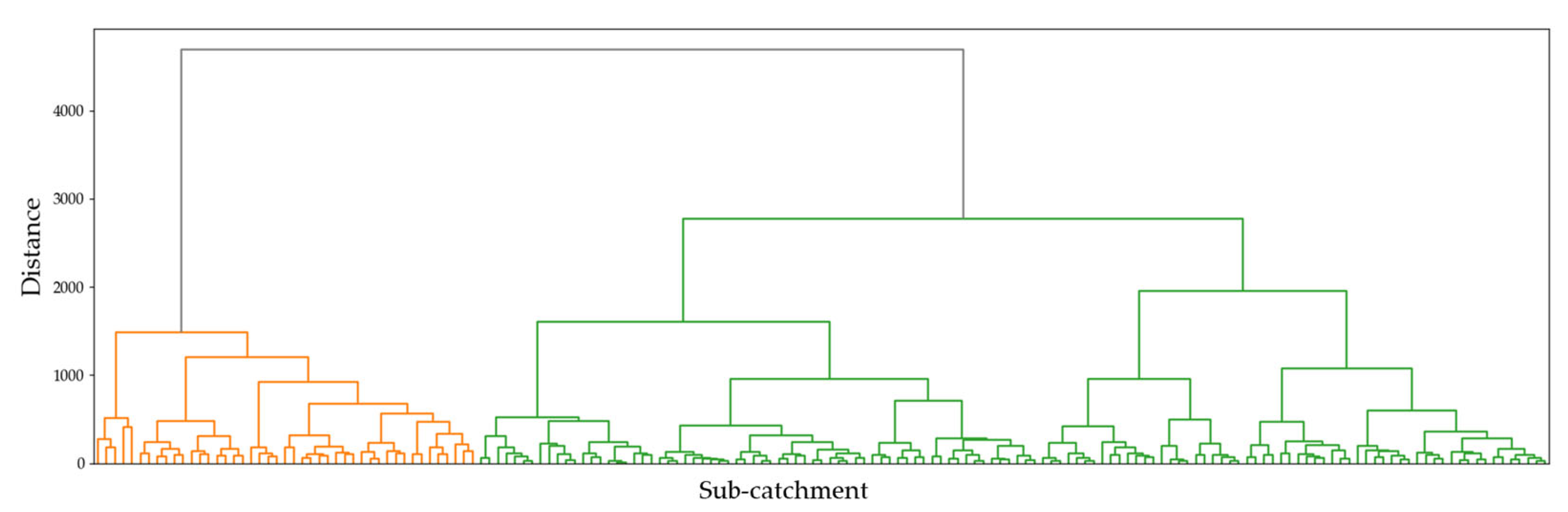
Cluster analysis was performed on a total of 171 sub-catchments, including 24 selected areas to delineate the hydrologically homogeneous regions. The process of determining the optimal number of cluster for two different methods is displayed in Figure 4 and Figure 5. The dendrograms in Figure 4 provide a visual representation of the hierarchical clustering process, where the vertical axis indicates the distance or dissimilarity between clusters. The dendrograms suggest the presence of two primary clusters, as indicated by the significant vertical distance at which the branches merge. The classification into two clusters reflects distinct hydrological or climatological characteristics among the sub-catchments. The selection of the optimal number of clusters was further validated using additional clustering evaluation metrics, ensuring that the chosen clustering structure provides meaningful differentiation in the regionalization of low-flow characteristics. This classification served as the basis for the development of regional regression models tailored to each group.

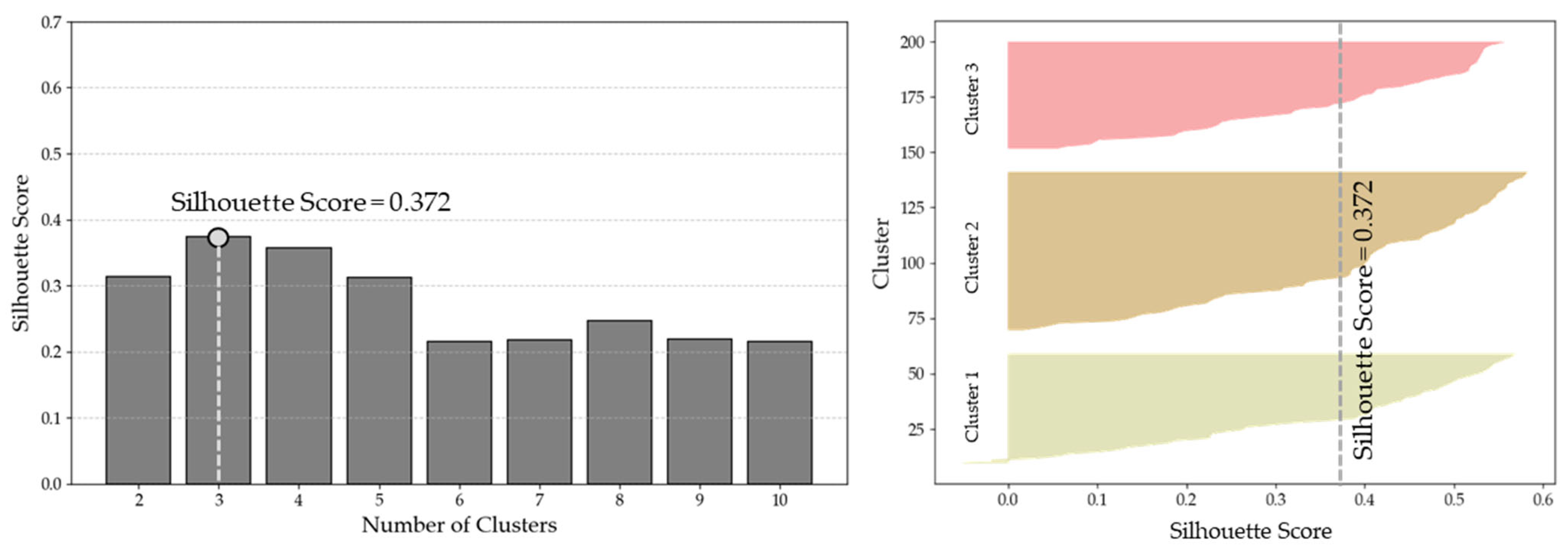
In case of K-means clustering, the optimal number of clusters was determined using the Silhouette score. The left panel of Figure 5 presents the Silhouette scores for different numbers of clusters, indicating that the highest score was observed at three clusters. This suggests that partitioning the dataset into three groups provides the best balance between cohesion and separation. The right panel of Figure 5 displays the Silhouette coefficient distribution for each cluster. The majority of sub-catchments within each cluster exhibit positive silhouette coefficients, confirming that the chosen clustering structure effectively differentiates between groups while maintaining internal consistency. These results support the classification of sub-catchments into three homogeneous regions based on climatological and hydrological characteristics.

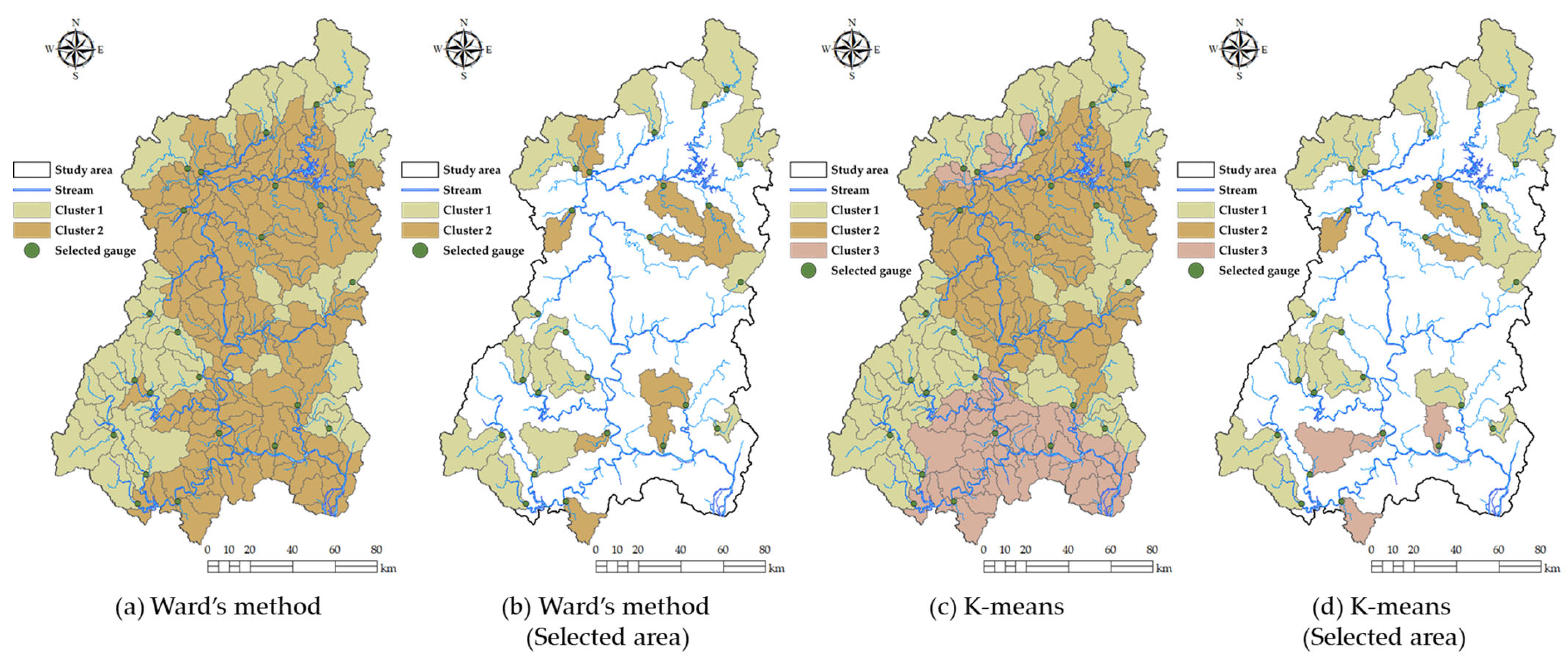
The spatial distribution of homogeneous regions, derived from both Ward’s method and the K-means algorithm, is presented in Figure 6. Panels (a) and (b) illustrate the clustering results for the entire watershed and the selected area (gauged basins) using Ward’s method, while panels (c) and (d) show the corresponding results obtained through K-means clustering. The classification results show the distinct spatial characteristics of sub-catchments based on climatological and hydrological similarities.

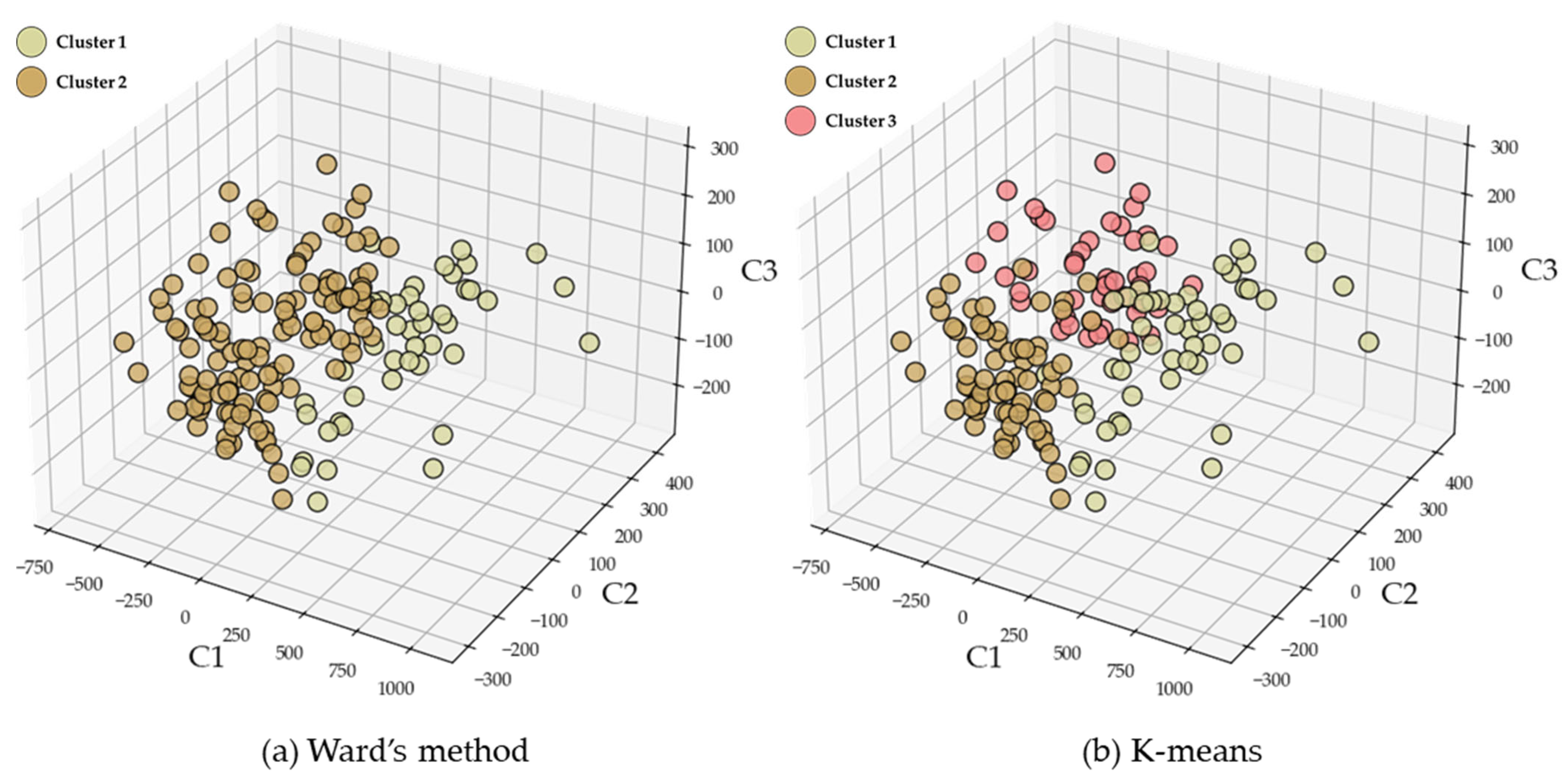
Figure 7 presents a three-dimensional visualization of the classified sub-catchments based on the three components derived from principal component analysis (PCA), which account for the largest variance. Panels (a) and (b) illustrate the clustering results obtained using Ward’s method and the K-means algorithm, respectively. In both methods, a clear separation between clusters is observed, although K-means exhibits a more evenly distributed clustering pattern compared to Ward’s method. The clustering patterns suggest that the identified homogeneous regions effectively capture the underlying climatological and hydrological characteristics of the study area. The PCA-based visualization confirms that the clusters exhibit distinct spatial structures, supporting the reliability of the classification approach. The consistency between the two methods further enhances the robustness of the delineated homogeneous regions.

3.2. Determination of Regression Model

3.2.1. Global Regression Model

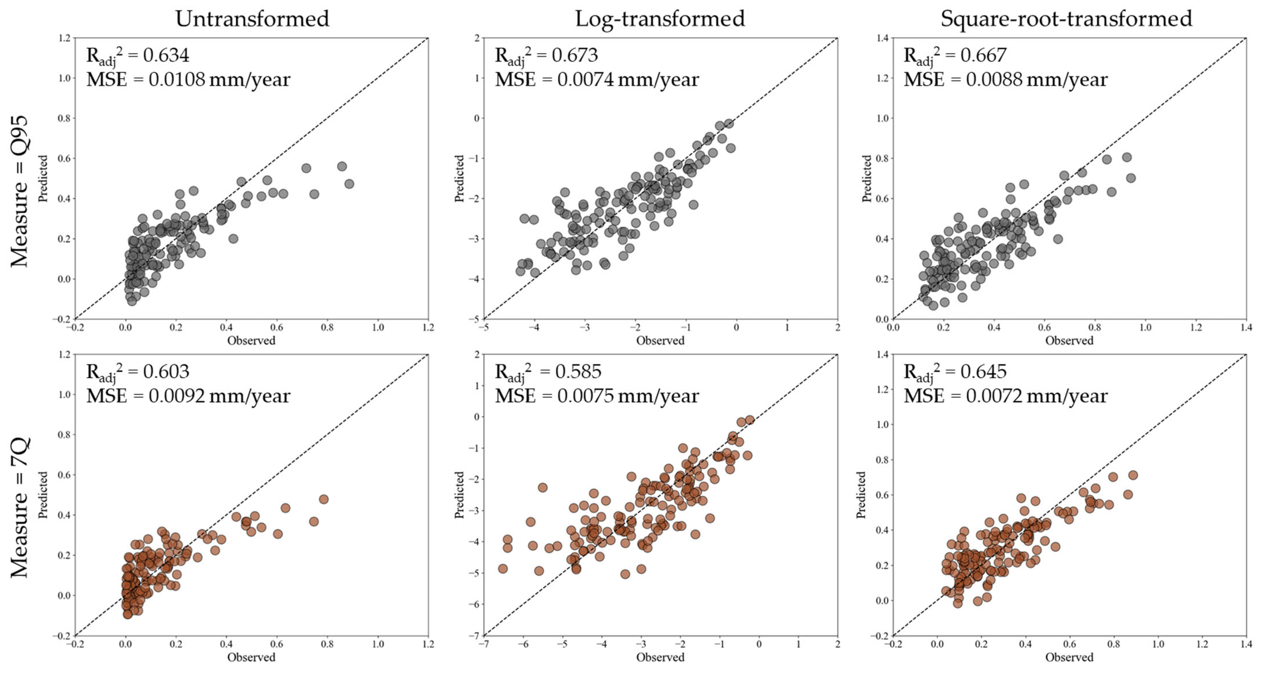
A global regression model was developed to estimate low-flow metrics (Q95 and 7Q) using climatological variables across the study area (Figure 8). For Q95, the log-transformed model exhibited the highest predictive accuracy (R_adj² = 0.673, MSE = 0.0074 mm/year), followed by the square-root-transformed model (R_adj² = 0.667, MSE = 0.0088 mm/year). The untransformed model had the lowest performance (R_adj² = 0.634, MSE = 0.0108 mm/year), suggesting that transformation enhances the performance of the regression model to capture the skewed distribution of Q95 values. For 7Q, the square-root-transformed model performed best (R_adj² = 0.645, MSE = 0.0072 mm/year), slightly outperforming the log-transformed model (R_adj² = 0.585, MSE = 0.0075 mm/year) and the untransformed model (R_adj² = 0.603, MSE = 0.0092 mm/year). These results indicate that log transformation enhances Q95 prediction, whereas square-root transformation better represents 7Q variations by balancing interpretability and predictive accuracy.

The results indicate that data transformation significantly improves regression model performance, particularly for Q95. The log transformation led to a noticeable improvement in R_adj² and a reduction in the MSE, demonstrating that Q95 exhibits a skewed distribution that benefits from logarithmic scaling. For 7Q, the best performance was observed with the square-root transformation, which suggests that this measure follows a moderately skewed distribution rather than a log-normal pattern. The 7-day minimum flow represents a more stable low-flow condition influenced by base-flow contributions, leading to fewer extreme values compared to Q95. Consequently, a square-root transformation appears more suitable for preserving hydrological relationships while enhancing predictive accuracy. Despite the improvements gained through transformation, the global regression model still demonstrates limitations in capturing local variations in low flow. The moderate values of R_adj² suggest that, while the selected climatological and geomorphological predictors explain a portion of low-flow variability, spatial heterogeneity remains a key challenge. This limitation underlines the need for regional regression models, which will be explored in the next section to address spatial variability more effectively.

3.2.2. Regional Regression Model

Based on Ward’s method, regional regression models were developed for Q95 (Figure 9). For Cluster 1, the square-root-transformed model exhibited the highest predictive accuracy (R_adj² = 0.723, MSE = 0.0077 mm/year), followed by the log-transformed model (R_adj² = 0.712, MSE = 0.0084 mm/year). The untransformed model had the lowest performance (R_adj² = 0.634, MSE = 0.0131 mm/year), indicating that transformation effectively improves the ability of the model to capture the distribution of Q95. For Cluster 2, the log-transformed model performed best (R_adj² = 0.655, MSE = 0.0017 mm/year), slightly outperforming the square-root-transformed model (R_adj² = 0.642, MSE = 0.0014 mm/year). The untransformed model (R_adj² = 0.615, MSE = 0.0014 mm/year) showed the lowest predictive accuracy. These results suggest that log and square-root transformations enhance Q95 prediction, with the square-root transformation particularly effective in Cluster 1 and log transformation balancing accuracy and interpretability in Cluster 2.

The regional regression models developed using Ward’s method show clear improvements over the global model, confirming the effectiveness of hydrologically homogeneous clustering in enhancing low-flow predictions. The higher R_adj² values and lower MSEs indicate that regionally calibrated models better capture spatial variations in Q95 compared to a single global model. The superior performance of transformation techniques reinforces the right-skewed nature of Q95. The log transformation showed the best performance in Cluster 1, suggesting that hydrological conditions in this cluster exhibit a stronger skewed distribution. In contrast, Cluster 2 showed similar performance between log and square-root transformations, implying a more stable low-flow regime that benefits from moderate normalization rather than extreme scaling.

The effectiveness of regional regression models in predicting 7Q was evaluated using clusters derived from Ward’s method (Figure 10). For Cluster 1, the log-transformed model exhibited the highest predictive capability (R_adj² = 0.710, MSE = 0.0083 mm/year), followed closely by the square-root-transformed model (R_adj² = 0.695, MSE = 0.0084 mm/year). The untransformed model lagged behind, with the lowest predictive accuracy (R_adj² = 0.668, MSE = 0.0101 mm/year), suggesting that applying transformations enhances model performance by normalizing the skewed distribution of 7Q. In Cluster 2, a similar pattern emerged. The log-transformed model demonstrated the best predictive performance (R_adj² = 0.626, MSE = 0.0010 mm/year), followed by the square-root-transformed model (R_adj² = 0.606, MSE = 0.0009 mm/year). The untransformed model produced the lowest accuracy (R_adj² = 0.493, MSE = 0.0011 mm/year), indicating that a lack of transformation may hinder the performance of the model to capture low-flow variability.

The findings reaffirm that regional regression models developed using Ward’s method improve the predictive accuracy of 7Q estimates. The higher values of R_adj² and reduced MSEs across both clusters demonstrate that spatially calibrated models offer superior performance compared to a single global model. One notable insight from this analysis is the effectiveness of log transformation in enhancing model performance. In Cluster 1, where low-flow characteristics are likely influenced by highly seasonal flow regimes or intermittent base-flow contributions, the log transformation resulted in the best predictive performance. This suggests that 7Q in this cluster exhibits a heavily skewed distribution, where extreme low-flow values require a logarithmic scale for accurate representation. Meanwhile, in Cluster 2, the log and square-root transformations both significantly improved model accuracy, though the log transformation outperformed the others. This result indicates that, while 7Q in this cluster is also right-skewed, it has a more stable base-flow component compared to Cluster 1.

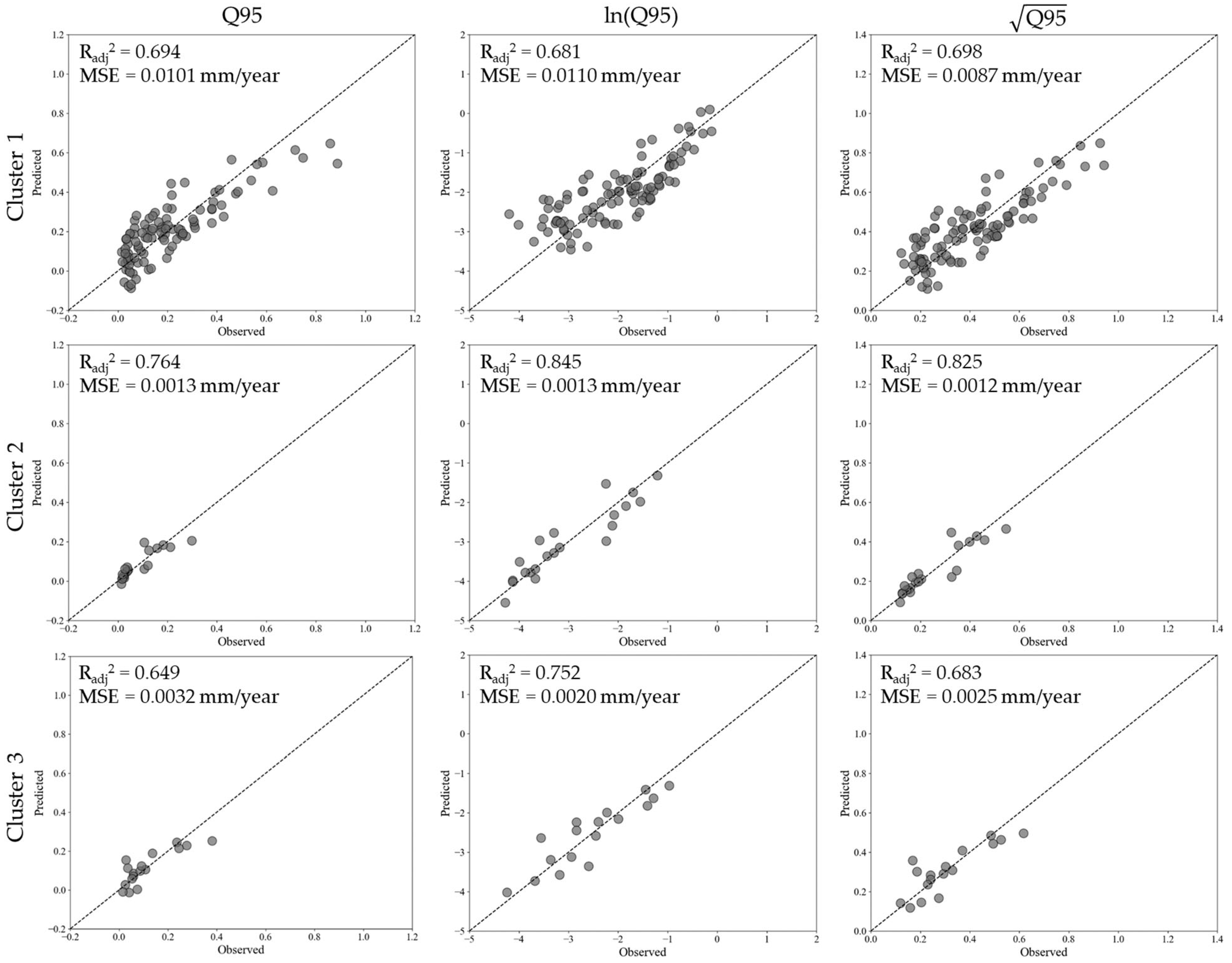
Regional regression models with K-means clustering are constructed for Q95 estimation (Figure 11). In the case of Cluster 1, the square-root-transformed model demonstrated the highest predictive accuracy (R_adj² = 0.698, MSE = 0.0087 mm/year), performing slightly better than the untransformed model (R_adj² = 0.694, MSE = 0.0101 mm/year) and the log-transformed model (R_adj² = 0.681, MSE = 0.0110 mm/year). The relatively minor variations in performance suggest that Q95 in this cluster follows a less skewed distribution, resulting in limited benefits from transformation. For Cluster 2, the log-transformed model achieved the best results (R_adj² = 0.845, MSE = 0.0013 mm/year), surpassing both the square-root-transformed model (R_adj² = 0.825, MSE = 0.0012 mm/year) and the untransformed model (R_adj² = 0.764, MSE = 0.0013 mm/year). In Cluster 3, the log-transformed model again provided the most accurate predictions (R_adj² = 0.752, MSE = 0.0020 mm/year), followed by the square-root-transformed model (R_adj² = 0.683, MSE = 0.0025 mm/year) and the untransformed model (R_adj² = 0.649, MSE = 0.0032 mm/year).

The analysis showed the strong influence of transformation on model accuracy, particularly in Clusters 2 and 3. The log-transformed model consistently provided the best performance. Notably, minimal differences in transformation performance for Cluster 1 suggest that low flows in this region are more stable and require less extreme normalization. The comparable accuracy of the untransformed model implies that Q95 in this cluster may be governed by relatively uniform hydrological processes. On the other hand, the effectiveness of K-means clustering in delineating hydrologically distinct regions is evident in the clear differences in model behavior across clusters. Unlike Ward’s method, which produces hierarchical clusters, K-means allows for greater flexibility in identifying statistically similar sub-catchments, leading to robust regression models.

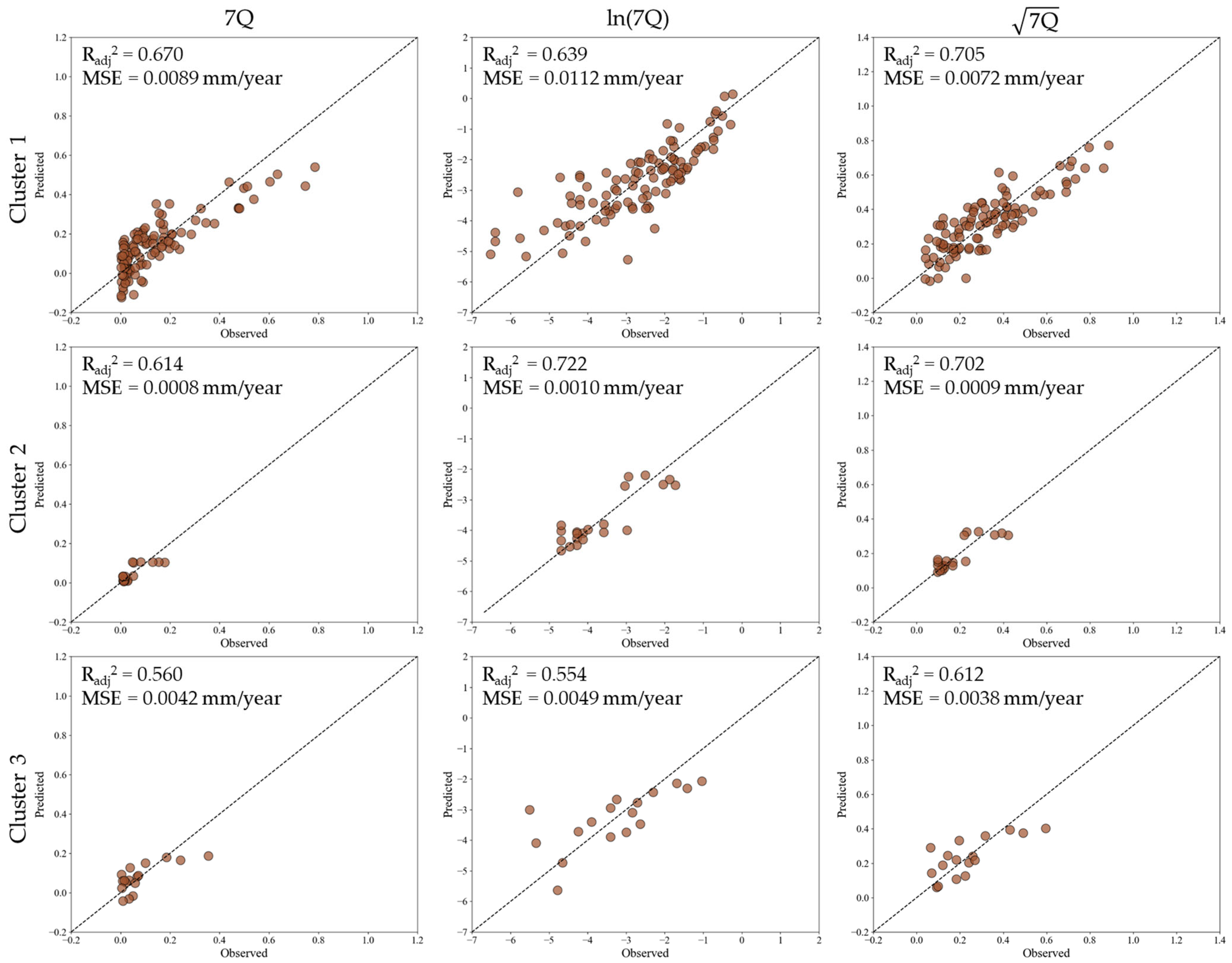
Regional regression models for 7Q under K-mean clustering conditions were also developed to allow for low-flow variability (Figure 12). As a result, in Cluster 1, the square-root-transformed model delivered the best performance (R_adj² = 0.705, MSE = 0.0072 mm/year), slightly outperforming the untransformed model (R_adj² = 0.670, MSE = 0.0089 mm/year) and the log-transformed model (R_adj² = 0.639, MSE = 0.0112 mm/year). The relatively minor differences in transformation effects suggest that 7Q in this cluster follows a moderately skewed distribution, with square-root transformation providing an optimal balance between interpretability and predictive power. For Cluster 2, the log-transformed model achieved the highest accuracy (R_adj² = 0.722, MSE = 0.0010 mm/year), followed closely by the square-root transformation (R_adj² = 0.702, MSE = 0.0009 mm/year). The untransformed model lagged behind (R_adj² = 0.614, MSE = 0.0008 mm/year), demonstrating that transformation substantially enhances predictive accuracy in this region. For Cluster 3, all models performed relatively poorly compared to other clusters, but the square-root transformation provided the highest accuracy (R_adj² = 0.612, MSE = 0.0038 mm/year), surpassing both the untransformed model (R_adj² = 0.560, MSE = 0.0042 mm/year) and the log-transformed model (R_adj² = 0.554, MSE = 0.0049 mm/year). These results indicate that 7Q in this cluster may be influenced by localized hydrological controls that are not fully captured by the regression models.

3.3. Low-Flow Regionalization

Both Q95 and 7Q demonstrated better explanatory power in regression models under K-means clustering, and the regression model of Q95 showed improved accuracy with log transformation, while that of 7Q performed better with square-root transformation. Based on these findings, low-flow regionalization was conducted using these two specific models with the global regression model for each measure as a comparison target.

The analysis of the ln(Q95) model revealed that key factors influencing hydrology varied across clusters. In Cluster 1, precipitation, maximum elevation, runoff curve number, mean slope, and area size were identified as the primary variables, indicating that complex processes including climate, runoff generation, and topographic structure influence low-flow formation. In Cluster 2, precipitation in wet period and mean elevation emerged as the significant variables, highlighting the importance of seasonal precipitation variability and topography. In Cluster 3, precipitation, runoff curve number, and area size were identified as key factors. The analysis of the $\sqrt{7\mathrm{Q}}$ model also revealed distinct regional differences in low-flow formation processes. Cluster 1 exhibited key influencing variables similar to those of Q95. In contrast, Clusters 2 and 3 showed different patterns. In Cluster 2, mean precipitation and mean slope were identified as the primary factors, whereas, in Cluster 3, the mean precipitation and runoff curve number were determined to be the major variables for low-flow estimation.

These model selection results emphasize the significance of regional hydrological characteristics in low-flow estimation. The variation in predictor variables across clusters proves the necessity of regionalization, demonstrating that a single global model fails to adequately capture the variability of climatic and topographic factors. Furthermore, the findings provide strong evidence that regional regression models outperform global models. While global models offer a broad-scale understanding of low-flow characteristics, they fail to account for local hydrological processes, resulting in limitations in predictive accuracy. In contrast, regional models derived through clustering techniques incorporate spatial heterogeneity, enabling more precise and reliable low-flow predictions. The key hydrological factors identified in each cluster further reinforce the necessity of a regionalized modeling approach, indicating that precipitation patterns, topography, and watershed characteristics influence base-flow formation in region-specific ways.

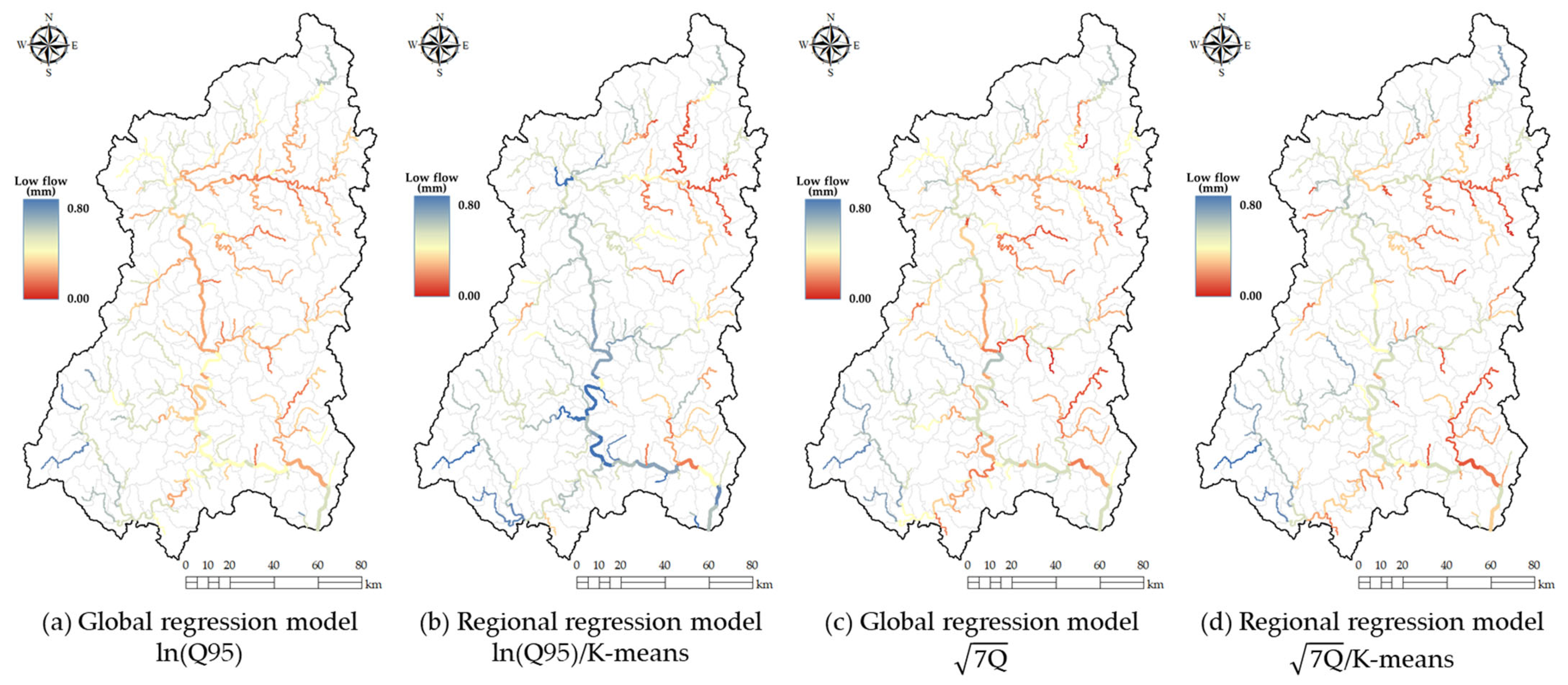
The spatial distribution of low-flow estimates was derived using both global and regional regression models for ln(Q95) and $\sqrt{7\mathrm{Q}}$. Figure 13 presents the predicted low-flow conditions along the river network, comparing results from the global regression model and the regional regression model developed using K-means clustering.

When ln(Q95) is considered a low-flow measure, the global regression model (Figure 13a) provides a broad-scale estimation of low flow across the watershed. However, the regional model (Figure 13b) shows a more detailed spatial differentiation, capturing localized variations in hydrological response. The regional regression model produces more distinct spatial contrasts, particularly in areas where elevation, slope, and seasonal precipitation effects are more pronounced. The ability to account for regional hydrological characteristics enhances the accuracy of low-flow predictions, reducing the overgeneralization observed in the global model.

In case of the $\sqrt{7\mathrm{Q}}$, a similar pattern is observed. The global regression model (Figure 13c) provides a general trend of low-flow distribution but lacks finer spatial differentiation. The regional model (Figure 13d) improves the representation of spatial variability by incorporating cluster-specific hydrological controls. Notably, the regional model highlights localized variations in base-flow conditions, which are less apparent in the global approach. These differences suggest that regional models may be more effective in capturing hydrologically distinct sub-regions, leading to a better representation of low-flow spatial distribution.

These results explain the importance of using a regional approach for low-flow estimation, particularly in large-scale watersheds where climatic and geomorphological heterogeneity influences hydrological response. The regional regression model not only improves prediction accuracy but also provides a spatially refined representation of low-flow patterns, making it a more suitable tool for watershed-scale water resource management.

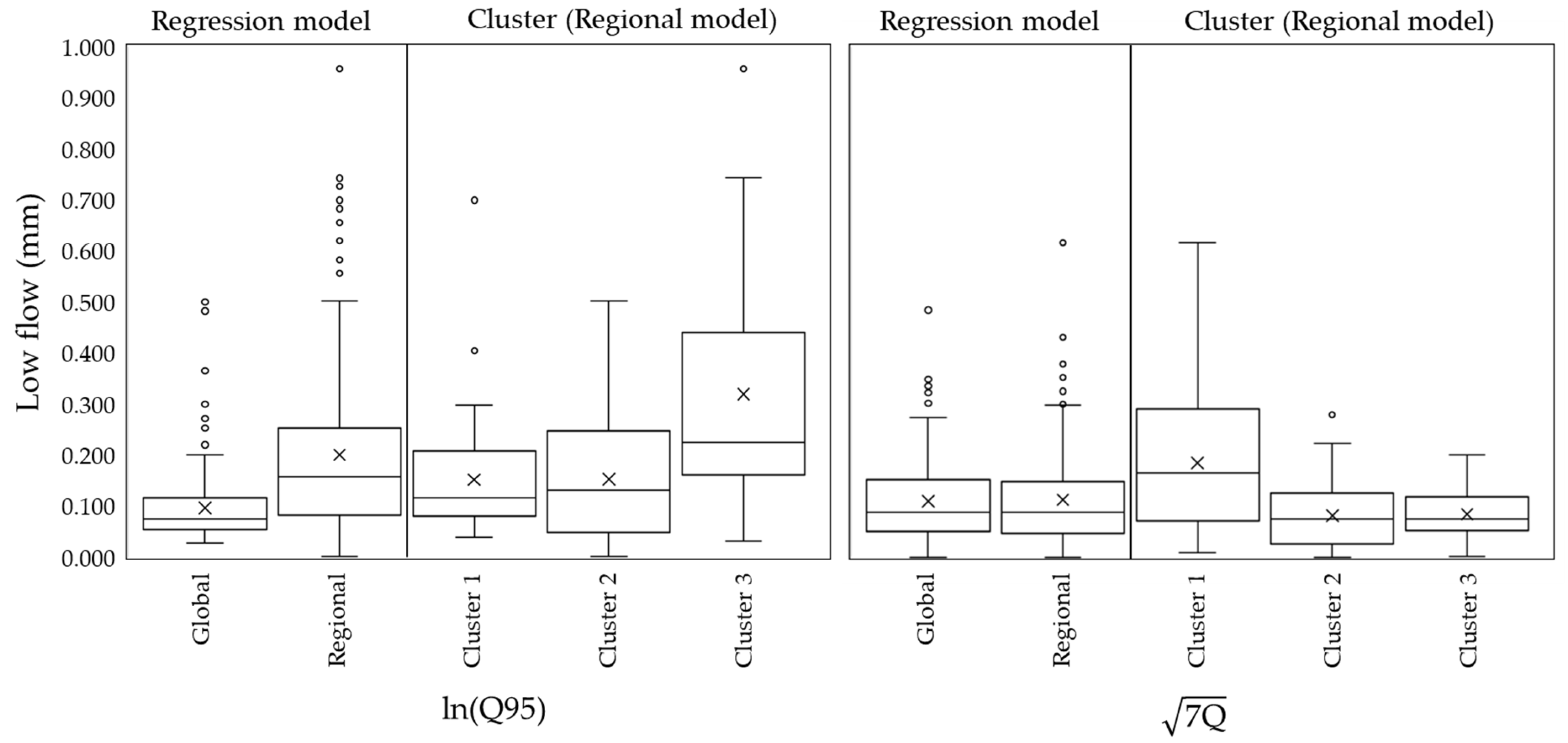
A box plot analysis was conducted to further evaluate the performance of the global and regional regression models. Figure 14 presents the distribution of low-flow estimates derived from the global and regional regression models for ln(Q95) and $\sqrt{7\mathrm{Q}}$. The boxplots illustrate the variability in low-flow predictions across different modeling approaches. The “Global” and “Regional” categories represent the outcomes of global and regional regression models, respectively, while “Cluster 1”, “Cluster 2”, and “Cluster 3” correspond to the results of the regional regression model, stratified by clusters.

For ln(Q95), the global regression model exhibited a relatively narrow interquartile range, indicating constrained predictions with limited responsiveness to local variability. In contrast, the regional regression model demonstrated a wider range and a higher median value, suggesting the improved representation of hydrological differences within the watershed. Among the cluster-based models, Cluster 3 exhibited the highest median value and the widest distribution range, showing its distinct hydrological characteristics compared to Clusters 1 and 2. These results demonstrate the effectiveness of the regionalization approach in identifying hydrologically distinct sub-watersheds and enhancing predictive accuracy. A similar trend was observed for $\sqrt{7\mathrm{Q}}$. The global regression model produced predictions with low variability and a more restricted distribution, whereas the regional regression model exhibited improved variability and accuracy in low-flow predictions. Further analysis of cluster-based models revealed that Cluster 3 displayed the widest distribution range of predicted low-flow values. This finding suggests that certain regions are more strongly influenced by localized climatic and topographic factors, reinforcing the necessity of regional models in capturing these characteristics.

A comparative analysis of ln(Q95) and $\sqrt{7\mathrm{Q}}$ within the same clusters provided further insights into the effectiveness of regional regression models. The regression equations for each model indicated that the coefficients of key explanatory variables varied depending on the selected low-flow index, reflecting differences in their relative importance. The ln(Q95) model exhibited a large absolute value for the intercept, along with high coefficients for precipitation, runoff-generation, and topographic factors, indicating that variations in climatological variables have a significant impact on low-flow characteristics. In contrast, the $\sqrt{7\mathrm{Q}}$ regression model showed a smaller absolute intercept value and relatively lower coefficients for climatological variables, suggesting lower sensitivity to these factors. Furthermore, an analysis of variable changes across indices revealed that the decline rate of precipitation coefficients was more pronounced than that of the runoff curve number or topographic variables. This finding suggests that, compared to ln(Q95), the $\sqrt{7\mathrm{Q}}$ model became more dependent on geomorphological factors and less dependent on climatic variables (

Table 2. Selected regression equations for low-flow inference based on the best-performing models.

Measure	Regression Model		Equation
ln(Q95)	Global		(0.0016 × P) + (−0.0591 × Smean) + (0.0045 × Emean) + (0.0637 × CL) + (1.9695 × WCR) − 4.8722
	Regional	Cluster 1	(0.0017 × P) + (0.0018 × Emax) + (0.0243 × RCN) + (−0.0301 × Smean) + (0.0010 × Area) − 6.9045
		Cluster 2	(0.0028 × Pw) + (−0.0238 × Emin) − 2.9139
		Cluster 3	(0.0024 × P) + (0.1024 × RCN) + (−0.0029 × Area) − 10.5934
$\sqrt{7\mathrm{Q}}$	Global		(0.0003 × P) + (0.0004 × Emax) + (0.0069 × RCN) + (−0.0093 × Smean) − 0.5348
	Regional	Cluster 1	(0.0004 × P) + (0.0004 × Emax) + (0.0069 × RCN) + (−0.0097 × Smean) + (0.0002 × Area) − 0.6707
		Cluster 2	(0.0001 × P) + (−0.0164 × Smean) + 0.6011
		Cluster 3	(0.0002 × P) + (0.0119 × RCN) − 0.7125

). These findings are consistent with those of Smakhtin [3], Vogel and Kroll [7], and Fenicia et al. [29], who reported a strong linkage between base-flow characteristics, watershed runoff, and precipitation patterns, emphasized the significant role of topographic factors in base-flow processes and the persistence of low flows, and argued that topographic and soil properties may exert a more critical influence on low-flow characteristics than long-term climatic factors, respectively. These studies may help explain the varying dependence of climatological variables on the two different measures of low flow.

4. Conclusions

This study investigated the effectiveness of low-flow regionalization for estimating low flow in a large-scale watershed with numerous ungauged sites. The regionalization was performed by integrating climatological variables and low-flow measures. Hydrologically homogeneous regions within the Nakdong River Basin were delineated using Ward’s method and K-means clustering to capture spatial variability in climatological variables and examine the correlation between the variables and low measures. The correlation was established through cluster-specific regression models developed to estimate Q95 and 7Q incorporating statistical transformations to improve prediction accuracy. The proposed methodology offered a sophisticated tool for low-flow prediction, particularly in ungauged basins where direct hydrological observations are scarce.

The results revealed that log and square-root transformations improved the predictive accuracy of regression models. In the case of Q95 estimation, the log-transformed regression model consistently yielded the highest predictive performance across most clusters, suggesting that Q95 follows a right-skewed distribution requiring logarithmic scaling for accurate modeling. Meanwhile, square-root transformation was more effective for 7Q estimation, likely due to its ability to balance skewness while preserving hydrological relationships. These findings provide the importance of applying appropriate statistical transformations when developing regression models for low-flow estimation.

Furthermore, the comparative analysis between regional and global models revealed that regional models exhibited higher predictive accuracy, as indicated by higher adjusted R² values and lower MSE across all clusters. The superior performance of regional models suggests that delineating hydrologically homogeneous regions provides a more refined approach to -low estimation, effectively capturing spatial variations in climatological and geomorphological controls. This study also identified key variables influencing low flow, with precipitation, elevation, mean slope, and the runoff curve number emerging as dominant predictors across different clusters. These findings reinforce the need for regionally tailored regression models that consider the unique hydrological characteristics of each sub-basin.

Overall, this study provides a practical framework for the estimation of low flow that can be a possible application in water resource management. The proposed methodology can infer the condition of low flow extended to ungauged basins and offer a reliable tool for hydrological predictions in data-scarce regions. Further improvement of regionalization techniques and model integration strategies will enhance the robustness of low-flow estimation contributing to the sustainability of water management practices.