


Application of a Multi-Teacher Distillation Regression Model Based on Clustering Integration and Adaptive Weighting in Dam Deformation Prediction


Abstract
1. Introduction
- A multi-teacher distillation framework for regression problems is proposed. Traditional knowledge distillation methods have certain limitations when dealing with regression problems. We provide a new paradigm for this field. With the help of our framework, it is possible to provide the student network with richer and more comprehensive knowledge information.
- We adopted a clustering integration method based on information theory to reduce the number of redundant and low-precision teacher networks. This avoids knowledge redundancy and conflicts caused by too many teacher networks, further enhancing the performance and stability of the model.
- We propose of a novel weighted loss function for regression to guide the student network. Different weights are assigned according to the performance of different teacher networks, enabling the student network to pay more attention to the knowledge content of high-quality teachers during the learning process.
- Our method was applied to a concrete-faced rockfill dam in Guizhou province, China. The results show that, through our distillation algorithm, the prediction accuracy (MSE) of the student network can be effectively reduced by 40% to 73%. Compared with other knowledge distillation methods, our method has higher accuracy and practicality.
2. Related Works
2.1. HST Statistical Model
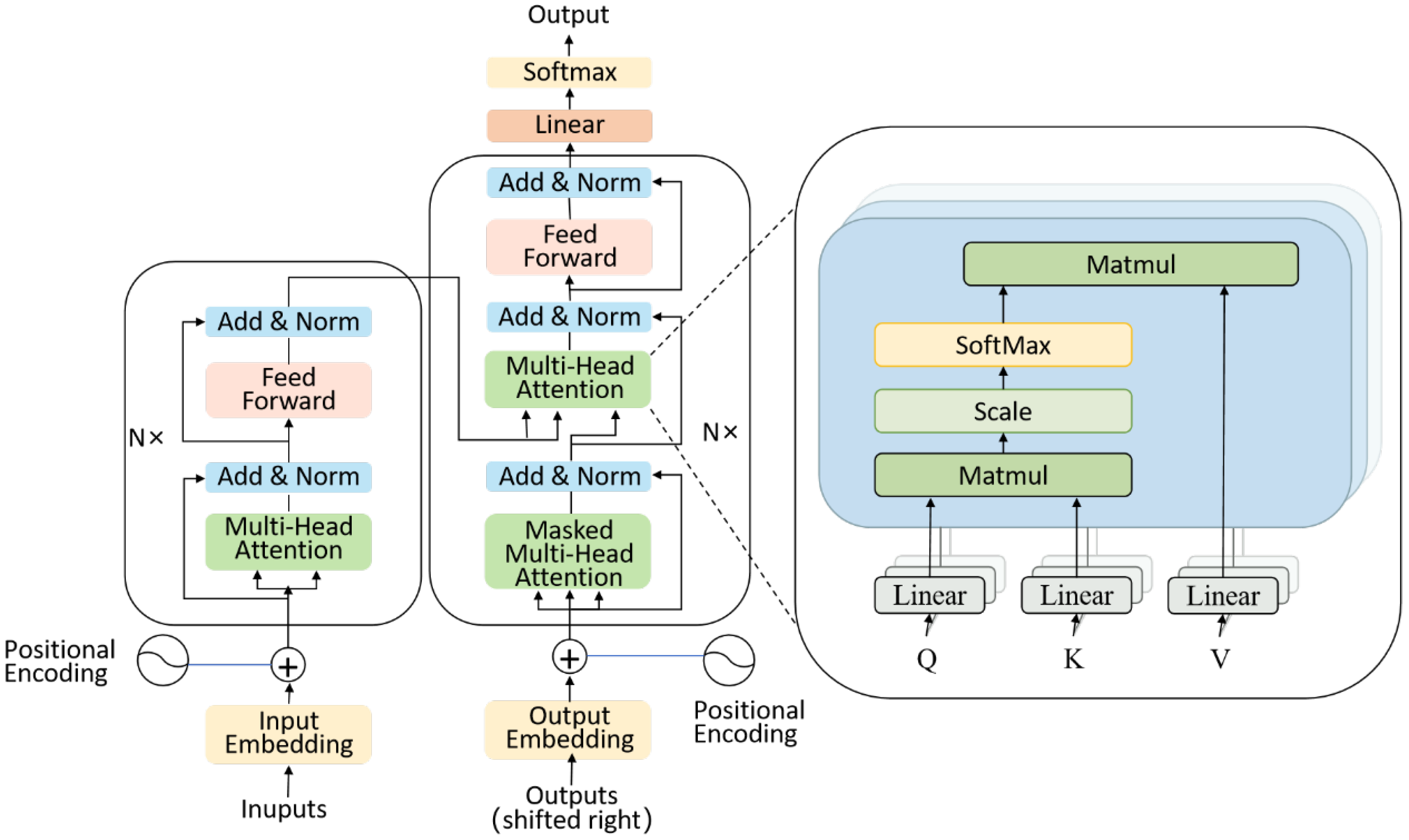
2.2. Transformer Model
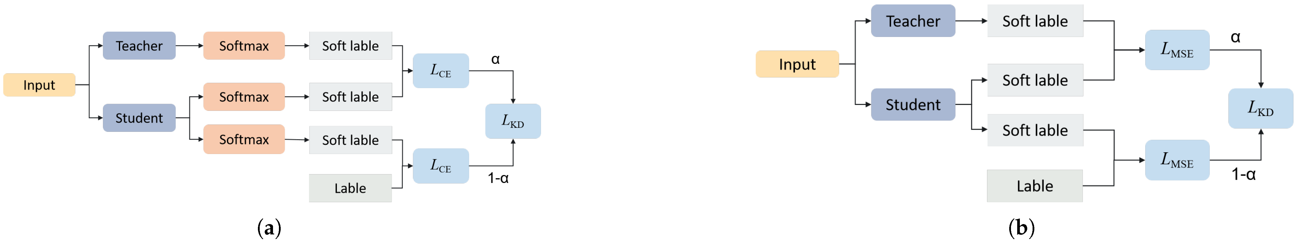
2.3. Multi-Teacher Knowledge Distillation
- Teacher model training: Multiple teacher models are trained independently. Each teacher model may be based on a different model architecture or a different training subset, ensuring that they possess unique knowledge and capabilities.
- Teacher model integration: in multi-teacher distillation, weighted averaging of the prediction results is usually adopted to ensure more accurate knowledge transfer.
- Student model training: The student model is trained to mimic the outputs of multiple teacher models as closely as possible. In classification tasks, the cross-entropy loss function is commonly used to measure the consistency between the outputs of the student model and the teacher models so as to achieve efficient knowledge transfer.
2.4. The Basic Concept of Information Entropy
3. Regression Method Based on Multi-Teacher Distillation
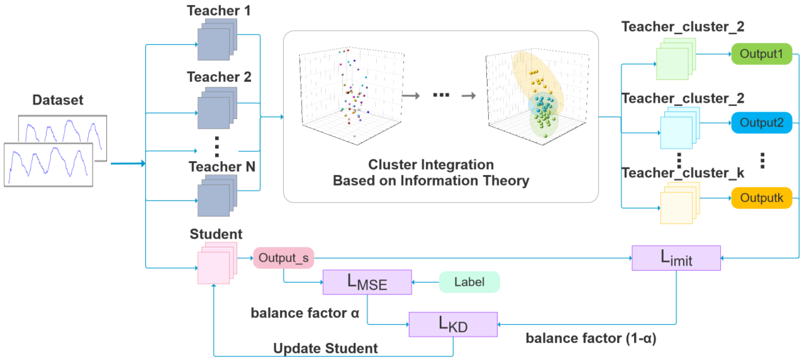
3.1. Method Overview
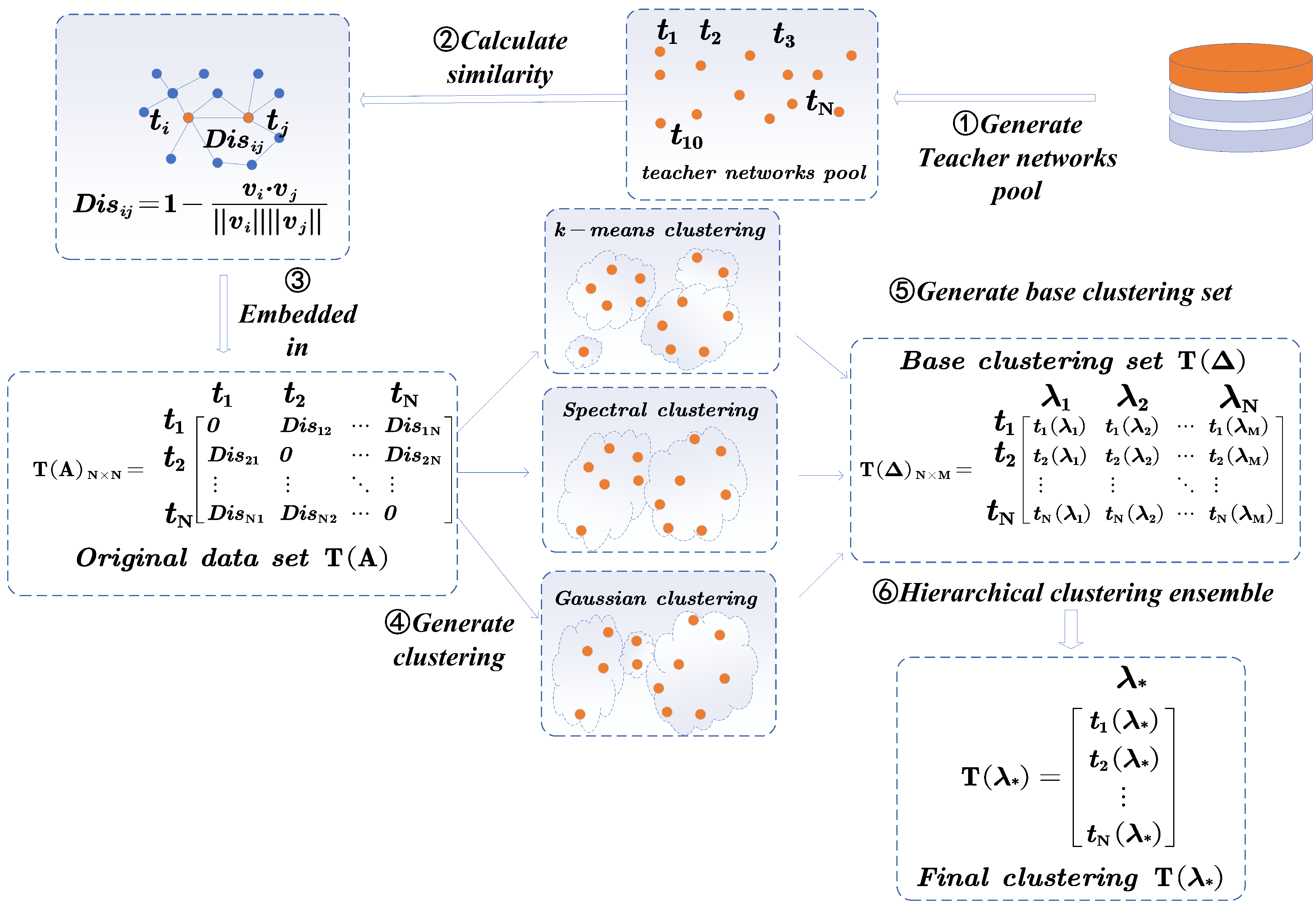
3.2. Multi-Teacher Network Clustering Ensemble Based on Information Theory
| Algorithm 1 Multi-teacher clustering ensemble based on information theory. |
|
3.3. Knowledge Distillation
4. Results
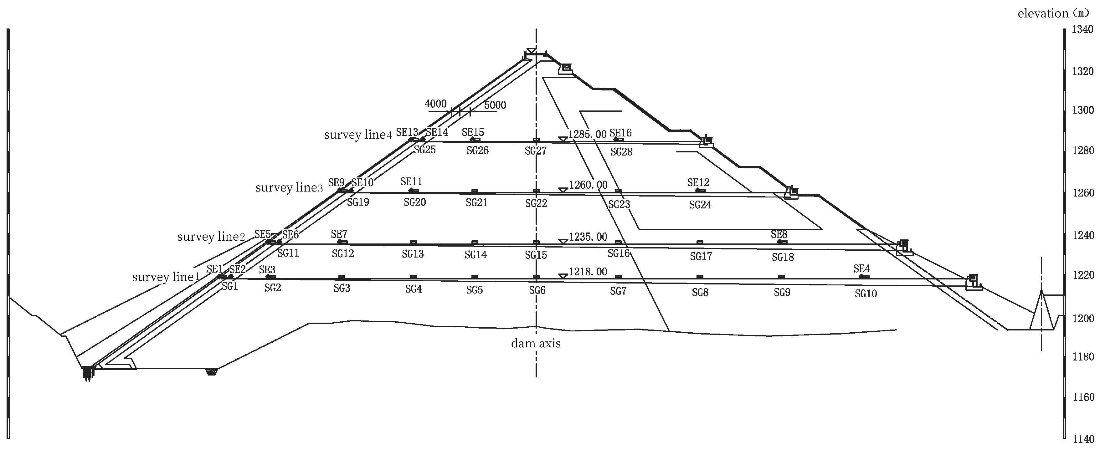
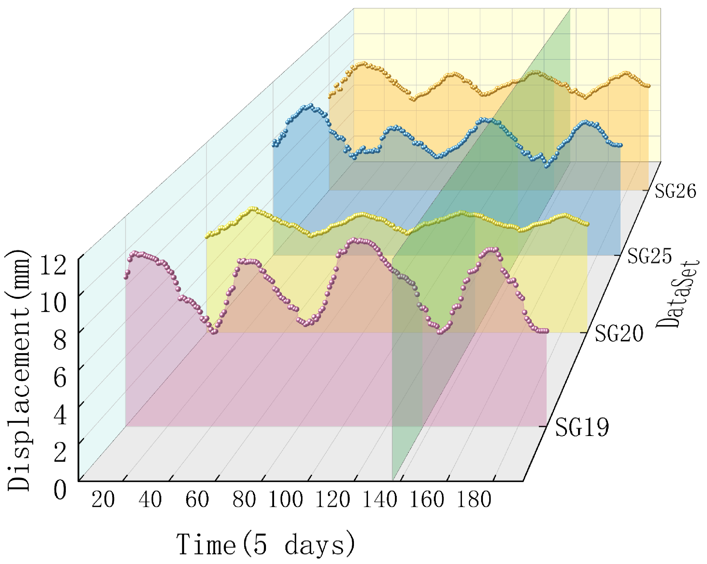
4.1. Project Overview
4.2. Evaluation Metrics
4.3. Experimental Settings
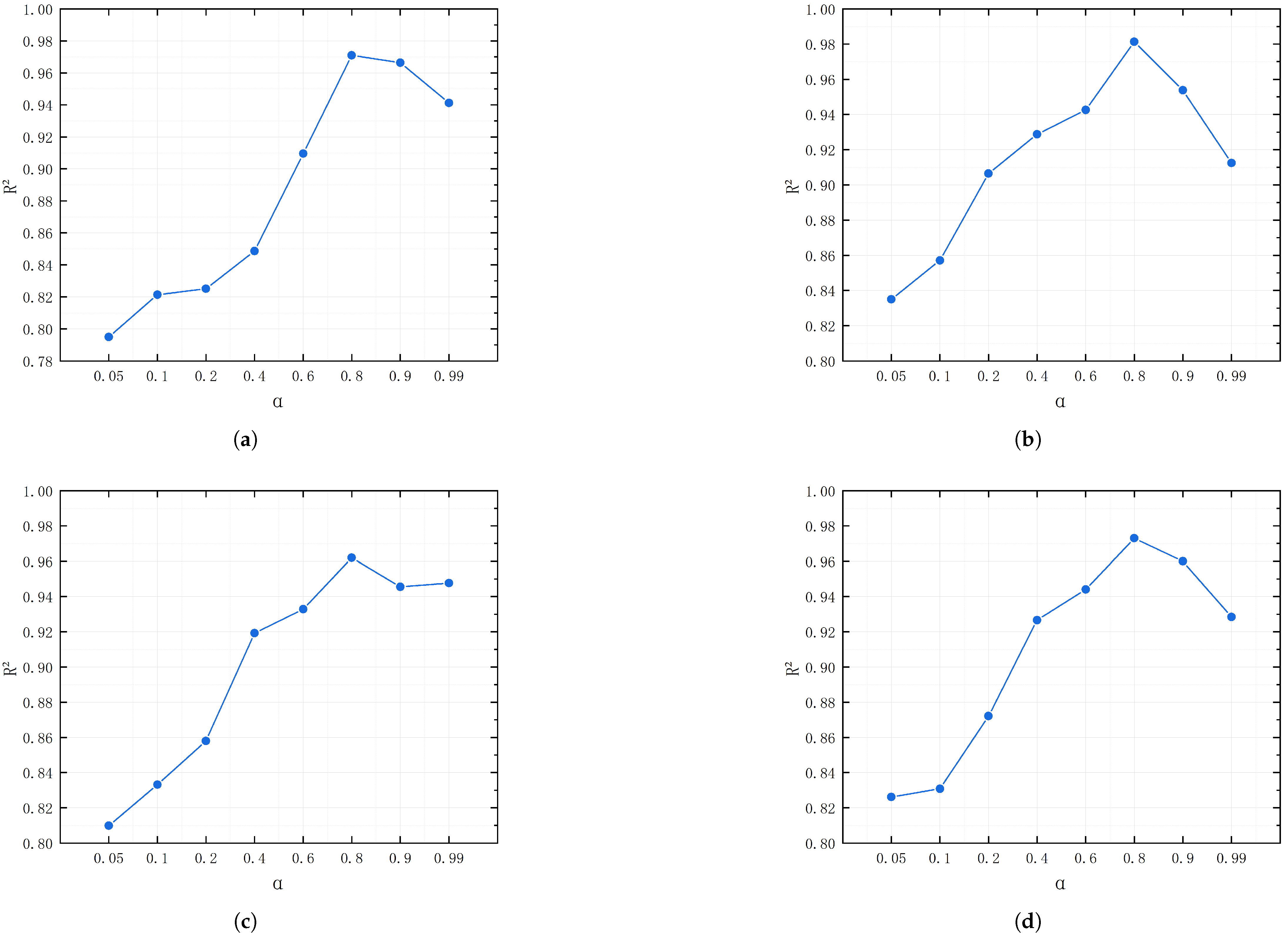
4.4. Parameter Sensitivity Experiment
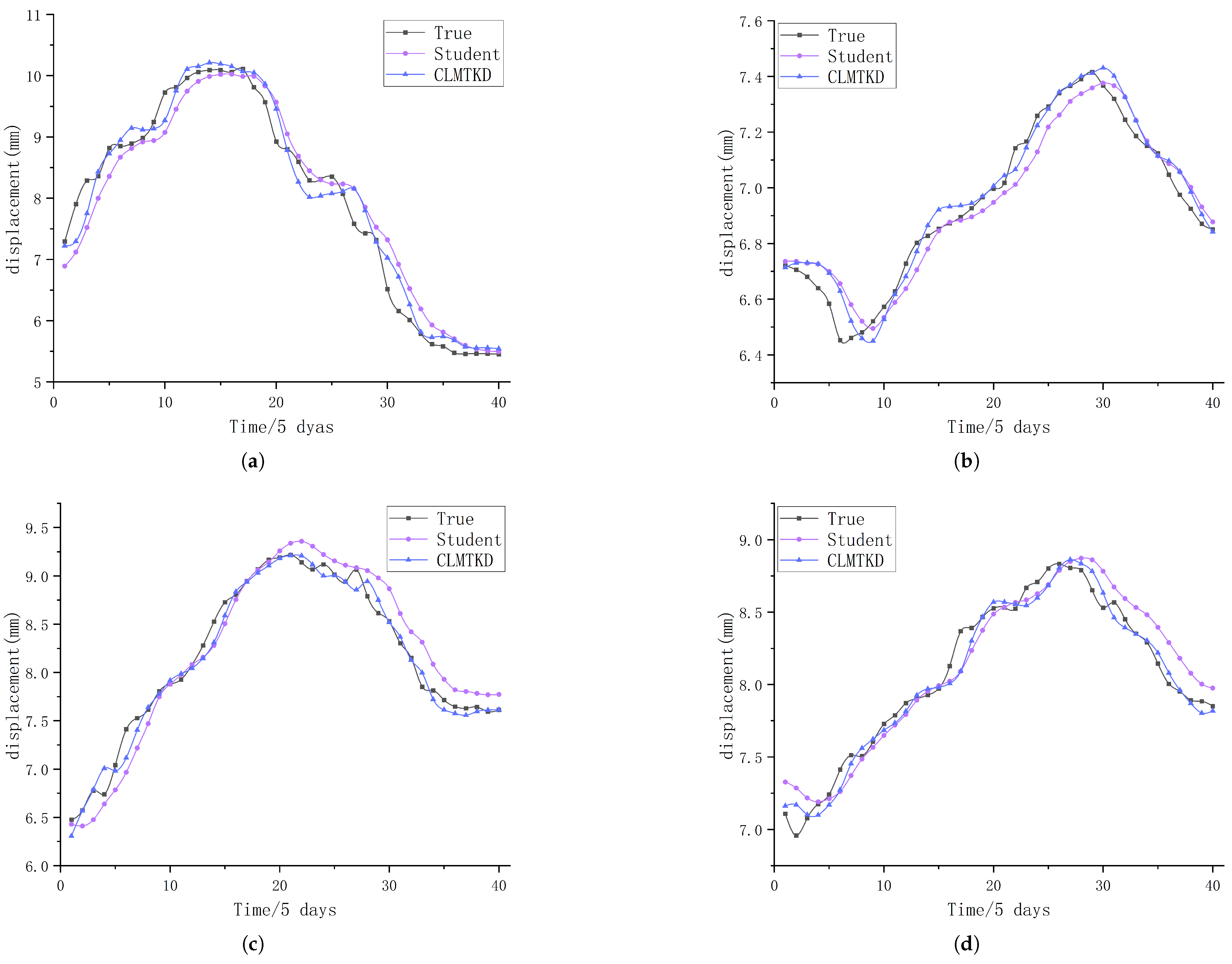
4.5. Distillation Performance Evaluation
4.6. Comparative Experiment
5. Conclusions
Author Contributions
Funding
Data Availability Statement
Conflicts of Interest
References
- Aydemir, A. Modified risk assessment tool for embankment dams: Case study of three dams in Turkey. Civ. Eng. Environ. Syst. 2017, 34, 53–67. [Google Scholar] [CrossRef]
- Sivasuriyan, A. Health assessment of dams under various environmental conditions using structural health monitoring techniques: A state-of-art review. In Environmental Science and Pollution Research; Springer Nature: Berlin/Heidelberg, Germany, 2022; pp. 1–12. [Google Scholar]
- Yang, J. An intelligent prediction model of settlement deformation for the earth-rock dam. In Proceedings of the 2021 International Conference on Artificial Intelligence, Big Data and Algorithms (CAIBDA), Xi’an, China, 28–30 May 2021; pp. 198–201. [Google Scholar]
- Wang, Q. Research on dam deformation prediction based on variable weight combination model. In Proceedings of the 2024 4th International Conference on Neural Networks, Information and Communication (NNICE), Guangzhou, China, 19–21 January 2024; pp. 900–903. [Google Scholar]
- Luo, C. Research on Dam Deformation Prediction Model Based on Wavelet Neural Network. In Proceedings of the 2021 3rd International Conference on Applied Machine Learning (ICAML), Changsha, China, 23–25 July 2021; pp. 362–365. [Google Scholar]
- Zhu, Y. Automatic damage detection and diagnosis for hydraulic structures using drones and artificial intelligence techniques. Remote Sens. 2023, 15, 615. [Google Scholar] [CrossRef]
- Zhu, M. Optimized multi-output LSSVR displacement monitoring model for super high arch dams based on dimensionality reduction of measured dam temperature field. Eng. Struct. 2022, 268, 114686. [Google Scholar] [CrossRef]
- Mata, J. Constructing statistical models for arch dam deformation. Struct. Control Health Monit. 2014, 21, 423–437. [Google Scholar] [CrossRef]
- Chen, R. Construction and selection of deformation monitoring model for high arch dam using separate modeling technique and composite decision criterion. Struct. Health Monit. 2024, 23, 2509–2530. [Google Scholar] [CrossRef]
- Wu, B. A Multiple-Point Deformation Monitoring Model for Ultrahigh Arch Dams Using Temperature Lag and Optimized Gaussian Process Regression. Struct. Control Health Monit. 2024, 2024, 2308876. [Google Scholar] [CrossRef]
- Xing, Y. Research on dam deformation prediction model based on optimized SVM. Processes 2022, 10, 1842. [Google Scholar] [CrossRef]
- Li, X. An approach using random forest intelligent algorithm to construct a monitoring model for dam safety. Eng. Comput. 2021, 37, 39–56. [Google Scholar] [CrossRef]
- Hipni, A. Daily forecasting of dam water levels: Comparing a support vector machine (SVM) model with adaptive neuro fuzzy inference system (ANFIS). Water Resour. Manag. 2013, 27, 3803–3823. [Google Scholar] [CrossRef]
- Yang, D. A concrete dam deformation prediction method based on LSTM with attention mechanism. IEEE Access 2020, 8, 185177–185186. [Google Scholar] [CrossRef]
- Yang, J. A CNN-LSTM model for tailings dam risk prediction. IEEE Access 2020, 8, 206491–206502. [Google Scholar]
- Jiedeerbieke, M. Gravity Dam Deformation Prediction Model Based on I-KShape and ZOA-BiLSTM. IEEE Access 2024, 12, 50710–50722. [Google Scholar] [CrossRef]
- Su, Y. Dam deformation interpretation and prediction based on a long short-term memory model coupled with an attention mechanism. Appl. Sci. 2021, 11, 6625. [Google Scholar] [CrossRef]
- Zhou, Y. Multi-expert attention network for long-term dam displacement prediction. Adv. Eng. Informatics 2023, 57, 102060. [Google Scholar]
- Wang, X. Study on MPGA-BP of gravity dam deformation prediction. Math. Probl. Eng. 2017, 2017, 2586107. [Google Scholar]
- Hinton, G. Distilling the knowledge in a neural network. arXiv 2015, arXiv:1503.02531. [Google Scholar]
- Sun, T. Explainability-based knowledge distillation. Pattern Recognit. 2025, 159, 111095. [Google Scholar]
- Chu, Y. Bi-directional contrastive distillation for multi-behavior recommendation. In Joint European Conference on Machine Learning and Knowledge Discovery in Databases; Springer International Publishing: Cham, Switzerland, 2022; pp. 491–507. [Google Scholar]
- Lopez-Paz, D. Unifying distillation and privileged information. arXiv 2015, arXiv:1511.03643. [Google Scholar]
- Yuan, Y. The Impact of Knowledge Distillation on the Energy Consumption and Runtime Efficiency of NLP Models. In Proceedings of the IEEE/ACM 3rd International Conference on AI Engineering-Software Engineering for AI, Lisbon, Portugal, 14–15 April 2024; pp. 129–133. [Google Scholar]
- Léger, P. Hydrostatic, temperature, time-displacement model for concrete dams. J. Eng. Mech. 2007, 133, 267–277. [Google Scholar]
- Vaswani, A.; Shazeer, N.; Parmar, N.; Uszkoreit, J.; Jones, L.; Gomez, A.N.; Kaiser, Ł.; Polosukhin, I. Attention is all you need. Adv. Neural Inf. Process. Syst. 2017, 30, 5998–6008. [Google Scholar]
- Xu, C. A financial time-series prediction model based on multiplex attention and linear transformer structure. Appl. Sci. 2023, 13, 5175. [Google Scholar] [CrossRef]
- Ahmed, S. Transformers in time-series analysis: A tutorial. Circuits Syst. Signal Process. 2023, 42, 7433–7466. [Google Scholar] [CrossRef]
- Sasal, L. W-transformers: A wavelet-based transformer framework for univariate time series forecasting. In Proceedings of the 2022 21st IEEE International Conference on Machine Learning and Applications (ICMLA), Nassau, Bahamas, 12–14 December 2022; pp. 671–676. [Google Scholar]
- Wen, Q. Transformers in time series: A survey. arXiv 2022, arXiv:2202.07125. [Google Scholar]
- Hittawe, M.M. Stacked Transformer Models for Enhanced Wind Speed Prediction in the Red Sea. In Proceedings of the 2024 IEEE 22nd International Conference on Industrial Informatics (INDIN), Beijing, China, 18–20 August 2024; pp. 1–7. [Google Scholar]
- Jiang, W. Applicability analysis of transformer to wind speed forecasting by a novel deep learning framework with multiple atmospheric variables. Appl. Energy 2024, 353, 122155. [Google Scholar] [CrossRef]
- Lin, Y. ATMKD: Adaptive temperature guided multi-teacher knowledge distillation. Multimed. Syst. 2024, 30, 292. [Google Scholar] [CrossRef]
- Zhang, H. Adaptive multi-teacher knowledge distillation with meta-learning. In Proceedings of the 2023 IEEE International Conference on Multimedia and Expo (ICME), Brisbane, Australia, 10–14 July 2023; pp. 1943–1948. [Google Scholar]
- Sarıyıldız, M.B. UNIC: Universal Classification Models via Multi-teacher Distillation. In European Conference on Computer Vision; Springer Nature: Cham, Switzerland, 2024; pp. 353–371. [Google Scholar]
- Li, R. Cross-View Gait Recognition Method Based on Multi-Teacher Joint Knowledge Distillation. Sensors 2023, 23, 9289. [Google Scholar] [CrossRef]
- Yang, Y. MKDAND: A network flow anomaly detection method based on multi-teacher knowledge distillation. In Proceedings of the 2022 16th IEEE International Conference on Signal Processing (ICSP), Beijing, China, 21–24 October 2022; Volume 1, pp. 314–319. [Google Scholar]
- Pham, C. Collaborative multi-teacher knowledge distillation for learning low bit-width deep neural networks. In Proceedings of the IEEE/CVF Winter Conference on Applications of Computer Vision, Waikoloa, HI, USA, 3–7 January 2023; pp. 6435–6443. [Google Scholar]
- Ye, X. Knowledge distillation via multi-teacher feature ensemble. IEEE Signal Process. Lett. 2024, 31, 566–570. [Google Scholar] [CrossRef]
- Wu, C. One teacher is enough? Pre-trained language model distillation from multiple teachers. arXiv 2021, arXiv:2106.01023. [Google Scholar]
- Zhang, J. Badcleaner: Defending backdoor attacks in federated learning via attention-based multi-teacher distillation. IEEE Trans. Dependable Secur. Comput. 2024, 21, 4559–4573. [Google Scholar] [CrossRef]
- Bai, L. An information-theoretical framework for cluster ensemble. IEEE Trans. Knowl. Data Eng. 2018, 31, 1464–1477. [Google Scholar] [CrossRef]
- Lee, K. Fast and accurate facial expression image classification and regression method based on knowledge distillation. Appl. Sci. 2023, 13, 6409. [Google Scholar] [CrossRef]
- Bai, S. An empirical evaluation of generic convolutional and recurrent networks for sequence modeling. arXiv 2018, arXiv:1803.01271. [Google Scholar]
- Saputra, M.R.U. Distilling knowledge from a deep pose regressor network. In Proceedings of the IEEE/CVF International Conference on Computer Vision, Seoul, Republic of Korea, 27 October–2 November 2019; pp. 263–272. [Google Scholar]
- Chen, G.; Choi, W.; Yu, X.; Han, T.; Chandraker, M. Learning efficient object detection models with knowledge distillation. Adv. Neural Inf. Process. Syst. 2017, 30, 742–751. [Google Scholar]
- Takamoto, M. An efficient method of training small models for regression problems with knowledge distillation. In Proceedings of the 2020 IEEE Conference on Multimedia Information Processing and Retrieval (MIPR), Shenzhen, China, 6–8 August 2020; pp. 67–72. [Google Scholar]

| Symbol | Description |
|---|---|
| The feature value of the h-th base clustering | |
| D(v) | The domain of variable (feature) v |
| The clustering label of | |
| The h-th base clustering set | |
| The l-th cluster in | |
| S ⊆ T | A cluster composed of multiple objects in T |
| A set composed of clusters S where is the l-th cluster | |
| The set composed of the objects in T, which is defined as a partition | |
| The partition result formed by the final clusters | |
| k | The number of clusters in partition |
| The final clustering feature vector |
| Network | #Params | FLOPs |
|---|---|---|
| Transformer | 87,007 | 8735 |
| TCN | 20.735 M | 0.9928 M |
| Dataset | Model | MSE (mm) | RMSE (mm) | MAE (mm) | MAPE | |
|---|---|---|---|---|---|---|
| TeacherCL1 | 0.06049 | 0.24595 | 0.18483 | 2.36203 | 0.97679 | |
| TeacherCL2 | 0.09914 | 0.31487 | 0.25275 | 3.35216 | 0.96196 | |
| SG19 | TeacherCL3 | 0.10856 | 0.32949 | 0.25964 | 3.57259 | 0.95834 |
| Student | 0.13955 | 0.37357 | 0.29399 | 3.88849 | 0.94644 | |
| CLMTKD | 0.07578 | 0.27527 | 0.21325 | 2.77232 | 0.97092 | |
| TeacherCL1 | 0.00267 | 0.0513 | 0.04072 | 0.59478 | 0.96749 | |
| TeacherCL2 | 0.00317 | 0.05634 | 0.04432 | 0.64194 | 0.96088 | |
| SG20 | TeacherCL3 | 0.00507 | 0.07117 | 0.05386 | 0.78496 | 0.93758 |
| Student | 0.00520 | 0.07210 | 0.05923 | 0.85757 | 0.93594 | |
| CLMTKD | 0.00308 | 0.05554 | 0.04265 | 0.62291 | 0.96199 | |
| TeacherCL1 | 0.01446 | 0.12027 | 0.09045 | 1.14168 | 0.97692 | |
| TeacherCL2 | 0.03564 | 0.18879 | 0.15237 | 1.93899 | 0.94313 | |
| SG25 | TeacherCL3 | 0.03783 | 0.19449 | 0.15885 | 1.98612 | 0.93964 |
| Student | 0.04463 | 0.21127 | 0.17393 | 2.18014 | 0.92878 | |
| CLMTKD | 0.01171 | 0.10819 | 0.07837 | 0.98788 | 0.98132 | |
| TeacherCL1 | 0.01018 | 0.10090 | 0.08128 | 1.01031 | 0.96411 | |
| TeacherCL2 | 0.01446 | 0.12026 | 0.09729 | 1.21837 | 0.94901 | |
| SG26 | TeacherCL3 | 0.01482 | 0.12174 | 0.09554 | 1.17603 | 0.94775 |
| Student | 0.02176 | 0.14753 | 0.12029 | 1.50459 | 0.92327 | |
| CLMTKD | 0.00766 | 0.08754 | 0.06781 | 0.84433 | 0.97298 |
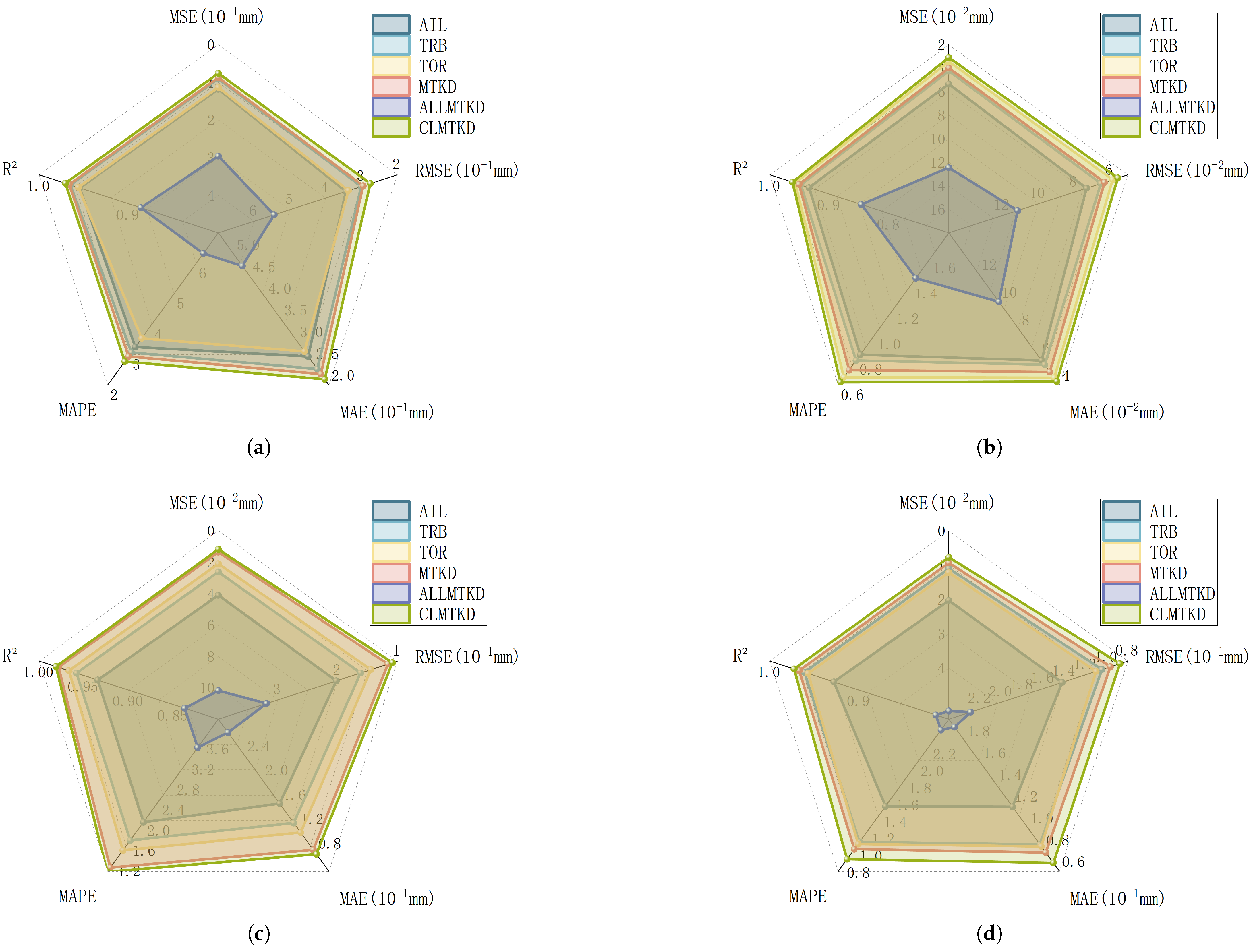
| Dataset | Model | MSE (mm) | RMSE (mm) | MAE (mm) | MAPE | |
|---|---|---|---|---|---|---|
| SG19 | AIL | 0.11798 | 0.34348 | 0.26597 | 3.25020 | 0.954724 |
| TBR | 0.09040 | 0.30066 | 0.23679 | 3.07238 | 0.965308 | |
| TOR | 0.11135 | 0.33638 | 0.27738 | 3.53747 | 0.95658 | |
| MTKD | 0.08714 | 0.29520 | 0.22549 | 2.94286 | 0.96656 | |
| ALLMTKD | 0.29588 | 0.54394 | 0.47393 | 6.32527 | 0.88645 | |
| CLMTKD | 0.07578 | 0.27527 | 0.21325 | 2.77232 | 0.97092 | |
| SG20 | AIL | 0.00534 | 0.07307 | 0.05780 | 0.83995 | 0.93421 |
| TBR | 0.00423 | 0.06504 | 0.05466 | 0.79410 | 0.94788 | |
| TOR | 0.00432 | 0.05848 | 0.04533 | 0.66193 | 0.95786 | |
| MTKD | 0.00398 | 0.06305 | 0.04952 | 0.71876 | 0.95102 | |
| ALLMTKD | 0.01245 | 0.11157 | 0.10012 | 1.44319 | 0.84661 | |
| CLMTKD | 0.00308 | 0.05554 | 0.04265 | 0.62291 | 0.96199 | |
| SG25 | AIL | 0.04095 | 0.20237 | 0.16139 | 1.96994 | 0.93465 |
| TBR | 0.02605 | 0.16139 | 0.12953 | 1.61069 | 0.95844 | |
| TOR | 0.02077 | 0.14413 | 0.11386 | 1.41403 | 0.96685 | |
| MTKD | 0.01336 | 0.11561 | 0.08560 | 1.07310 | 0.97867 | |
| ALLMTKD | 0.10177 | 0.31900 | 0.27808 | 3.44080 | 0.83762 | |
| CLMTKD | 0.01171 | 0.10819 | 0.07837 | 0.98788 | 0.98132 | |
| SG26 | AIL | 0.02030 | 0.14246 | 0.11936 | 1.47008 | 0.92845 |
| TBR | 0.01038 | 0.10186 | 0.07854 | 0.97147 | 0.96342 | |
| TOR | 0.01212 | 0.11010 | 0.08304 | 1.02446 | 0.95727 | |
| MTKD | 0.00932 | 0.09648 | 0.07726 | 0.96672 | 0.96718 | |
| ALLMTKD | 0.05261 | 0.22937 | 0.19274 | 2.32723 | 0.81451 | |
| CLMTKD | 0.00766 | 0.08754 | 0.06781 | 0.84433 | 0.97298 |
Disclaimer/Publisher’s Note: The statements, opinions and data contained in all publications are solely those of the individual author(s) and contributor(s) and not of MDPI and/or the editor(s). MDPI and/or the editor(s) disclaim responsibility for any injury to people or property resulting from any ideas, methods, instructions or products referred to in the content. |
© 2025 by the authors. Licensee MDPI, Basel, Switzerland. This article is an open access article distributed under the terms and conditions of the Creative Commons Attribution (CC BY) license (https://creativecommons.org/licenses/by/4.0/).
Share and Cite
Guo, F.; Yuan, J.; Li, D.; Qin, X. Application of a Multi-Teacher Distillation Regression Model Based on Clustering Integration and Adaptive Weighting in Dam Deformation Prediction. Water 2025, 17, 988. https://doi.org/10.3390/w17070988
Guo F, Yuan J, Li D, Qin X. Application of a Multi-Teacher Distillation Regression Model Based on Clustering Integration and Adaptive Weighting in Dam Deformation Prediction. Water. 2025; 17(7):988. https://doi.org/10.3390/w17070988
Chicago/Turabian StyleGuo, Fawang, Jiafan Yuan, Danyang Li, and Xue Qin. 2025. "Application of a Multi-Teacher Distillation Regression Model Based on Clustering Integration and Adaptive Weighting in Dam Deformation Prediction" Water 17, no. 7: 988. https://doi.org/10.3390/w17070988
APA StyleGuo, F., Yuan, J., Li, D., & Qin, X. (2025). Application of a Multi-Teacher Distillation Regression Model Based on Clustering Integration and Adaptive Weighting in Dam Deformation Prediction. Water, 17(7), 988. https://doi.org/10.3390/w17070988