Abstract
Rainfall–runoff models are widely used in water management and flood forecasting. In this study, we present a rainfall–runoff model to forecast hourly flows based on an artificial neural network (ANN). This model was developed and applied to the Iton watershed (northwestern France) to solve the problems of nonlinearity in the rainfall–runoff relationship resulting from karst and complex hydrogeological behaviors. The model design required several steps during which we were able to identify the model parameters and create the database needed to perform the flow rate forecast. This work has resulted in an ANN model able to perform an efficient prediction up to a 48 h time horizon. These results confirm that ANN models can play an important role in forecasting the nonlinear rainfall–runoff relationship encountered in many watersheds.
1. Introduction
The use of artificial neural networks in the field of hydrology is becoming increasingly important. This technique has been applied in hydrological modeling successfully and showed significant computing power in several works dealing with rainfall–runoff modeling [1], especially in the field of flow forecasting [2,3,4,5]. The application of ANNs in hydrological modeling was discussed by the American Society of Civil Engineers (ASCE) in the working committee on the application of ANNs in hydrology [6]. The major advantages of ANN modeling are its nonparametric nature and simple adaptation to different types of data. However, the successful application of an ANN in hydrological modeling depends on the determination of the optimal structure of the ANN, the calibration phase, and procedures of decision making. In this paper, we present a rainfall–runoff model to forecast hourly flows based on artificial neural networks (ANNs) applied to the Iton watershed (northwest of France). The hydrological behavior of this watershed is strongly affected by karst hydrogeological behavior that involves a nonlinear rainfall–runoff relationship. The ANN model has been designed to forecast the flow rate at prediction horizons of 6, 12, 24, and 48 h. The results of this applied case study confirm that ANN models can provide a solution in flow rate forecasting for watersheds affected by karst or complex hydrogeological behavior. The first part of this paper presents the ANN including the general principles, multi-layered perceptron, design methodology, and performance assessment. The second part describes the case study. Finally, the third part presents and discusses the results and outputs of this research.
2. Artificial Neural Networks: Brief Review
2.1. General Principle
The ANN method requires the determination of the architecture, which includes the number of layers and number of artificial neurons in each layer and the activation functions associated with neurons. A neuron is characterized by its state, its connections with other neurons, and its activation function. The state is influenced by the input data, which are further transmitted to the whole neural network, layer after layer up to the output layer [7], through connections, eventually giving the ANN its global behavior.
The activation function (e.g., identity, logistic sigmoid, hyperbolic tangent…) is a mathematical function applied to entering signals for all the artificial neurons. It is user-defined and allows for the expression of the influence of a neuron on another one during information transfer [3]. The network performance can be greatly influenced by the type of activation function.
Multi-layered perceptrons (MLPs), or radial functions, are common ANN models when nonlinear relationships are simulated [8]. Following Lallahem and Mania (2003) [3], MLPs are among the most used and most sophisticated models. The training phase of an ANN consists of calculating and optimizing the information weight of the nonlinear relationship, between the input and output. This phase is iterative and is followed by two other phases: the test and validation phases. These last phases are crucial before the model runs.
2.2. Multi-Layered Perceptron
ANN simulates the principle of the human brain by managing the information flow from a training set [7,9,10,11]. It is a powerful tool which allows for the calculation and establishment of the nonlinearity of the input–output relationships of a system [11]. MLPs are widely used for hydrological prediction. They permit the transformation of the activation thresholds into a nonlinear response [12], thus reflecting the relationship between rainfall and the flow rate. These networks, with a unique connection type of “inter-layer”, keep the error propagation between neurons, as well as the calculation time, to a minimum. As a matter of fact, MLPs successively enclose an input layer, one (or several) hidden layer, and an output layer. These layers are interconnected by the weights Wij of their neurons (Figure 1) [11,12,13], but the neurons in the same layer are not connected. The ANN architecture is determined by the number of layers and the number of neurons per layer. The first layer receives input variables (Xi) through input neurons i, transforms them with the activation function f on the input neuron, and sends them to the neurons j of the first hidden layer. Typically, input neurons maintain input signals unchanged by utilizing identity activation functions. The hidden layer consists of processing neurons that receive weighted sums Sj (Equation (1)) from the input layer. These neurons apply a transformation using an activation function before passing the processed signals to the next layer, whether another hidden layer or the output layer, depending on the network’s architecture.
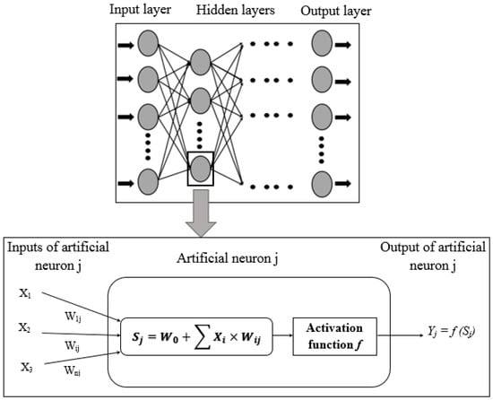
Figure 1.
General artificial neural network (interconnection of input, hidden, and output layers).
Sj is the pondered sum of the jth neuron; n is the number of input elements; Xi is the output value of the jth neuron of the precedent layer; Wij is the weight value between neurons i and j; and W0 is the bias. MLPs often work with only one hidden layer. It offers a sufficient degree of freedom and is similar to a nonlinear function [10,11,12,13,14]. No matter the number of hidden layers in an MLP, there exists one MLP with a unique hidden layer that produces the same quantity of errors [4]. In contrast, MLPs with a unique hidden layer show less complexity than other types of MLPs. They show less possible interconnections and, therefore, a more rapid convergence than the one produced by multiple-hidden-layer MLPs. Consequently, this study is limited to single-hidden-layer MLPs. The production equation in a three-layer MLP (n neurons in the input layer, m neurons in the hidden layer, and p neurons in the output layer) is as follows:
Yk is one of the system’s outputs; fk and fj are the activation functions of the neuron k of the output layer and the neuron j of the hidden layer, respectively; Wjk and Wij are the weights between the jth and the kth neurons of the output layer and between the ith and jth neurons, respectively; and W0 is the bias. Generally, the activation function is either the logistic sigmoid function or the hyperbolic tangent function [15]. The logistic sigmoid function is more frequently used [3] because this function is continuous, non-decreasing, differentiable, and bracketed and can introduce hydrological nonlinearity to an ANN model. Its mathematical representation is as follows:
S is the variable.
3. Methods
In an ANN, the observation of a hydrological system is conducted during the training phase. It is an iterative phase that consists of both the calculation and optimization of the information weight of the nonlinear relationship between rainfall and the flow rate. Its reliability depends on the ANN architecture, which differs from one system to another. In this study, the input variables, architecture determination of the adapted network, optimization of the network training, and use of a reliable validation methodology are crucial for the ANN model’s performance optimization.
Generally, not all of the system’s variables bring the same informative contribution. Therefore, it is interesting to select an input vector adequate for ANN modeling [16]. In order to determine the most informative variables (when compared to future flow rates Q(t + t0)), cross-correlation is applied. Subsequently, numerical experimentation (trial–error) is used: different combinations of rainfall and flow rates are studied. This aims at determining the optimum input variables for the ANN, in order to estimate the first deadline for flood prediction (Q(t + 6)). In fact, the selection of Q(t + 6)’s informative variables allows for the selection of future hydrology informative variables. In other words, Q(t + 6)’s explanatory variables represent the last historic variables that can explain Q(t + t0). This experiment is based on the following equation:
P is the rainfall; Q is the flow rate; and n and m are defined later in this article.
The most efficient determination of the ANN architecture is only achieved through experimental trials and depends on the case studied. Once input variables are chosen, the determination of the number of nodes (or neurons) in a hidden layer is automatically obtained using a statistic model. This defines the optimum number of hidden neurons for each iteration. The number of nodes in the output layer will be the flow rate at t + t0 (t0 shows the prediction horizon, PH).
The ANN architecture’s determination also consists of choosing the activation function for the nodes of hidden and output layers. The function used here is the sigmoid logistic function. The pretreatment of the function’s variables is necessary in order to take into account all the values (strong and weak) and to avoid sigmoid saturation with the database’s strong values. In fact, the direct application of the sigmoid function in pondered sums of the rainfall–flow rate inputs leads to information from weak numerical values (rainfall) being ignored compared to information from strong numerical values (flow rate). This treatment consists of normalizing the database (values between 0 and 1), thanks to the following equation:
X is the real value to normalize; Xmin is its minimum value; Xmax is its maximum value; and is the normalized value.
Neuronal networks are tools that (1) are highly nonlinear and (2) can learn how to model hydro-systems through examples chosen among a finite number of iterations. This data modeling considers iterative techniques of optimization (numerical algorithms) in order to facilitate ANN model adjustments. The most used technique for the calibration of ANNs is the Broyden–Fletcher–Goldfarb–Shanno (BFGS) algorithm. This algorithm demands a lot of memory and requires time-consuming computations. However, a small number of iterations can be used to calibrate an ANN, as a rapid convergence rate can be obtained.
ANN modeling considers three essential phases before its exploitation: training, test, and validation. ANN training necessitates historical data in order to calibrate flood prediction models. It calculates the neuronal interconnection weights of the different layers for the identification of the system. The training phase determines the quality of the non-finite ANN models with injected values (from the historical data) in the output layer and assesses the performance of the weights determined after calculating the quadratic error between the observed and estimated exits. The error propagates in a retro-propagative manner in order to adjust the weights of the interconnections. After each iteration, the non-finite model enters the test phase with a different dataset (different from the training set), called the test set. The comparison between test and training errors allows for the avoidance of ANN over-training, which is, following Lek et al. (1996) [12], background noise modeling. If the difference between the two types of error decreases, there is a continuous improvement in the reconnaissance of the hydro-system, and training goes on. Otherwise, the case of a meaningless dimensioning of the hydro-system arises, likely to induce over-training, and the iterations cease. These steps are repeated for each ANN until a better criterion of performance is reached (minimal error). Then, the iterations cease, and the ANN model is saved. After saving the model with the best performance, the validation phase starts. It is followed by the running phase, when the model is applied to a validation set (different from the training and test sets).
Performance Assessment
The assessment of the model’s quality is conducted taking into account performance criteria. In this study, the ANN model’s performance is evaluated following three criteria: the Nash–Sutcliffe Efficiency (NSE) criterion, MARE (mean absolute relative error), and persistence criterion CP [15,17,18,19]. These criteria are presented below:
where N is the number of values tested; Qi is the ith value of the observed flow rate; Q′i is the ith value of the flow rate calculated by the forecasting model; is the mean observed flow rate; t is any time; and t0 is the PH. The NASH criterion represents the variation in total variance explained by the prediction. Maximizing the NASH criterion is equivalent to minimizing the difference between Qi and Q′i. For hydrological applications and depending on the type of river, Toukourou (2009) [5] found that NASH criteria are acceptable when they range between 0.6 and 0.7 and excellent when the value exceeds 0.9.
The MARE is a criterion recommended by prediction users and is frequently used in prediction research [4]. It indicates the relative error compared to the values really observed. An ideal forecast has a MARE equal to 0%, which shows that both the observed and calculated values are equal. CP quantifies the quality of the forecast at t0 by comparing the forecast error and the increase in flow rates. When equal to 1, the forecast is said to be perfect; if it ranges between 1 and 0, the forecast is better than the naïve forecast; and if it is negative, the forecast is poor.
4. Case Study and Data Used
In this article, the methodology is applied to Normanville (49.078° N, 1.158° E) hydrometric station, situated at the river Iton’s outlet, in Normandie, northwestern France (Figure 2). Its selection was dictated by (1) a complex hydrogeological setting (secondary/tertiary multi-layered aquifer influenced by karst phenomena) and (2) the quality of the hydrometric time series recorded [20].
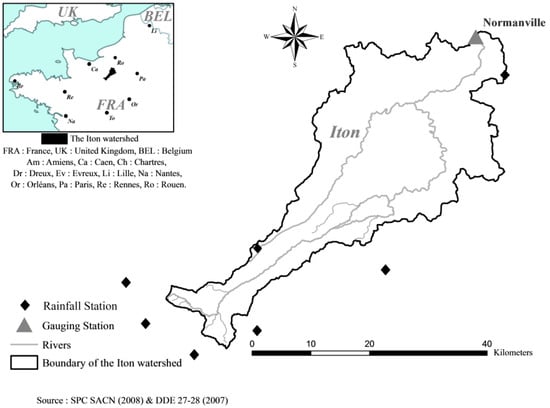
Figure 2.
The Iton watershed.
The Iton watershed rises in the Perche heights and has a drainage area of 1.200 km2 (1038 km2 to Normanville, the last hydrometric station). Generally, it is characterized by a significant evolution of the valley width with elongated deeper valleys upstream and less deep precipitous valleys downstream. This evolution proves the rise of the hydrological behavior of the watershed in the downstream Iton sector especially with contributions from the hydrogeological karst network at Sec-Iton. Indeed, the basin geology is mainly constituted by flint chalk strata with clay passages, limestone with cracks, and significant fracturing [21,22]. These strata, fossilized by impermeable formations based on silt (such as clayey limestone), appear at the plateau, on slopes, and in the bottom of the valleys [23]. This condition has given rise to a complex knowledge of the hydrogeology in the Iton watershed. This hydrogeology directly influences hydrological processes by regulating surface runoff through infiltration rates, disrupting stream flow via the aquifer–river interconnection in quaternary formations at the valley bottoms, and facilitating flow exchanges with neighboring rivers through chalky slicks and karstic networks. In Iton, these underground pathways are highly developed, further enhancing subsurface water movement. In the valley bottoms, these karstic phenomena are essentially reflected by the total or partial disappearance of the surface flow in favor of chalky slick (like Sec-Iton river). The importance of karstic networks in the Iton surface hydrology is estimated from the high capacity of the sources and resurgences like Bonneville-sur-Iton (1250 l.s−1) and Gaudreville-la-Rivière/Glisolles (1050 l.s−1) downstream of Sec-Iton. However, the exact volumes of karst flows remain poorly identified due to the uncertain activity of the karstic networks, clay clogging, and the lack of continuous hydrogeological monitoring. The incorrectly identified influence of karstic networks was however proved in extreme hydrological events (flood and low water).
The flood forecast service of Haute-Normandie (SPC76) and Météo-France services provided the hydrometric data used in this study. ANNs are applied first to the calibration and second to the use of a flood prediction model. It uses time series of mean rainfall P and flow rate Q for the river Iton’s watershed. River Iton’s flooding risk is poorly identified, especially given the presence of karst networks that disturb surficial and subterraneous flows. For this reason, Normanville station’s hydrometric records lack (1) information about red levels of alert and (2) a minimum number of floods associated with an orange level of alert. Table 1 presents rainfall events recorded at Normanville station in the years 1994, 1995, 1998, 2000, 2001, and 2002.

Table 1.
Database used for ANN model.
To reduce overfitting, the database used for calibration is randomly split into three distinct parts (i) The training set is used to recognize the system dynamics. It is the most important (70%). (ii) The test set (20%) is used to avoid over-training by verifying and testing the evolution of the two training errors. (iii) The validation set is performed after the training phase is completed and the most powerful model interconnection weights are recorded. This part of the data (10%) accounts for the confirmation of the performance of the ANN model calculated. The randomness of the division of the database enables an acceptable representation of the different events during the three phases of the ANN model’s calibration.
5. Results and Discussion
This part presents the results for the different steps of the modeling: a computing phase performed in order to determine the ANN’s optimal architecture, the model’s calibration, and the model’s validation.
5.1. ANN Architecture
As previously stated, the ANN is made of an input layer, a single hidden layer, and an output layer with activation functions (logistic sigmoid type) at the level of the artificial neurons. The determination of the optimum ANN architecture is conducted through an experimental phase (trial–error), through which different input combinations (rainfall and flow rate) are tested and assessed. This step was preceded by the use of cross-correlation between Q(t + 6 h) and the different historic variables of both the flow rate and rainfall. The cross-correlation results indicate that the explanatory variables are the 22 antecedent times of rainfall (from P(t) to P(t − 21 h)) and the 30 antecedent times of flow rate (from Q(t) to Q(t − 29 h)).
The execution of the different ANN combinations, with Equation (9), leads to a meaningful choice of the input variables of the prediction model. The output is the flow rate observed at the first term of the flood prediction at t + 6 h. The inputs are different combinations of both rainfall and flow rate variables.
where n is between 1 and 21, and m is between 1 and 29.
The assessment of the ANN modeling starts using the results of the validation phase. Table 2 shows the different results assessed following numerical performance criteria (NASH, MARE, and CP). For a 6 h prediction, these criteria indicate satisfying, eligible results for all the combinations: a NASH superior to 0.99, a MARE inferior to 2.60%, and CP superior to 0.9. However, it is noted that the NASH criterion does not show a large variation for t + 6 h prediction and, therefore, is not very discriminant for the classification of different ANN models. This leads to the comparison of the remaining criteria (MARE and CP). The ANN model with the highest level of performance comprises 13 input variables for rainfall and 30 input variables for the flow rate (Table 2). These variables are the final ones capable of holding information about future flow rates at the Iton River’s outlet.
Table 2.
Results of the different input scenarios of the ANN model.
Consequently, the optimum ANN architecture determined for the flood prediction up to t + 48 h contains 13 inputs for rainfall (from P(t) to P(t − 12) and 30 inputs for the flow rate (from Q(t) to Q(t − 29)) in the input layer, 23 neurons in the hidden layer, and a single neuron in the output layer, with the sigmoid function as the activation function for the two last layers (Figure 3). The mathematical relationship of the ANN modeling is as follows:
where Q(t + t0) is the flow rate to forecast at t0.
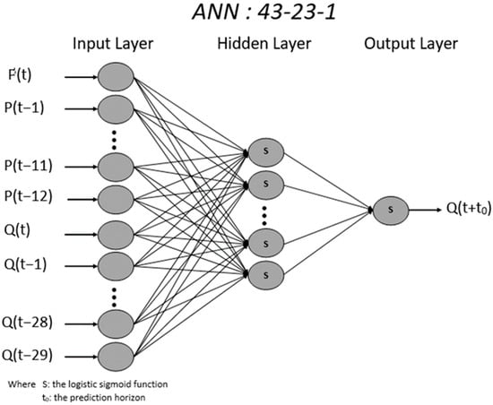
Figure 3.
Optimum architecture of the ANN model predicting floods at Normanville station.
5.2. Application of ANN Model: Flood Prediction
The determination of the optimum architecture of the model for Normanville station allows us to calibrate the ANN model that aims at predicting future flow rates (with a PH between 6 h and 48 h) and assess the model’s performance. This architecture (ANN: 43-23-1) is applied to all the flood prediction models (t + 6 h, t + 12 h, t + 24 h, and t + 48 h) with the database previously used. Again, modeling includes three phases: training, test, and validation.
The calibration of the ANN models used for prediction was conducted in such a way that the difference between the training and test errors converges. The weights of the inter-layer connections are thus produced. The quality of the calibration is assessed thanks to performance criteria (described above), and the results are presented in Table 3. The criteria are calculated by first considering the future flow rate obtained from the three calibration phases of the ANN models for the different PHs.
Table 3.
Performance criteria for the various modeling phases concerning prediction time.
The numerical assessment of the model, through the aforementioned performance criteria, indicates high quality in the estimates of future discharge flows (t + 6 h, t + 12 h, t + 24 h, and t + 48 h). This shows that these models are effective, as they produce flow rates close to reality (MARE (validation t + 6 h) = 3.59%). CP values point to non-naïve predictions between t + 6 h and t + 48 h, with values close to 1. The ANN prediction decreases as the PH increases. This indicates an increase in the error produced and therefore a loss in the computation accuracy. This loss in accuracy remains acceptable, as the errors are low (MARE (validation t + 48 h) = 8.39%), and the predictive capability is strong (CP (validation t + 48) = 0.89).
A comparison of the evolution of each numerical criterion during the three phases of calibration is shown in Figure 4. The MARE and NASH criteria evolve similarly (Figure 4a,c). This evolution indicates a pseudo-stability of the general calculation performed by the ANN while passing from one phase to another. In contrast, for each PH, the CP values during the training phase are lower than those in the test and validation phases (Figure 4b). This discrepancy highlights the negative impact of data quality, as inconsistencies in the collected data sometimes diverge from the system’s overall response. However, the model’s prediction is enhanced after estimating the different inter-neuron weights during the training phase. In fact, the convergence between the test and training errors makes the estimated weights closer to reality and shows an improvement in the prediction during the test phase (consequently during the validation phase too). This improvement presents a better understanding of the hydrological response of the river Iton to the different input parameters after completing the model’s calibration. As the prediction time increases, the MARE criterion rises, while NASH and CP decline across the training test and validation phases. Consequently, the model loses accuracy as the prediction time increases. This loss in accuracy remains satisfying, as CP equals 0.89 during the validation phase at t + 48 h.
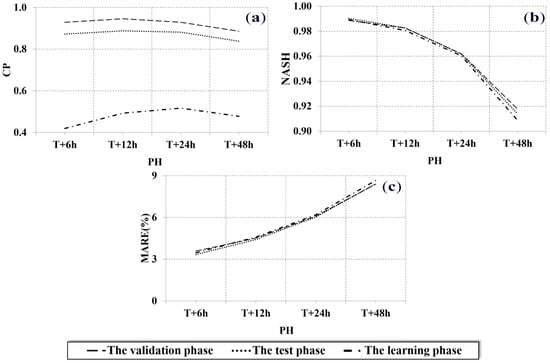
Figure 4.
Comparison of performance criteria per phase of the ANN modeling between PH t + 6 h and t + 48—(a) NASH; (b) CP; and (c) MARE.
The prediction results of the flow rates at Normanville station have been graphically assessed. Figure 5 shows a comparison between the observed and calculated flow rates for different PHs during the validation phase. The point clouds, representing the calculated flow rates against the observed ones, closely align with the one-to-one function (X = Y) across the different PHs. This indicates a good correlation between the observed and calculated data, especially for high values of flow rate. These good correlations are reflected by the similarity of both observed and calculated flood hydrographs. This suggests accurate predictions with a slight temporal shift in shapes and peaks. A dispersion of the point cloud around the X = Y curve is noted when the PH increases. This dispersion implies a decrease in the correlation coefficient. The magnitude of the point cloud’s dispersion depends on the value of the flow rate planned. This is important when the flow rate is small and decreases as the flow rate increases (Figure 5). The graphical analysis is upheld by the analysis of the prediction results according to the alert level (Table 4). This shows a higher convergence of the ANN model when the flow rate is increased (when the alert level increases). Between t + 6 h and t + 18 h, less ANN modeling errors are recorded when the alert shifts from green to yellow and orange and red. From t + 24 h onward, predictions at the orange and red alert levels exhibit higher errors than those at the green and yellow levels. These errors can be explained by the limited quantity of information (contained in the database) concerning extreme floods (orange and red levels of alert). However, these errors remain acceptable (MARE (t + 48 h) = 12.29) and indicate a good quality of prediction up to t + 48 h.

Figure 5.
Comparison between observed and calculated flow rates by the ANN model (events between January and April 2001)—(a) t + 6 h; (b) t + 12 h; (c) t + 24 h; and (d) t + 48 h. CF: calculated flow rate; OF: observed flow rate.
Table 4.
MARE criterion according to the alert level.
The flood prediction ANN model has a tendency to predict flood development and an extreme flow rate with a high correlation; oppositely, the quality decreases for small flow rates.
6. Conclusions
This paper has clearly proven the interest and potential application of using an ANN model to forecast the complex rainfall–runoff relationship of the Iton watershed.
The best ANN architecture tested has three layers (43-23-1 neurons) and uses a sigmoid-type function. This model provides excellent results considering its quality assessment. The quality assessment of MARE, NASH, and CP criteria across the training, test, and validation phases confirms a strong correlation between the in situ hydrological measurements and the model predictions. The precision is still acceptable at t + 48 h, as the errors remain low (MARE (validation t + 48 h) = 8.39%), and the prediction accuracy is high (CP (validation t + 48) = 0.89).
This accuracy is more than sufficient for flood warning applications. Moreover, the calculation time is very short (i.e., a few seconds), which enables a near-real-time update of the flood peak forecast. This type of model allows public services in charge of flood risk protection to warn people and municipalities with a reliable horizon of 48 h. This delay allows for the implementation of mitigation solutions, whereas the nonlinear relationship of rainfall–runoff is a limiting factor in the prediction of hydrological risks.
Author Contributions
Conceptualization, M.-T.A.; Methodology, O.K.; Software, O.K.; Formal analysis, R.A. and M.-T.A.; Investigation, R.A.; Writing—review & editing, A.B. All authors have read and agreed to the published version of the manuscript.
Funding
This research received no external funding.
Data Availability Statement
The data presented in this study are available on request from the corresponding author.
Conflicts of Interest
The authors declare no conflict of interest.
References
- Khorchani, M.; Blanpain, O. Development of a Discharge Equation for Side Weirs Using Artificial Neural Networks. J. Hydroinform. 2005, 7, 31–39. [Google Scholar] [CrossRef][Green Version]
- Coulibaly, P.; Anctil, F.; Bobée, B. Daily Reservoir Inflow Forecasting Using Artificial Neural Networks with Stopped Training Approach. J. Hydrol. 2000, 230, 244–257. [Google Scholar] [CrossRef]
- Lallahem, S.; Mania, J. A Nonlinear Rainfall-Runoff Model Using Neural Network Technique: Example in Fractured Porous Media. Math. Comput. Model. 2003, 37, 1047–1061. [Google Scholar] [CrossRef]
- Riad, S. Typologie et Analyse Hydrologique Des Eaux Superficielles à Partir de Quelques Bassins Versants Représentatifs du Maroc. Ph.D. Thesis, Université de Lille, Lille, France, 2003. Available online: https://theses.fr/2003LIL10122 (accessed on 17 March 2025).
- Toukourou, M. Application de l’apprentissage Artificiel à La Prévision Des Crues Éclair. Ph.D. Thesis, École Nationale Supérieure des Mines de Paris, Paris, France, 2009. Available online: https://theses.fr/2009ENMP1669 (accessed on 17 March 2025).
- ASCE Task Committee on Application of Artificial Neural Networks in Hydrology. Artificial Neural Networks in Hydrology. II: Hydrologic Applications. J. Hydrol. Eng. 2000, 5, 124–137. [Google Scholar] [CrossRef]
- Thiria, S.; Lechevallier, Y.; Gascuel, O. Statistique et Méthodes Neuronales; Sciences sup; Dunod: Malakoff, France, 1997; ISBN 2-10-003544-4. [Google Scholar]
- Taud, H.; Mas, J.F. Multilayer Perceptron (MLP). In Geomatic Approaches for Modeling Land Change Scenarios; Camacho Olmedo, M.T., Paegelow, M., Mas, J.-F., Escobar, F., Eds.; Springer International Publishing: Cham, Switzerland, 2018; pp. 451–455. ISBN 978-3-319-60801-3. [Google Scholar]
- Lippmann, R. An Introduction to Computing with Neural Nets. IEEE ASSP Mag. 1987, 4, 4–22. [Google Scholar] [CrossRef]
- Hornik, K.; Stinchcombe, M.; White, H. Multilayer Feedforward Networks Are Universal Approximators. Neural Netw. 1989, 2, 359–366. [Google Scholar] [CrossRef]
- Najjar, Y.M.; Basheer, I.A.; Hajmeer, M.N. Computational Neural Networks for Predictive Microbiology: I. Methodology. Int. J. Food Microbiol. 1997, 34, 27–49. [Google Scholar] [CrossRef] [PubMed]
- Lek, S.; Dimopoulos, I.; Derraz, M.; El Ghachtoul, Y. Modélisation de la relation pluie-débit à l’aide des réseaux de neurones artificiels. Rev. Sci. L’eau J. Water Sci. 1996, 9, 319–331. [Google Scholar] [CrossRef][Green Version]
- Boleratz, B.L.; Oscar, T.P. Use of ComBase Data to Develop an Artificial Neural Network Model for Nonthermal Inactivation of in Milk and Beef and Evaluation of Model Performance and Data Completeness Using the Acceptable Prediction Zones Method. J. Food Saf. 2022, 42, e12983. [Google Scholar] [CrossRef]
- Funahashi, K.-I. On the Approximate Realization of Continuous Mappings by Neural Networks. Neural Netw. 1989, 2, 183–192. [Google Scholar] [CrossRef]
- Chokmani, K.; Ouarda, T.B.M.J.; Hamilton, S.; Ghedira, M.H.; Gingras, H. Comparison of Ice-Affected Streamflow Estimates Computed Using Artificial Neural Networks and Multiple Regression Techniques. J. Hydrol. 2008, 349, 383–396. [Google Scholar] [CrossRef]
- Bowden, G.J.; Dandy, G.C.; Maier, H.R. Input Determination for Neural Network Models in Water Resources Applications. Part 1—Background and Methodology. J. Hydrol. 2005, 301, 75–92. [Google Scholar] [CrossRef]
- Nash, J.E.; Sutcliffe, J.V. River Flow Forecasting through Conceptual Models Part I—A Discussion of Principles. J. Hydrol. 1970, 10, 282–290. [Google Scholar] [CrossRef]
- Organisation Meteorologique Mondiale. Intercomparison of Conceptual Models Used in Operational Hydrological Forescasting—OMM (WMO) N° 429; Secretariat of the World Meteorological Organization: Geneva, Switzerland, 1975. [Google Scholar]
- Siou, L.K.A. Modélisation Des Crues de Bassins Karstiques Par Réseaux de Neurones. Cas Du Bassin Du Lez (Hérault); Université Montpellier II—Sciences et Techniques du Languedoc: Montpellier, France, 2011; Available online: https://theses.hal.science/tel-00649103 (accessed on 17 March 2025).
- Masson, E.; Kharroubi, O.; Blanpain, O.; Lallahem, S. Chroniques Hydrométriques et Prévision Des Crues Par Modélisation Hydrologique à Base de Réseau de Neurones Artificiels (RNA) Dans Le Bassin-Versant de l’Eure. Rev. Nord. Hors Série 2011, 16, 35–45. [Google Scholar]
- Moguedet, G.; Marchand, Y.; Masson, V.; Papin, H.; Vauthier, S.; Charnet, F.; Le Moine, B. Notice Explicative, Carte Géol. France (1/50 000), Feuille La Loupe (253); BRGM: Orléans, France, 2000; 102p. [Google Scholar]
- Ménillet, F. Avec La Collaboration Des Différents Services Du B.R.G.M. Orléans et de R.VERMEIRE. (1971)—Notice Explicative, Carte Géol. France (1/50000), Feuille Chartres (255); Bureau de Recherches Géologiques et Minières: Orléans, France, 1971; 35p. [Google Scholar]
- Kuntz, G.; Dewolf, Y.; Frileux, P.-N.; Monciardini, C.; De La Quérière, P.; Verron, G. Notice Explicative, Carte Géol. France (1/50000), Feuille Breteuil-Sur-Iton (179); BRGM: Orléans, France, 1982; 38p. [Google Scholar]
Disclaimer/Publisher’s Note: The statements, opinions and data contained in all publications are solely those of the individual author(s) and contributor(s) and not of MDPI and/or the editor(s). MDPI and/or the editor(s) disclaim responsibility for any injury to people or property resulting from any ideas, methods, instructions or products referred to in the content. |
© 2025 by the authors. Licensee MDPI, Basel, Switzerland. This article is an open access article distributed under the terms and conditions of the Creative Commons Attribution (CC BY) license (https://creativecommons.org/licenses/by/4.0/).