A Simulation-Optimization Approach of Geothermal Well-Doublet Placement in North China Using Back Propagation Neural Network and Genetic Algorithm

Abstract

The well-doublet production model has far-reaching implications for the sustainable utilization of geothermal resources. The position of the injection well in the geothermal production process is closely connected to the emergence of thermal breakthroughs and the production lifespan. Thus, it is necessary to optimize the well placement. However, traditional simulation and optimization approaches require a long time and have a high computing burden. In this paper, a surrogate model based on the back propagation neural network (BPNN) is trained to improve the drawbacks of previous approaches, and it is combined with the genetic algorithm (GA) to develop a simulation-optimization approach to find the optimal well placement of a well-doublet geothermal production system. To guarantee that the training data have appropriate physical significance, the TOUGH2 program is used for the hydro–thermal model development of the geothermal reservoir of the Minghuazhen Formation in Tianjin, China. A sensitivity analysis is used to select the series of samples used for training, which includes temperature and pressure variation, heat extraction rate (Wh), and economic cost. The results reveal that the surrogate model has excellent prediction accuracy and efficiency for physical processes, and the genetic algorithm optimization outcomes are consistent with predictions, which is of practical importance.

1. Introduction

Energy plays a pivotal role in driving the development of economic and social systems. In the context of energy conservation, the accelerated construction of modern energy systems and the promotion of renewable energy development are critical for both economic growth and carbon emission reduction. Geothermal energy, as an alternative and renewable energy source, has gained prominence over other forms of clean energy due to its widespread distribution, safety, low operating costs, and suitability for heating and power generation [1,2].

Geothermal resources are mainly concentrated in tectonically active regions such as the Pacific Ring of Fire and the Mediterranean–Himalayan geothermal belt. Among these, sandstone reservoirs are a key medium for low- to medium-temperature geothermal systems, accounting for approximately 40–60% of geothermal resources in sedimentary basins. These resources have considerable utilization potential [3]. In China, sandstone geothermal resources offer significant advantages, particularly in areas such as the North China Basin, where proven reserves reach 3.2 × 10¹⁸ kJ [4]. The reservoir thickness generally exceeds 1000 m, and the geothermal gradient ranges from 3.5 to 4.5 °C/100 m. Tianjin, a typical representative of this region, ranks highly in China for both the quality and scale of its sandstone geothermal resources [5]. When compared to similar sedimentary basins internationally, its resource parameters are also regarded as being of high quality.

In Tianjin, geothermal resources are abundant, covering an area of 8700 km² [6]. Exploitation of these resources is focused on three major thermal reservoirs: the Minghuazhen Formation, Guantao Formation, and Wumishan Formation [7]. These reservoirs are generally highly permeable, facilitating the effective extraction of geothermal energy. Since the 1970s, Tianjin has developed a comprehensive approach to geothermal energy utilization, which includes heating, bathing, aquaculture, and agriculture [8].

The large-scale production of geothermal resources in the Tianjin area has led to issues such as excessive groundwater extraction and ground subsidence. Well-doublet production can help mitigate these problems by reinjecting the tail thermal water into the reservoir. However, improper well placement can result in thermal breakthrough, where low-temperature tailwater moves quickly to the production well, reducing the water temperature. Therefore, it is essential to optimize well placement. Akin et al. [9] highlighted the advantages of well-doublet systems over single wells in maintaining reservoir pressure and reducing waste heat pollution. Compared to field drilling tests and laboratory experiments, numerical simulation offers significant advantages for well optimization due to its low cost, convenience, and high efficiency.

Numerical simulation is an effective and cost-efficient method for evaluating the productivity of geothermal well-doublet systems. These models help assess energy efficiency, predict geothermal development, and monitor temperature evolution in both the production and injection wells, which is essential for optimizing well placement. Recent studies have applied numerical simulations to geothermal reservoirs. Ding et al. [10] determined several crucial factors that affect thermal productivity via the numerical simulation of a well-doublet. These factors are natural geological parameters, such as reservoir permeability [11,12], temperature [13,14], and pressure [11,15], and operating condition parameters, such as well distance [11,15], injection angle [10,16], and injection pressure [13,15]. Furthermore, Liu et al. [17] investigated the productivity mode of heterogeneous porous geothermal reservoirs by constructing a hydro–thermal–mechanical coupling model for well-doublet production. The result shows that a high permeability fracture channel between wells runs through the production well and injection well, leading to thermal breakthroughs. In addition, Zhou et al. [18] found that the flow direction and velocity of groundwater would directly affect the evolution of the groundwater temperature field, and then affect the occurrence time of the thermal breakthrough effect when studying the factors affecting the efficiency of the multi-well groundwater heat pump system (GWHP). Therefore, during well placement optimization, analysis through numerical simulation models can identify the key parameters that impact well productivity. Additionally, these parameters can be specifically focused on and adjusted.

To optimize the productivity of the well-doublet system and minimize negative impacts on the reservoir, traditional well placement optimization methods primarily involve sensitivity analysis to identify key factors affecting temperature and pressure evolution, such as flow field state, reservoir structure, well spacing, and production/injection flow rates [19]. Optimization principles are usually established by setting threshold values for state variables like bottom pressure and wellhead temperature. For example, Schulte et al. [20] used strategies such as “minimum reservoir pressure difference” and “maximum productivity” to optimize well placement, delaying thermal breakthrough and reducing water loss. The critical factor is the relative position between the production well and injection well, and optimization is achieved by adjusting well site parameters accordingly. Recently, new methods have advanced well placement optimization. Zhang et al. [21] introduced the “One Factor at a Time (OFAT)” method for optimizing well placement. Blank et al. [22] proposed an optimization framework based on finite element analysis and gradient-free optimization, studying the impact of multi-well placement on the long-term performance of geothermal reservoirs. Additionally, Zhang et al. [23] developed the single-well-injection-test (SWIT) optimization method, which has been applied in large-scale thermal field development.

However, traditional well placement optimization requires the use of a large number of physical simulation models, such as water flow-heat transfer models, which result in substantial computational load and long simulation times. Additionally, the process struggles with poor portability under varying conditions [24]. However, artificial intelligence (AI) methods provide an alternative by creating surrogate models derived from the extensive training of simulation results. These AI models can quickly determine threshold values within a given optimization framework based on engineering operation parameters. The use of AI significantly enhances the efficiency of well placement optimization, and it has garnered increasing attention due to its potential to streamline the optimization process [25].

AI optimization algorithms are gaining popularity across various fields because of their low cost, strong adaptability, and high degree of automation. In geothermal production, AI optimization algorithms can substantially reduce the time required for well placement optimization [26]. Several scholars have successfully combined AI algorithms, such as genetic algorithms [27,28], cat swarm algorithms [29], and bee swarm algorithms [30], with geothermal reservoir numerical simulations to optimize the placement of multi-well or well-doublet systems. These efforts have led to notable progress. However, traditional AI optimization algorithms often rely on a large number of site parameters and mainly focus on the physical properties of the geothermal reservoir [28], which may fail to account for the actual physical processes involved. On the other hand, machine learning-based optimization algorithms offer significant improvements in operational time efficiency, often saving several orders of magnitude in comparison to traditional methods [25]. For instance, Grant et al. [31] applied a data-driven thermodynamic approach, creating geothermal operational optimization with machine learning (GOOML) that provides high prediction accuracy using machine learning techniques. Additionally, Gudala et al. [32] enhanced the traditional simulation model by integrating it with an AI model named machine learning-response surface model-autoregressive integrated moving average (ML-RSM-ARIMA), offering a novel approach to accurate prediction and well location optimization in geothermal systems.

In addition to more advanced optimization algorithms, constructing surrogate models for the numerical simulation process is also a key factor in improving the speed of well placement optimization. These surrogate models, derived from the results of extensive numerical simulations, can significantly reduce the computational cost and time required for optimization, making it possible to quickly evaluate different well placement configurations. Among various machine learning methods, the back propagation neural network (BPNN) stands out as a powerful tool for energy-related applications, such as natural gas load forecasting [33] and coal gasification output prediction [34]. BPNN excels in solving multi-dimensional nonlinear problems and offers a faster training speed and high model regression accuracy [35]. Despite its effectiveness, BPNN has been rarely applied to geothermal well placement optimization. Its ability to construct surrogate models makes it an ideal candidate for improving well placement optimization, providing both high accuracy and fewer iterations compared to other AI methods. Given these advantages, further research is needed to explore the full potential of BPNN in geothermal well placement optimization.

The main innovations of this study in geothermal well-doublet placement optimization are summarized as follows: (1) A new well placement optimization principle is proposed by introducing heat extraction efficiency and economic evaluation parameters, which are based on the physical states of reservoir temperature and pressure during the production process. (2) In constructing the surrogate model for well-doublet production, a sensitivity analysis is performed on well placement parameters and engineering operational parameters that may lead to changes in the reservoir’s temperature and pressure state. The causal relationship between input and output, as envisioned in the machine learning model, is established, thus determining the inputs for the surrogate model. (3) A well-doublet geothermal production simulation-optimization model based on the BPNN and GA algorithm is proposed. The BPNN algorithm is used to construct a surrogate model for the hydro–thermal model during the production process, and the surrogate model is invoked in the GA optimization process for well placement. This approach reduces the high computational burden caused by the previous use of numerical simulation models and improves the efficiency of well placement optimization.

2. Study Area

Tianjin is located in North China, faces the Bohai Sea to the east and belongs to the Haihe River basin. Additionally, Tianjin has by far the largest medium–low temperature geothermal field in China, with the characteristics of a shallow buried depth and good thermal physical properties.

The study area of this work is the Panzhuang Uplift area located in the northeast of Tianjin (Figure 1), which belongs to the Cangxian Uplift area. The Mesozoic Yanshan movement and the Cenozoic Himalayan movement caused numerous complex fault zones in the area, which serve as effective channels for geothermal water’s heat and water conduction. In addition, the Quaternary caprock develops well in the study area, which provides a good thermal insulation condition for the storage of geothermal resources. The simulated geothermal reservoir is the Minghuazhen Formation of the Neogene System in the study area. The Minghuazhen Formation is distributed across the whole study area with an average thickness of more than 500 m, which belongs to a porous geothermal reservoir. It is divided into two sections in the study area. The lithology of the upper section is mainly composed of silty sand and fine sandstone with mudstone, the roof buried depth is 400~500 m, the porosity is 27.97~39.5%, and the effluent temperature is 45~50 °C. The lower lithology is mainly mudstone, the roof buried depth is 800~900 m, the porosity is 21.3~30.5%, and the effluent temperature is 65~75 °C [36].

The reservoir of the Minghuazhen Formation in the study area has been exploited on a large scale because of the characteristics of a shallow buried depth, easy exploitation, and low exploitation cost. The over-exploitation of geothermal resources leads to a decrease in groundwater level and reservoir pressure, which increases operational costs and might potentially lead to hydrogeological and environmental issues. In recent years, Tianjin has effectively ensured the sustainable development of middle and deep geothermal resources. This has been achieved by restricting the exploitation of sandstone geothermal reservoirs. Additionally, the region has largely maintained the stability of the geothermal reservoir’s water level by reinjecting geothermal tailwater back into the exploited reservoir. Although, during the reinjection process, the lower solubility of high-concentration ions, such as calcium and magnesium in geothermal water, or chemical reactions, may form reinjection structures that hinder the reinjection process. However, to date, the geothermal-doublet system remains the main method for exploiting medium and low-temperature geothermal resources.

3. Methodology

3.1. Numerical Simulation Algorithm

The numerical simulation is done by the TOUGH2 program (TOUGHREACT Version 2.0 EOS1), which can realize the non-isothermal numerical simulation of multi-component and multiphase fluids in multi-dimensional porous fractured media [37]. In this study, the TOUGH2 program is used to construct a hydro-thermal coupling model for the geothermal development of well-doublets. The model is based on the thermophysical parameters of the geothermal reservoir of the Minghuazhen Formation in the Panzhuang Uplift structural area of Tianjin. And it is applied to predict the pressure and temperature evolution of the study thermal reservoir in 50 years.

(1)

Model setup

(a)

Assumptions

The aquifer is homogeneous, horizontal, equal thickness, and isotropic.

The pores of the rock are full of fluid and all of them are water, which conforms to Darcy’s law of fluid and does not occur in a phase transition.

The heat transfer mode between fluid and rock skeleton consists of convection and conduction.

(b)

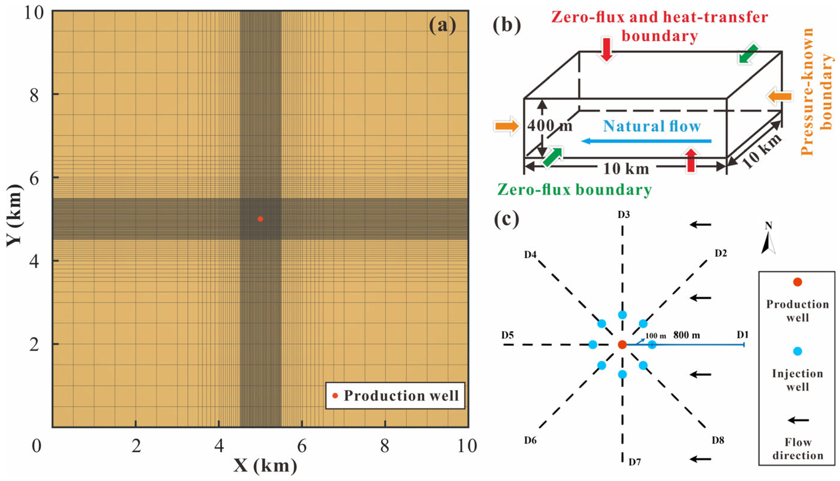
Conception model

The site conceptual model of the target reservoir constructed in this study is shown in Figure 2a. The lengths of the model in the X, Y, and Z directions are 10 km, 10 km, and 400 m, respectively. The geometric center of the X-Y plane is taken as the location of the production well (ignoring the well diameter). The site is spatially discretized according to the principle of ‘far sparse and close density’, relative to the production well [38]. The discrete scale is transferred from 500 m at the far-well area to 10 m at the near-well area in the X and Y direction, and the monolayer grid discretization is carried out in the Z direction (reservoir thickness 400 m). There are 16,900 discrete units in total.

(c)

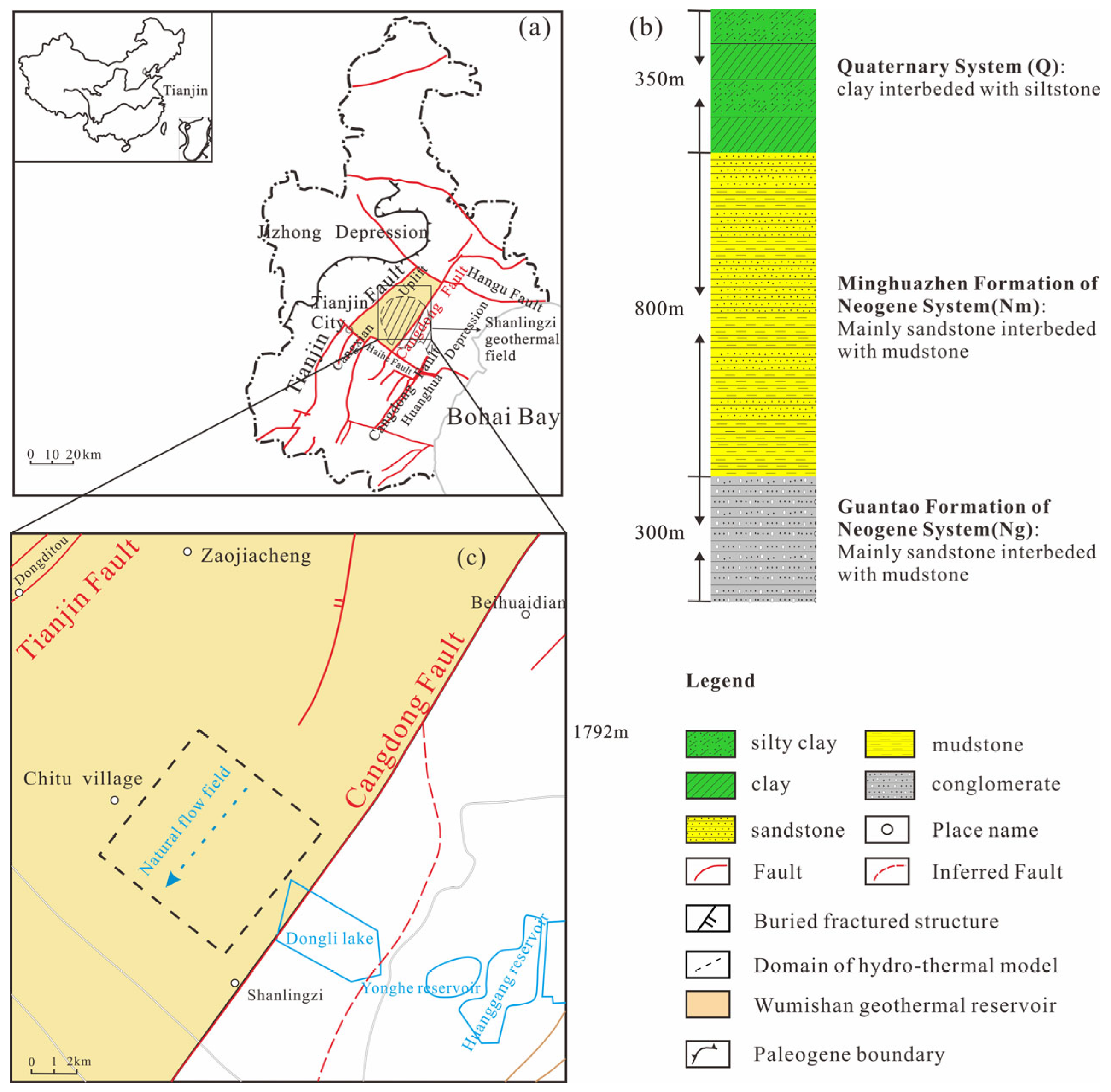
Initial condition

The target reservoir of this study is the Minghuazhen Formation reservoir in the Panzhuang Uplift area of Tianjin. The reasons are as follows: first, the buried depth is shallow, the production cost is low, and it is easy to realize geothermal well-doublet production; second, the data of geotechnical thermophysical parameters are abundant after years of exploitation and research. Based on previous site tests and numerical simulations [36], the main hydrogeological and thermophysical parameters of the Minghuazhen Formation of Neogene System in the study area are shown in

Table 1. Numerical simulation parameters of conceptual model.

Parameters	Values	Unit
Aquifer buried depth	1000	m
Aquifer hydraulic slope	0.001532
Aquifer thickness	400	m
Injection temperature	30.00	°C
Permeability	3.385 × 10−13	m2
Porosity	0.25
Skeleton density	2600	kg/(m3)
Specific heat of rock skeleton	958	J/(kg·K)
Thermal conductivity of rock skeleton	2.5	W/(m·K)
Thermal reservoir temperature	45.58	°C

.

The well-doublet geothermal production system is mainly used for building heating in winter. The heating period starts in mid-November each year and lasts until mid-March of the following year.

(d)

Boundary condition

The reservoir of the Minghuazhen Formation in the study area is a confined aquifer, and the heat transfer between the target reservoir and the surrounding rock is calculated by the semi-analytical solution to improve the calculation efficiency.

The natural groundwater flows from northeast to southwest, the corresponding lateral boundaries (X= 10 km and X = 0 m) are set as constant pressure, and because the range of the numerical simulation area is large enough, the production and injection well cannot cause the change in temperature and pressure at the boundary of the target reservoir. The boundaries (Y = 10 km and Y = 0 m) along the northwest to southeast direction are considered impermeable, resulting in no groundwater flow across them. The boundary conditions of this study area are shown in Figure 2b.

(2)

Well placement scheme

According to the site conceptual model, the 2D coordinate of the production well is (5000, 5000). The production flow rate varies from 40 m³/h to 220 m³/h. The placement schemes of the injection well are shown in Figure 2c. The directions are set at an interval of 45° and the numbers are D1~D8. The well placement is set at an interval of 100 m in all directions, with a total of 64 placements. The 2D coordinate ranges of (5000 ± 800, 5000 ± 800). The injection well will recharge 100% of the thermal tailwater.

3.2. Economic Analysis Method

In order to optimize the well-doublet production cost of the geothermal reservoir according to the social and economic development, it is necessary to make an economic analysis of the total operation cost. The cost of the well-doublet production system ($C$) is related to many factors, but it can be generalized as the change in reservoir pressure and temperature in the reservoir. Therefore, in the economic cost analysis, an objective Equation (1) [39] is introduced to consider the water level reduction and thermal breakthrough of the production reservoir in the future $N$ years, and depreciated according to the depreciation rate of the study area.

$$C=q·\sum _{i=0}^N{\displaystyle \frac{{\left(\Delta P·pp+{\rho }^l·c^l·\Delta T·pr·\eta \right)}_t}{{\left(1+r\right)}^t}}$$

(1)

where $q$ is production or injection flow (kg·m⁻³·s), $N$ is simulated production time (year), $i$ is circulation variable, $\Delta P$ is pressure change at the bottom of production well (Pa), $pp$ is market electricity price (¥), ${\rho }^l$ is geothermal fluid density (kg·m⁻¹), $c^l$ is the specific heat capacity of geothermal fluid (J·kg⁻¹·K⁻¹), $\Delta T$ is temperature change at the bottom of production well (K), $pr$ is market heat price (¥), $\eta$ is heat utilization efficiency, and $r$ is the depreciation rate.

Based on the above objective equation, this study analyzes the total cost of different well-doublet placement schemes of the shallow geothermal reservoir in the Tianjin area in 50 years. The simulation results of the hydro–thermal coupling numerical model are used to calculate the total cost. The analysis result is considered an important index for well placement optimization.

3.3. Back Propagation Neural Network

BPNN is a kind of multi-layer feedforward neural network, which is one of the most widely used neural networks at present. It adopts the learning algorithm of error back propagation and can effectively solve nonlinear problems [40]. The BPNN consists of the input layer, output layer, and hidden layer with different numbers of nodes. The number of nodes in the input layer and output layer depends on the number of input and output arrays, and the number of nodes in the hidden layer needs to be adjusted according to the problem. The specific number of nodes in the hidden layer is determined by the final fitting effect [41].

The main governing equations of BPNN are as follows [41].

(1)

The data output of hidden layer is expressed by Equation (2):

$$y_i=f\left(\sum _j{w}_{ij}{x}_j-{\theta }_i\right)=f\left({net}_i\right)$$

(2)

where $y_i$ is the $i$-th node in the hidden layer, $x_j$ is the $j$-th node in the input layer, $w_{ij}$ is the weight between the $i$-th node of the input layer and $j$-th node of the hidden layer, and ${\theta }_i$ is the i-th threshold value in the hidden layer.

(2)

The data output of output layer is expressed by Equation (3):

$$O_l=f\left(\sum _i{T}_{li}{y}_i-{\theta }_l\right)=f\left({net}_l\right)$$

(3)

where $O_l$ is the $l$-th node in the output layer, $T_{li}$ is the weight between the $l$-th node of input layer and $i$-th node of hidden layer, and ${\theta }_l$ is the $l$-th threshold value in the hidden layer.

(3)

The error calculation function of output node is according to Equation (4):

$$\begin{array}{c}E={\displaystyle \frac{1}{2}}{\displaystyle \sum _l}{\left(t_l-O_l\right)}^2={\displaystyle \frac{1}{2}}{\displaystyle \sum _l}{\left[t_l-f\left({\displaystyle \sum _i}{T}_{li}{y}_i-{\theta }_l\right)\right]}^2\\ ={\displaystyle \frac{1}{2}}{\displaystyle \sum _l}{\left\{t_l-f\left[{\displaystyle \sum _i}{T}_{li}f\left({\displaystyle \sum _j}{w}_{ij}{x}_j-{\theta }_i\right)-{\theta }_l\right]\right\}}^2\end{array}$$

(4)

where $E$ is the error of the output node, and $t_l$ is the expected value of the output node.

In this study, an optimization model of geothermal reservoir well-doublet production is obtained by the BPNN algorithm. The training data for the BPNN are the result of the hydro–thermal coupling model, heat extraction rate analysis, and economic analysis.

4. Results

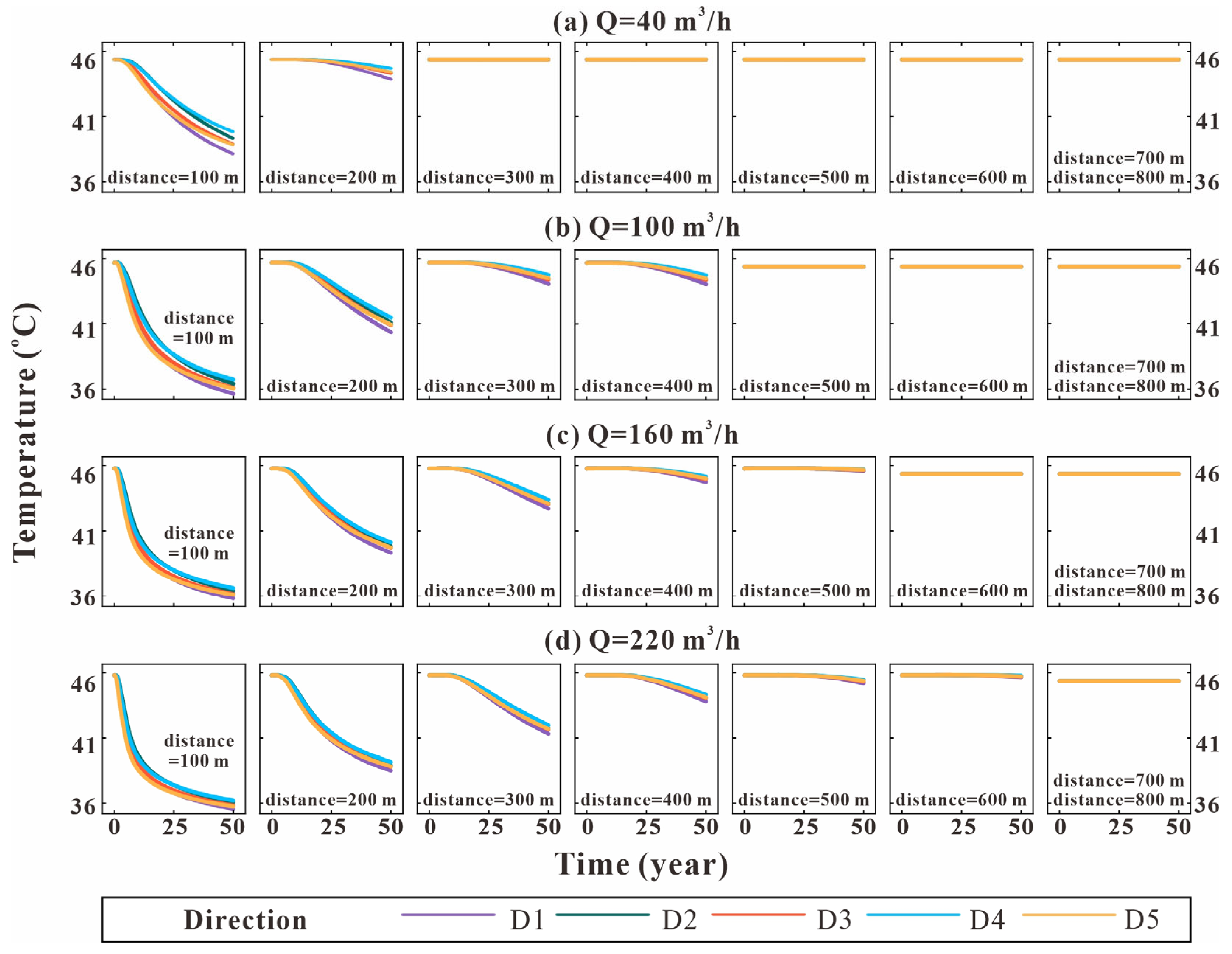
4.1. Temperature

Temperature evolution in production wells is related to well distance. Thermal breakthroughs are more likely to occur with short well distances; however, long well distances can mitigate the influence of thermal breakthroughs. When the well distance is small, the temperature drops in all directions over time. The flow field of low-temperature water injected into the reservoir spreads swiftly. It reaches the production well, causing a continuous decrease in temperature at the bottom of the well. This leads to the thermal breakthrough phenomenon. When the well distance was 300 m (Figure 3a), no thermal breakthrough occurred for the first time in the group with an injection flow rate of 40 m³/h. The injection flow rate influenced the critical well distance of thermal breakthrough. Compared to the modest injection flow rate, a large injection flow rate increases the likelihood of thermal breakthrough phenomena. This occurs after the well-doublet system has operated for the same amount of time. In the groups with injection flow rates of 100 m³/h, 160 m³/h, and 220 m³/h, the critical well distance of thermal breakthrough was 400 m, 500 m, and 600 m (Figure 3b–d), respectively. When the well distance is longer than the critical well distance, the temperature stays steady, and the injection tail water has no influence on the temperature of the production well.

The temperature development process is influenced by the injection angle. With equal well distance, the directions of D4 and D6 showed less temperature change compared to the other directions in each injection flow group. In other words, they are less prone than other injection angle techniques to have thermal breakthroughs.

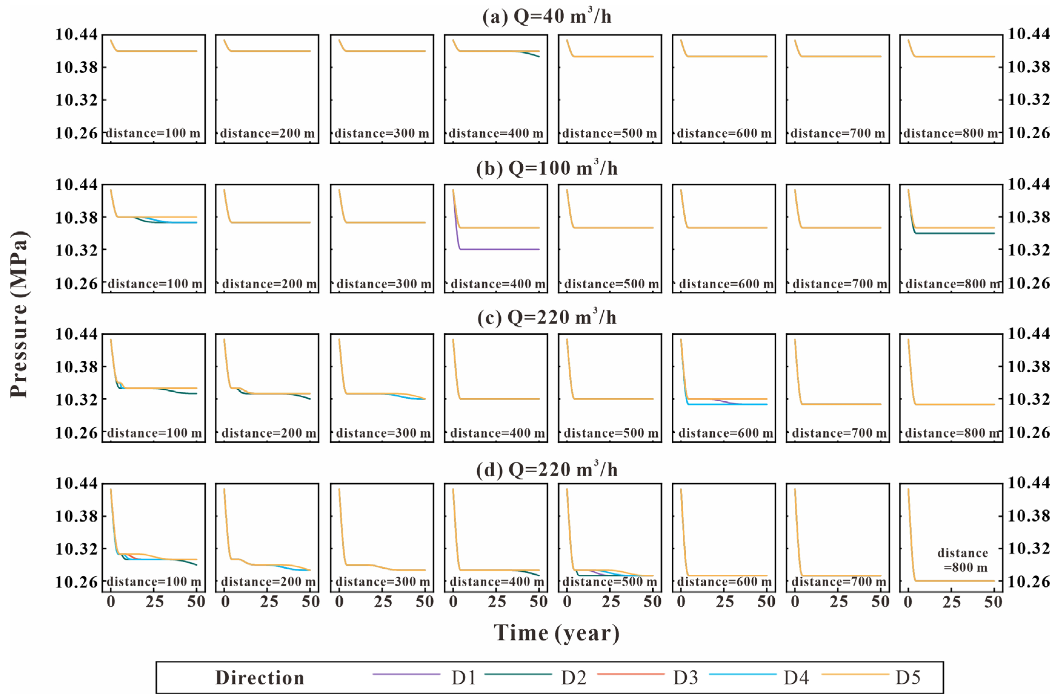
4.2. Pressure

Compared to temperature, pressure varies dramatically at long well distances in each injection flow group. The pressure at the bottom of the production well decreases dramatically in the early stages of system operation. The range of decline expands as the recharge flow and well distance increase. At a 100 m well distance, the minimum pressure increases for each injection flow group were 0.02 MPa, 0.05 MPa, 0.09 MPa, and 0.13 MPa (Figure 4). The variation in the pressure is also different in each direction. Generally, the pressure drops in downstream of the production well are smaller than that in the upstream.

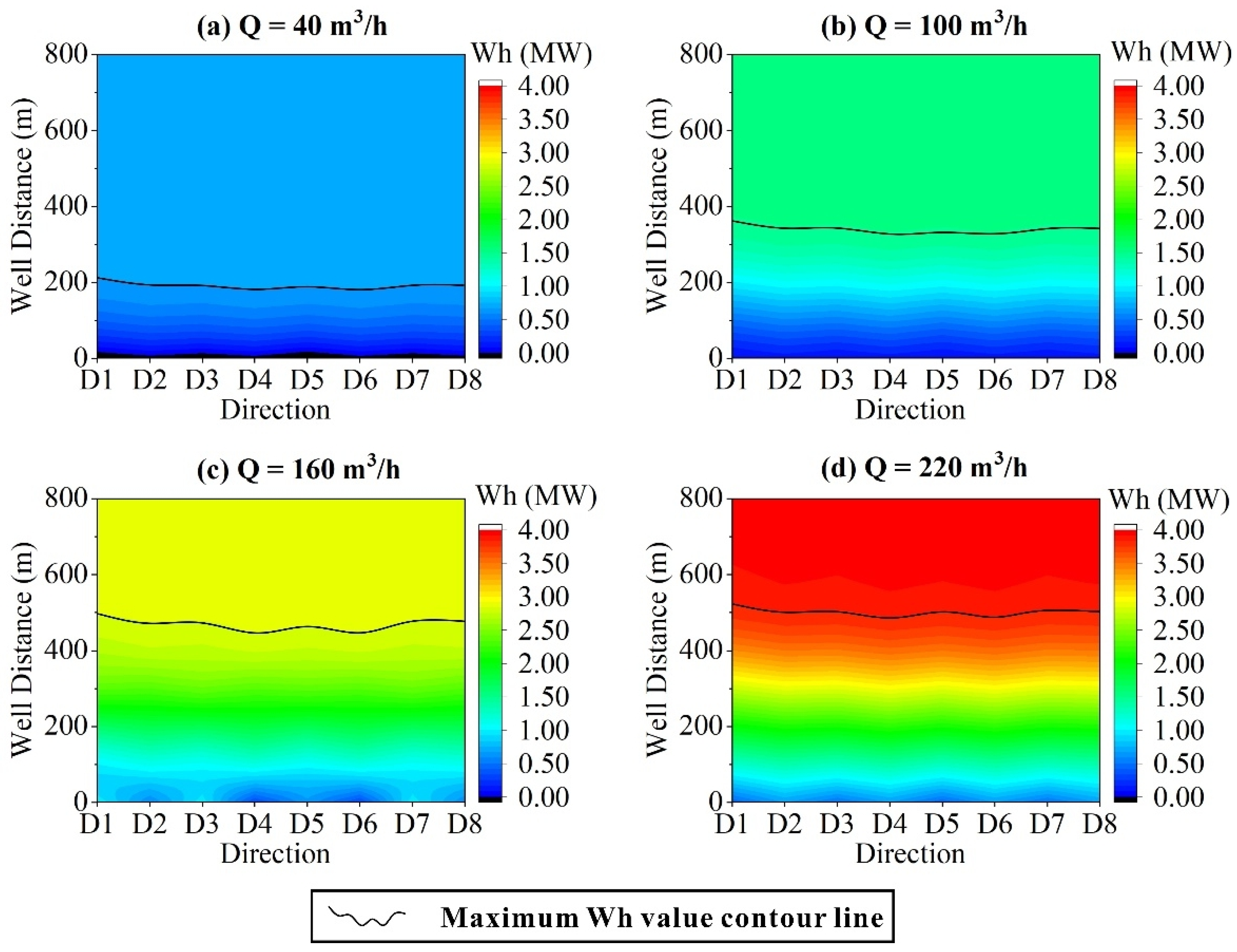
4.3. Heat Extraction Rate

In addition to the changes in temperature and pressure within the reservoir, the thermal extraction efficiency of the well-doublet system and the extra economic costs throughout the production cycle are also considered as outputs of the model. Therefore, before constructing the surrogate model, it is necessary to first calculate the relevant parameters. Furthermore, in order to conduct a more refined evaluation after constructing the surrogate model, analyzing the thermal extraction efficiency and extra costs is essential. These analyses will provide valuable insights for subsequent optimization processes. They are particularly useful for analyzing and evaluating the reasonableness of the optimization results from the genetic algorithm (GA). Based on these considerations, this study calculates and analyzes the thermal extraction efficiency and extra economic costs based on the temperature and pressure evolution process within the reservoir.

The heat extraction rate ($Wh$) is calculated with the following Equation (5) [42]:

$$Wh=Q_p\times H_p-Q_i\times H_i$$

(5)

where $Q_p$ is the flow rate (kg s⁻¹), $H_p$ is the specific enthalpy (kJ kg⁻¹), and the subscripts $p$ and $i$ stand for the production and injection well, respectively.

The heat extraction rate reflects the amount of energy available in the geothermal system, so the analysis tends to favor the scheme with a higher heat extraction rate. There is a positive correlation between the heat extraction rate and mining flow. In addition, the heat extraction rate increases with the increase in well distance in the same direction, and the increment decreased. The maximum heat extraction rate of each injection flow group was 0.72 MW, 1.55 MW, 2.88 MW, and 3.95 MW. The maximum value often appeared downstream of the production well (D4–D6) at the same well distance, which provided an idea for the selection of injection angle during well placement optimization (Figure 5).

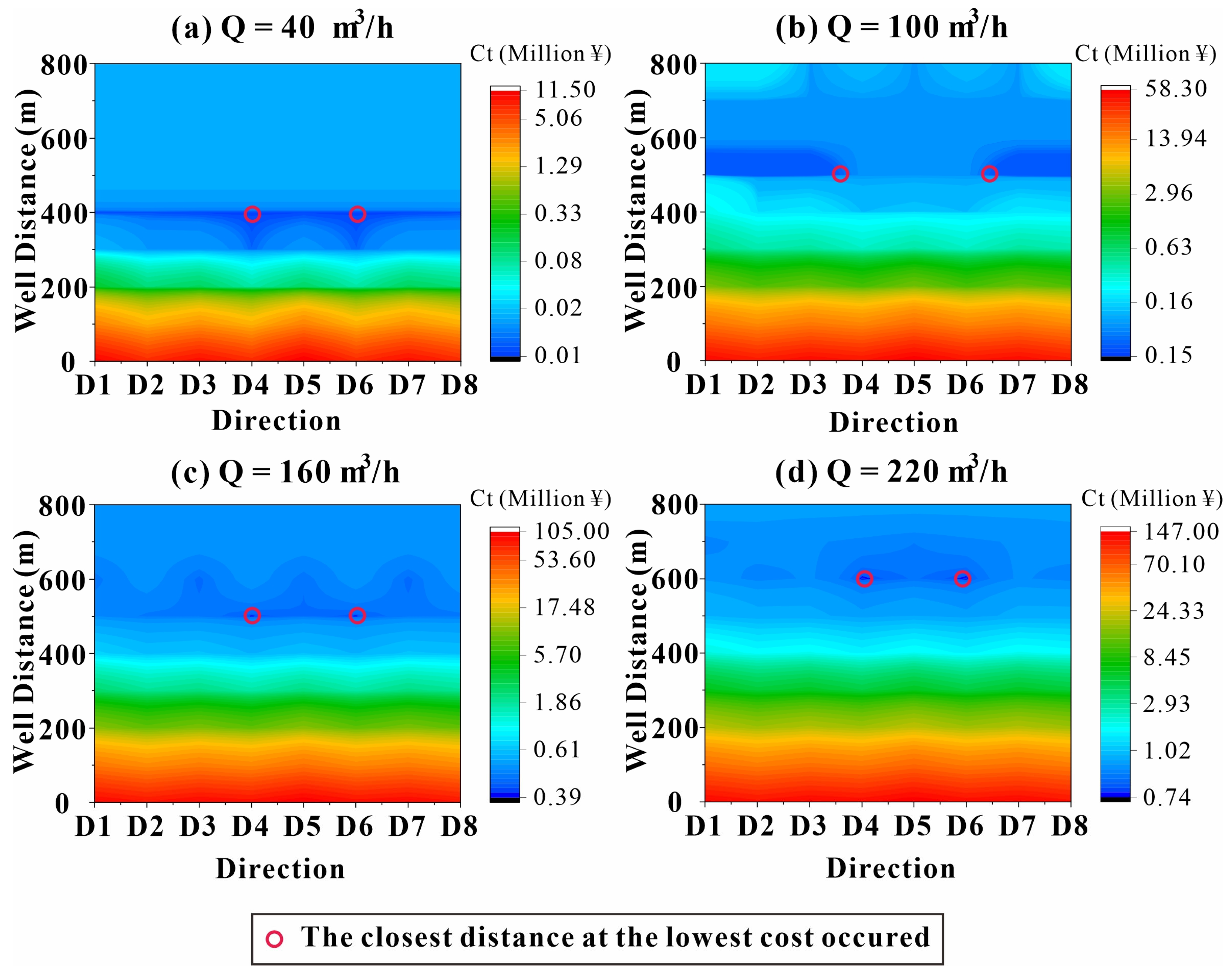
4.4. Analysis of Total Cost

The simulated temperature and pressure values of each scheme in 50 years and the current index economic standard value (

Table 2. Value of total operating cost calculation parameters [43,44,45,46].

Parameters/Unit	Values	Unit
Depreciation rate	0.08
Electricity price	0.515	¥/kwh
Heat price	70	¥/GJ
Thermal utilization ratio	0.7

) of the study area are substituted into the objective equation Ct. The total operating cost of each scheme in this period is obtained.

There are great differences in operating costs among different schemes within 50 years, especially the maximum cost of each scheme. The $Cv$ value is 2.3 and the maximum difference is 2595 times. For different well distances in the same direction, the maximum and minimum values are also tens or hundreds of times different. Therefore, it is necessary to carry out the economic analysis and reasonable optimization of each well placement scheme.

For the scheme with different well distances in the same direction, the operating cost tends to decrease at first, and then becomes stable. But, the minimum value, which is lower than the stable value, often appears before stabilization, that is, the optimal distance of the scheme. This minimum value appears between 400 m and 600 m and increases with the increase in injection flow (Figure 6). In different directions, the operating cost is still positively correlated with the injection flow. Additionally, at different distances, there is a minimum in the direction of 4 and 6 (located downstream of the production well and 45° angle to the direction of the groundwater flow field). That is to say, the stagger placement relative to the direction of the groundwater flow field is helpful to save costs.

It is worth noting that when the well distance exceeds a certain threshold, the operating cost is the same in all directions, and it is not far from the minimum cost. However, this is not the case. From the equation $Ct$ itself, this result is related to the physical properties of geology, especially the temperature and pressure at the bottom of the production well. As mentioned before, the reservoir pressure decreases significantly with the increase in well distance. This will greatly increase the cost of the pressurized injection of wastewater. Therefore, the well distance should be as small as possible. However, in order to take into account environmental protection, sustainable exploitation, and thermal breakthrough avoidance, it is necessary to increase the well distance. They contradict each other. Therefore, it is not comprehensive to consider only the economic benefits when optimizing the well placement. The evolution of reservoir temperature and pressure should be analyzed adequately.

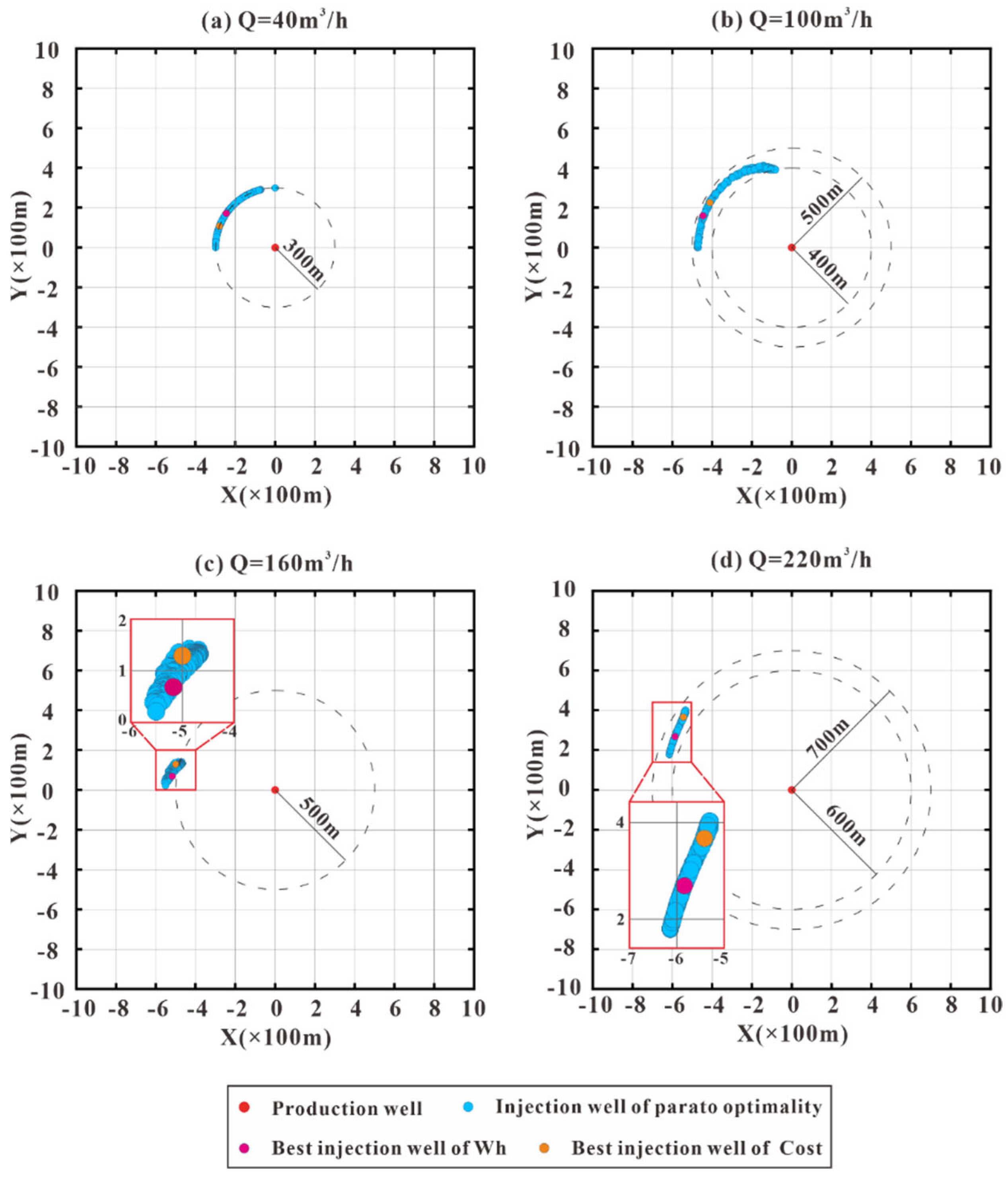
4.5. Optimal Well Placement

The production flow (injection flow) set in the scheme ranges from 40 m³/h to 220 m³/h. On the premise of considering the actual production situation, the following optimization principles are put forward:

(1)

There is no thermal breakthrough effect in the reservoir, and the temperature change threshold is 0.1 °C over 50 years;

(2)

Under the condition of satisfying (1), the pressure reduction of the reservoir is as small as possible;

(3)

Under the condition of satisfying (1) and (2), the heat extraction rate is as high as possible;

(4)

Under the condition of satisfying (1), (2), and (3), the operating cost is as low as possible.

Through the above principles, this study finally identified a pair of schemes in each representative flow rate as the optimal schemes. They are all located in the direction of D4 and D6, respectively. The optimal well distances under flow rates of 40 m³/h, 100 m³/h, 160 m³/h, and 220 m³/h are 300 m, 400 m, 500 m, and 700 m, respectively. Additionally, the evaluation indexes of the 160 m³/h flow rate group are better than others. Under the current social and economic situation in China, the injection well is located 500 m downstream of the production well. It is clamped at a certain angle with the direction of the underground flow field, and the well distance varies with the change in production (injection) flow rate.

5. Discussion

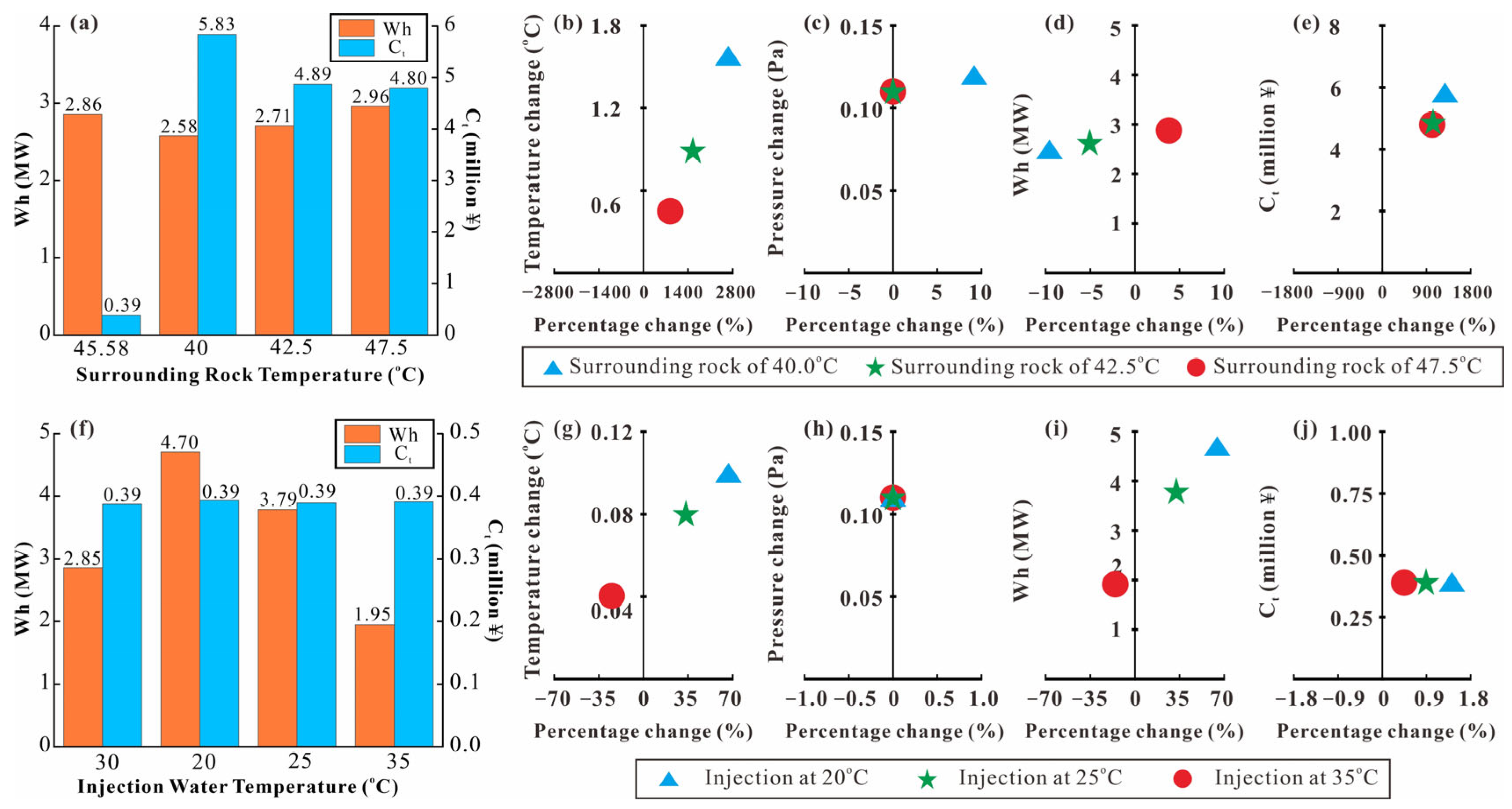
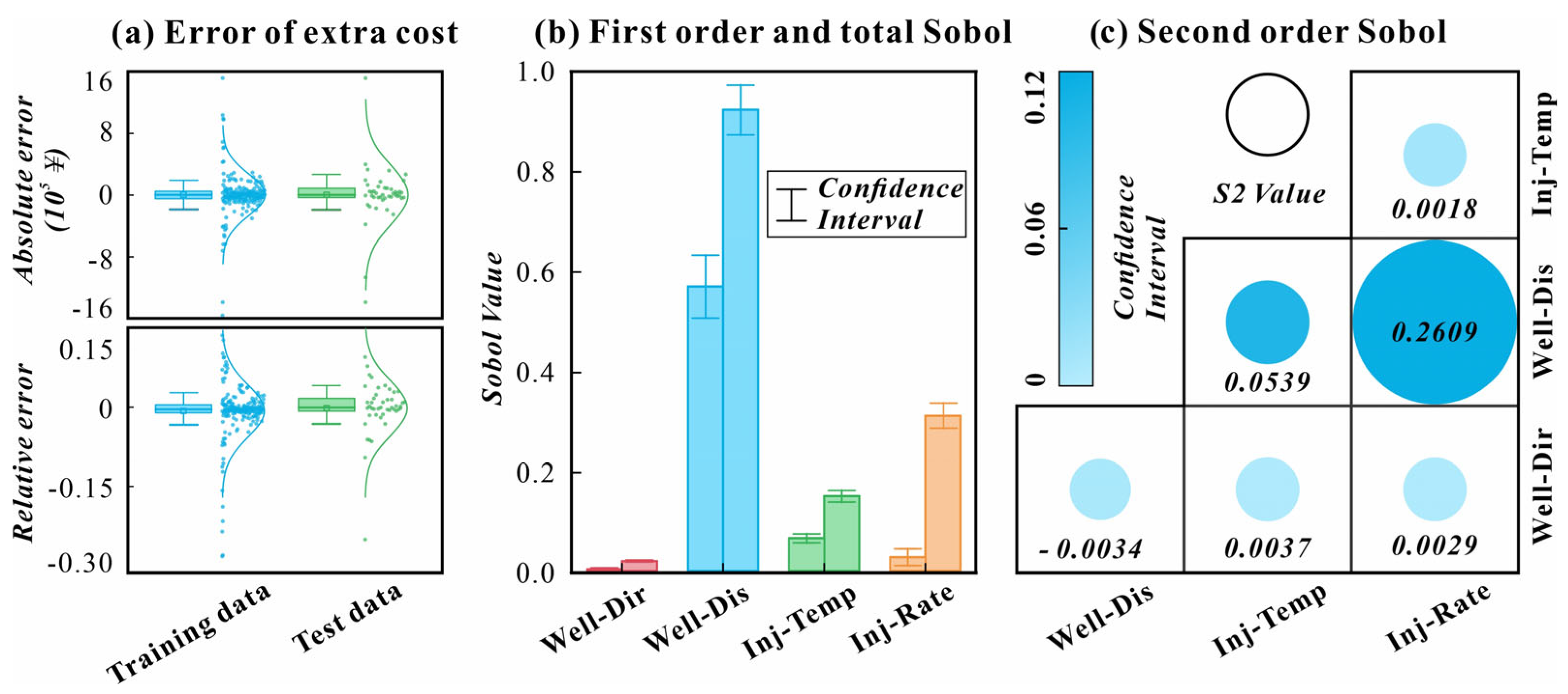
5.1. Sensitivity Analysis

It is important to understand the response degree of the hydro–thermal coupling model to hydrogeological parameters and thermophysical parameters comprehensively. In addition, it is significant to further determine the series of variables for BPNN. This study uses the optimal scheme above as the normal group. The injection flow rate is 160 m³/h, the surrounding rock temperature is 45.58 °C, and the injection temperature is 30 °C. A sensitivity analysis is performed by controlling a single variable.

(1)

Surrounding rock temperature

The change in surrounding rock temperature will directly affect the thermal field distribution and produced water temperature of the exploited reservoir through the heat conduction effect. In order to accord with the actual situation, the change gradient of the surrounding rock temperature of each scheme is small. Under the condition of no change in other parameters, three experimental groups are set up, which are 40 °C, 42.5 °C, and 47.5 °C, respectively. This study monitors the changes in temperature and pressure of a production well unit in the next 50 years, and then calculates the total operating cost in this period. Finally, the simulation results of the experimental groups and the normal group were compared.

During the 50 years of monitoring, compared with the normal group, the temperature changes of the three experimental groups were +1.54 °C, +0.85 °C, −0.53 °C, respectively, and all lead to the thermal breakthrough phenomenon. The change in reservoir pressure increased by 36.4% in the 40 °C group. The operating costs of the three experimental groups were 9.3, 7.8, and 7.7 times that of the normal group, respectively. The thermal extraction efficiency of the three experimental groups was 0.9, 0.95, and 1.04 times higher than that of the normal group (Figure 7a). The heat conduction of surrounding rock to the reservoir causes the temperature of the entire reservoir to change in different experimental groups. This significantly affects the water production temperature. The pressure field is less affected. The change of surrounding rock temperature has a great influence on the operating cost.

The change in the percentage of the main parameters is shown in Figure 7b–e. The temperature change and total cost have a great change. The larger surrounding rock temperature change tends to have larger variations. In addition, the four parameters considered respond more strongly to low-temperature surrounding rock. To sum up, a small change in the temperature of the surrounding rock will cause a significant change in the temperature and pressure of the reservoir during exploitation. This will greatly increase the operating cost. So, in production, it is significant to try to find out the temperature of the adjacent thermal reservoir and fully consider whether there are changing factors. Therefore, the influence of surrounding rock temperature should be considered when constructing BPNN.

(2)

Injection water temperature

The temperature of injection tail water is generally lower than the reservoir temperature, and a low-temperature front will be formed after entering the reservoir. Its migration and evolution will affect the temperature distribution in the reservoir and may lead to thermal breakthroughs. Under the condition of no change in other parameters, three experimental groups are set up, which are 20 °C, 25 °C, and 35 °C, respectively. This study monitors the changes in temperature and pressure of a production well unit in the next 50 years, and then calculates the total operating cost in this period. Finally, the simulation results of the experimental groups and the normal group were compared.

In the 50 years of monitoring, compared with the normal group, the temperature changes of the three experimental groups were +0.04 °C, +0.02 °C, and −0.02 °C, respectively, and there was no thermal breakthrough and almost no change in reservoir pressure (Figure 7f). The maximum variation in the operating cost was only 0.53%. The thermal extraction efficiency was 1.65, 1.33, and 0.68 times of the normal group, respectively. It can be seen that although the low-temperature tail water tends to migrate to the production well, it does not affect the temperature of the production well. The pressure field is less affected. The recharge temperature will affect the heat extraction efficiency to a greater extent, which is very disadvantageous to the efficient utilization of geothermal resources.

The change in the percentage of main parameters is shown in Figure 7g–j. The temperature change and Wh have a great change relative to the normal group. In addition, the lower injection water temperatures tend to have larger variations. To sum up, the change in injection temperature has little influence on the reservoir, but has a great influence on the thermal extraction efficiency. Therefore, the effect of recharge temperature should be fully considered in the training of BPNN.

5.2. Setup and Structure of BPNN

The simulation results were analyzed, considering engineering economy and technical feasibility. Based on this, the following input and target series variables are set for neural network learning:

(1)

Input series: angle (°), well distance (m), injection temperature (°C), and injection flow rate (m³/h);

(2)

Target series: the stable temperature at the production well (°C), stable pressure at the production well (Pa), heat extraction rate (MW), and total operating cost (million ¥).

To better solve the multi-dimensional problem of the above data series, this work chooses a two-layer feedforward structure. It uses S-shaped hidden layer neurons and linear output layer neurons. The ‘Bayesian Regularization’ back propagation algorithm is used to train the BPNN. Because of the complexity of the input series and output series in dimension and numerical scale, we set the number of hidden layer neurons to 15.

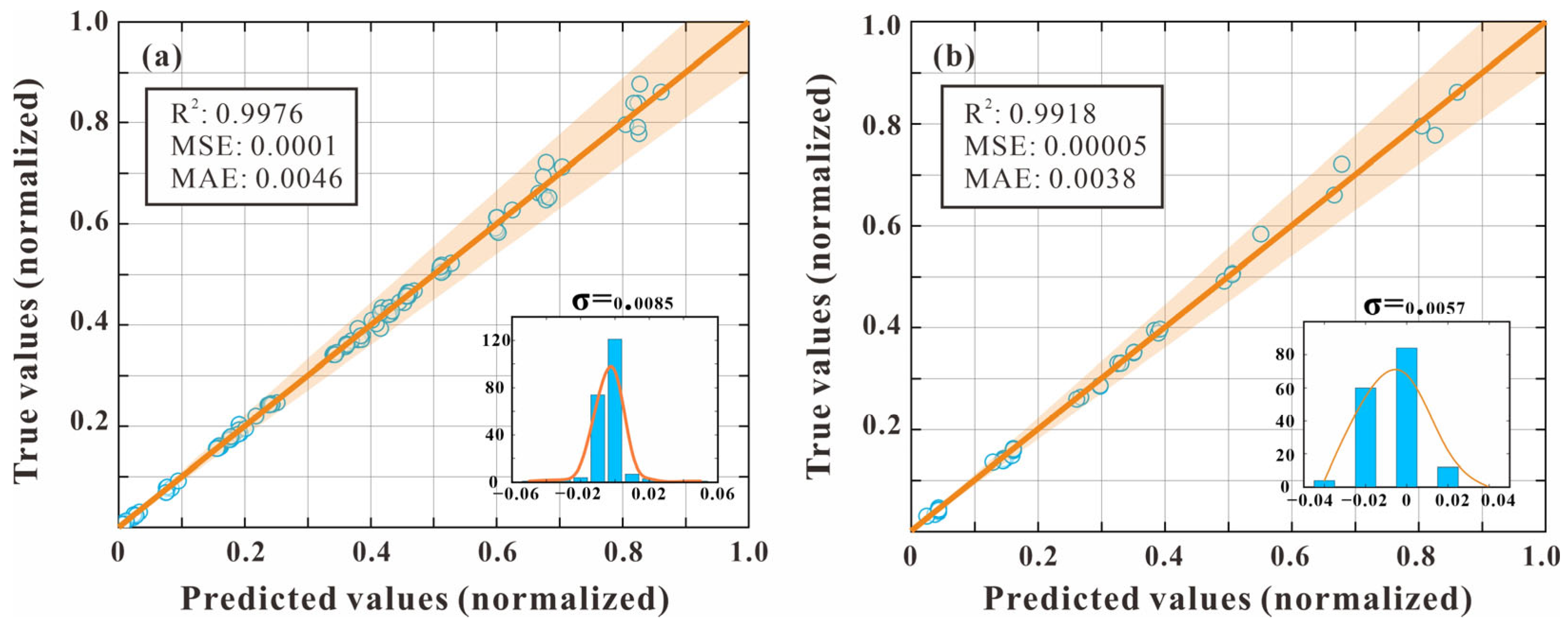
5.3. BPNN Learning Process and Results

Before training, the sample data were preprocessed. The Latin hypercube sampling method was applied in order to improve the representativeness and the balance in distribution as well as to filter out the noise of samples. Furthermore, the data sampled were normalized by min–max normalization.

The three parameters of R-Square (R²), mean squared error (MSE), and mean absolute error (MAE) were applied to evaluate the performance of the surrogate model form BPNN. The functions of them are shown in Equations (6)–(8) [47]:

$$R^2=1-{\displaystyle \frac{{\sum }_{i=1}^n{\left(y_i-\widehat{y_i}\right)}^2}{{\sum }_{i=1}^n{\left(y_i-\overline{y}\right)}^2}}$$

(6)

$$MSE={\displaystyle \frac{1}{n}}\sum _{i=1}^n{\left(y_i-\widehat{y_i}\right)}^2$$

(7)

$$MAE={\displaystyle \frac{1}{n}}\sum _{i=1}^n\left|y_i-y_i\right|$$

(8)

where $n$ is the capacity of scheme, $y_i$ is the observed value, $\widehat{y_i}$ is the predicted value, and $\overline{y}$ is the average value.

After training, the R² of the substitution model is 0.9976, and most of the samples are near zero error (Figure 8a). The mean square error reaches the minimum value of 0.0001 in the 640 iterations. The multi-dimensional fitting degree of the input series and the target series in the optimization model is very high, and the error is within the acceptable range.

In the further test, the R² (Figure 8b) of the model to the test scheme is 0.9918. The error distribution is also reasonable, and the error of most schemes is less than 0.04. This also shows that the optimization model obtained by BPNN has good performance and good prediction for different input schemes.

For the model’s prediction results, from the boxplot results of model errors, see Figure 9a. For the absolute errors, the model’s absolute errors are concentrated around zero during both the training and testing periods, with 25–75% of the errors falling within a flat box, indicating that the overall error is relatively small. During the testing period, although the overall error slightly increased, it remained within a small range, and the errors were still concentrated around zero. For the relative errors, there is an overall tendency for the errors to be lower than the predicted values, which serves as a complementary expression of the absolute error pattern. However, the relative errors generally stay within ±0.15. In conclusion, the BPNN predictions exhibit some bias, with the predicted values tending to be smaller than the actual values. Nonetheless, most errors are concentrated around zero, which is acceptable for practical applications.

Additionally, a Sobol sensitivity analysis was conducted on the model’s input features. This helps understand the trend of input data utilization and the extent to which the surrogate model substitutes for the physical process. The results are shown in Figure 9b,c. From the perspective of individual inputs, well distance made the most significant contribution to the model’s results. Injection temperature and injection flow followed, while the injection direction had a minimal impact. When considering feature interactions in the overall metrics, the influence of injection flow significantly increased. The effect of injection temperature also showed some increase, while the influence of injection direction remained small. According to the second-order Sobol interaction contribution results, the interaction between injection temperature, injection flow, and well distance amplified their contribution to the model’s output. In other words, changes in well distance enhanced the effect of injection temperature and injection flow on the results.

The fitting evaluation results of the BPNN model indicate that the surrogate model performs well in terms of prediction accuracy and error control, with an accuracy of 0.99 during the testing period. However, for the same problem, evaluating the model’s performance in isolation is one-sided. It is necessary to compare it with similar methods to assess whether there is any superiority. Among the popular machine learning algorithms, there are three main types of regression models: kernel-based models, decision tree-based models, and neural network-based models. Each of these exhibits its own advantages in different regression tasks. The BPNN used in this study belongs to the neural network architecture. Therefore, this study also introduces two models for a comparative analysis: the kernel-based Support Vector Machine (SVM) and the decision tree-based Random Forest (RF), with results shown in

Table 3. Evaluation results of surrogate models with different architectures.

Phrase	Models	$\mathit{M}\mathit{A}\mathit{E}$	$\mathit{M}\mathit{S}\mathit{E}$	$\mathit{M}\mathit{A}\mathit{P}\mathit{E}$ (×10−7)	${\mathit{R}}^2$	$\mathit{\rho }$
Training	BPNN	0.0046	0.00010	4.19	0.9976	0.9991
	RF	0.0211	0.00131	21.08	0.9702	0.9851
	SVG	0.0926	0.02249	92.63	0.4887	0.7567
Test	BPNN	0.0038	0.00005	5.76	0.9918	0.9987
	RF	0.0228	0.00189	22.82	0.8269	0.9443
	SVG	0.0681	0.00660	68.10	0.3935	0.6838

. The evaluation metrics include $MAE$, $MSE$, $R^2$, $MAPE$, and ρ, with the first three computed using Equations (6)–(8), and the latter two calculated by Equations (9) and (10) (the parameter meanings are consistent with those described earlier).

$$MAPE={\displaystyle \frac{1}{n}}\sum _{i=1}^n \left|{\displaystyle \frac{y_i-\widehat{y_i}}{y_i}}\right|\times 100\mathrm{\%}$$

(9)

$$\rho ={\displaystyle \frac{{\sum }_{i=1}^n (y_i-\overline{y})(\widehat{y_i}-\overline{\widehat{y}})}{\sqrt{{\sum }_{i=1}^n (y_i-\overline{y}{)}^2{\sum }_{i=1}^n (\widehat{y_i}-\overline{\widehat{y}}{)}^2}}}$$

(10)

In the comparison, the SVM algorithm demonstrates significant disadvantages in both error performance and prediction accuracy, with an $R^2$ value of less than 0.5 in the test set. Considering that SVMs are commonly used for linear processes, they perform poorly in non-linear processes, such as the hydrothermal process where non-linear patterns are evident. The performances of RF and BPNN are similar, with $R^2$ and ρ both exceeding 0.9 during training. However, BPNN exhibits smaller errors across all metrics and maintains stable high-level indicators during the testing period, while RF shows a significant decline in performance during the testing phase. This indicates that RF suffers from overfitting during the training process. In summary, compared to SVM and RF, BPNN demonstrates clear advantages in both error performance and prediction accuracy, with a lower degree of overfitting, making it more suitable for surrogate tasks involving complex non-linear features in hydro-thermal simulation processes.

5.4. Optimization by Genetic Algorithm

This work used a genetic algorithm to optimize the surrogate model under varied flow rates in order to further assess the accuracy and practicability of this model. Equation (11) corresponds to the optimization objective function, as follows:

$$\begin{array}{c}\mathrm{m}\mathrm{i}\mathrm{n} f\left(Q,Dis,Dir\right)=\left[-Wh,C_t\right]\\ s.t.\left\{\begin{array}{c}P\left(Q,Dis,Dir\right)-P_0⩽0.01\\ T\left(Q,Dis,Dir\right)-T_0⩽0.1\\ 0⩽Dir⩽2\pi \\ Q,Dis>0\end{array}\right.\end{array}$$

(11)

where $Q$ is the flow rate of production and injection well (m³·s⁻¹), $Dis$ is the well distance between the production well and injection well (m), $Dir$ is the counterclockwise Radian relative to east (^o), $Wh$ is the heat extract rate (MW), $C_t$ is the total economic cost (million ¥), $P$ is the pressure at the bottom of the production well (Pa), $P_0$ is the initial pressure at the bottom of the production well (Pa), $T$ is the temperature at the bottom of the production well (°C), and $T_0$ is the initial temperature at the bottom of the production well (°C).

Under the condition of four groups of representative flow rate, one set of Pareto frontier, one heat extraction rate advantage, and one economic cost advantage (Figure 10) are produced after optimization. The Pareto optimal result under different flow groups highly coincides with the findings obtained using the traditional approach. Furthermore, in engineering applications, the best well placement plan will be discovered in the Pareto front, based on site characteristics, economic conditions, and production lifespan.

5.5. Limitations of the Study

Based on BPNN and GA, this study develops a simulation-optimization approach for the placement of a well-doublet system at a particular flow rate. It has been demonstrated that the substitute model has excellent accuracy in predicting and significantly decreases the effort in the well placement optimization process. However, there are some outstanding issues in this study’s research approach:

(1)

Samples are critical for training surrogate models. Training samples of high quality and adequate capacity can facilitate the training process, increase flexibility and prediction accuracy, and minimize the problem of difficult convergence and over-fitting [48,49] of the model. In the selection of sample points, various random selection methods, such as Latin hypercube sampling [49,50], may increase the sample quality when compared to the project’s uniform division and selection. Simultaneously, the project has the potential to further minimize the change gradient and enhance sample capacity in terms of production (injection) flow rate, well distance, and injection angle setting;

(2)

In this study, a set of Pareto optimal solutions is obtained by GA optimization. Theoretically, every solution in this set is the optimal solution under the goal equation [51]. However, in engineering applications, this set of solutions must be further optimized based on individual conditions, which increases the difficulty in decision-making. There are two solutions: (a) in future work, the possible situations are written into the constraints of the GA algorithm before optimization; and (b) other more advanced and flexible multi-objective optimization algorithms, such as the wolf pack algorithm [52] and simulated annealing algorithm [53,54,55], are chosen for optimization;

(3)

In this study, the work area is chosen from the Panzhuang Uplift area in Tianjin, and the assumption of strata homogeneity is applied. Specifically, the assumption of reservoir homogeneity is not based solely on the averaging of actual site parameters, but rather an equivalent porous medium approach is used to construct the conceptual model of the experimental site. This method utilizes real pumping test results and, based on the concept of reservoir homogenization, derives the overall effect of the reservoir on the water production capacity of the production wells, which is reflected in the porosity and permeability. This approach has been widely applied in both practical engineering and research. However, as the production time increases, particularly with the injection of low-temperature tail water through injection wells, the temperature at the production well may be affected, leading to thermal breakthrough. Due to the homogenized reservoir assumption overly idealizing the diffusion process of the low-temperature tailwater plume, it neglects the impact of permeability heterogeneity on the diffusion process. As a result, there are limitations in determining the timing of thermal breakthrough. Future research will explore the effects of different pore-permeability configurations on the model, considering homogeneous, heterogeneous, and fault-affected scenarios, in order to further enhance the adaptability and accuracy of the model;

(4)

In this study, the economic calculations were based on an exit equation, which focuses on the contribution of changes in temperature and head within the reservoir to operating costs, while simplifying the impact of societal depreciation rates on the extra cost calculations. This approach is reasonable and feasible in practical engineering and economic calculations. However, since this study is primarily concerned with prediction, forecasting fluctuations in energy prices and environmental changes presents significant challenges. Due to these limitations, future research will seek to introduce alternative methods to more comprehensively consider the impacts of energy price fluctuations and environmental changes on the extra costs of well exploitation.

6. Conclusions

This study develops an approach based on a simulation-optimization model to optimize the placement of geothermal well-doublets and reduce the computational load of traditional optimization methods. The TOUGH2 program is used to construct the hydro–thermal coupling model for well-doublet production in the shallow, high-permeability thermal reservoir (Minghuazhen Formation) of the Panzhuang Uplift in Tianjin. The results of the hydro–thermal coupling model and future analyses provide sample data for training the surrogate model. Additionally, a genetic algorithm is applied to optimize the surrogate model using an objective equation that considers changes in temperature and pressure, heat extraction rate, and economic cost. The main conclusions are as follows:

(1)

An optimization strategy for the well system layout is proposed based on changes in reservoir temperature, pressure, and project operation cost. The optimal well placement for the geothermal reservoir well-doublet production system in North China is determined: the injection well should be positioned downstream of the production well, with a well distance of 500 m, and staggered relative to the natural flow field;

(2)

The simulation results from the hydro–thermal coupling model show that the production (injection) flow rate and surrounding rock temperature significantly influence the optimal well placement. When the production (injection) flow rate is high, the optimal well distance increases notably. For a production (reinjection) flow rate of 220 m³/h, the well distance can reach up to 600 m. Small changes in the surrounding rock temperature have a large impact on the geothermal fluid temperature in the production well. Therefore, it is crucial to minimize potential interference from adjacent thermal reservoir temperatures during production;

(3)

The substitution model trained by BPNN demonstrates a prediction accuracy of over 99%, with a normalized error of no more than 0.06. This model significantly reduces the calculation load and enhances portability, while providing guidance for optimizing the placement of geothermal well-doublets in geothermal reservoir production.

References

- Huenges, E.; Ledru, P. Reservoir Definition. In Geothermal Energy Systems: Exploration, Development, and Utilization; Huenges, E., Ed.; John Wiley & Sons: Hoboken, NJ, USA, 2011; Volume 1, pp. 1–2. [Google Scholar]
- Song, G.; Song, X.; Li, G.; Shi, Y.; Wang, G.; Ji, J.; Xu, F.; Song, Z. An integrated multi-objective optimization method to improve the performance of multilateral-well geothermal system. Renew. Energy 2021, 172, 1233–1249. [Google Scholar] [CrossRef]
- Limberger, J.; Boxem, T.; Pluymaekers, M.; Bruhn, D.; Manzella, A.; Calcagno, P.; Beekman, F.; Cloetingh, S.; van Wees, J.-D. Geothermal energy in deep aquifers: A global assessment of the resource base for direct heat utilization. Renew. Sustain. Energy Rev. 2018, 82, 961–975. [Google Scholar] [CrossRef]
- Bu, X.; Ran, Y.; Zhang, D. Experimental and simulation studies of geothermal single well for building heating. Renew. Energy 2019, 143, 1902–1909. [Google Scholar] [CrossRef]
- Li, F.; Guo, X.; Qi, X.; Feng, B.; Liu, J.; Xie, Y.; Gu, Y. A Surrogate Model-Based Optimization Approach for Geothermal Well-Doublet Placement Using a Regularized LSTM-CNN Model and Grey Wolf Optimizer. Sustainability 2025, 17, 266. [Google Scholar] [CrossRef]
- Lei, H.; Zhu, J. Numerical modeling of exploitation and reinjection of the Guantao geothermal reservoir in Tanggu District, Tianjin, China. Geothermics 2013, 48, 60–68. [Google Scholar] [CrossRef]
- Li, S.; Wen, D.; Feng, B.; Li, F.; Yue, D.; Zhang, Q.; Wang, J.; Feng, Z. Numerical optimization of geothermal energy extraction from deep karst reservoir in North China. Renew. Energy 2023, 202, 1071–1085. [Google Scholar] [CrossRef]
- An, Q.; Wang, Y.; Zhao, J.; Luo, C.; Wang, Y. Direct utilization status and power generation potential of low-medium temperature hydrothermal geothermal resources in Tianjin, China: A review. Geothermics 2016, 64, 426–438. [Google Scholar] [CrossRef]
- Akin, S. Geothermal re-injection performance evaluation using surveillance analysis methods. Renew. Energy 2019, 139, 635–642. [Google Scholar] [CrossRef]
- Ding, J.; Wang, S. 2D modeling of well array operating enhanced geothermal system. Energy 2018, 162, 918–932. [Google Scholar] [CrossRef]
- Cheng, W.; Wang, C.; Nian, Y.; Han, B.; Liu, J. Analysis of influencing factors of heat extraction from enhanced geothermal systems considering water losses. Energy 2016, 115, 274–288. [Google Scholar] [CrossRef]
- Murphy, H.; Brown, D.; Jung, R.; Matsunaga, I.; Parker, R. Hydraulics and well testing of engineered geothermal reservoirs. Geothermics 1999, 28, 491–506. [Google Scholar] [CrossRef]
- McDermott, C.I.; Randriamanjatosoa, A.R.L.; Tenzer, H.; Kolditz, O. Simulation of heat extraction from crystalline rocks: The influence of coupled processes on differential reservoir cooling. Geothermics 2006, 35, 321–344. [Google Scholar] [CrossRef]
- Jiang, P.; Li, X.; Xu, R.; Zhang, F. Heat extraction of novel underground well pattern systems for geothermal energy exploitation. Renew. Energy 2016, 90, 83–94. [Google Scholar] [CrossRef]
- Zeng, Y.C.; Tang, L.S.; Wu, N.Y.; Cao, Y.F. Analysis of influencing factors of production performance of enhanced geothermal system: A case study at Yangbajing geothermal field. Energy 2017, 127, 218–235. [Google Scholar] [CrossRef]
- Shaik, A.R.; Rahman, S.S.; Tran, N.H.; Tran, T. Numerical simulation of Fluid-Rock coupling heat transfer in naturally fractured geothermal system. Appl. Therm. Eng. 2011, 31, 1600–1606. [Google Scholar] [CrossRef]
- Liu, G.; Pu, H.; Zhao, Z.; Liu, Y. Coupled thermo-hydro-mechanical modeling on well pairs in heterogeneous porous geothermal reservoirs. Energy 2019, 171, 631–653. [Google Scholar] [CrossRef]
- Zhou, X.; Gao, Q.; Chen, X.; Yu, M.; Zhao, X. Numerically simulating the thermal behaviors in groundwater wells of groundwater heat pump. Energy 2013, 61, 240–247. [Google Scholar] [CrossRef]
- Asai, P.; Panja, P.; McLennan, J.; Deo, M. Effect of different flow schemes on heat recovery from Enhanced Geothermal Systems (EGS). Energy 2019, 175, 667–676. [Google Scholar] [CrossRef]
- Schulte, D.O.; Arnold, D.; Geiger, S.; Demyanov, V.; Sass, I. Multi-objective optimization under uncertainty of geothermal reservoirs using experimental design-based proxy models. Geothermics 2020, 86, 101792. [Google Scholar] [CrossRef]
- Zhang, C.; Jiang, G.; Jia, X.; Li, S.; Zhang, S.; Hu, D.; Hu, S.; Wang, Y. Parametric study of the production performance of an enhanced geothermal system: A case study at the Qiabuqia geothermal area, northeast Tibetan plateau. Renew. Energy 2019, 132, 959–978. [Google Scholar] [CrossRef]
- Blank, L.; Meneses Rioseco, E.; Caiazzo, A.; Wilbrandt, U. Modeling, simulation, and optimization of geothermal energy production from hot sedimentary aquifers. Comput. Geosci. 2020, 25, 67–104. [Google Scholar] [CrossRef]
- Zhang, S.Y.; Jiang, Z.; Zhang, S.S.; Zhang, Q.; Feng, G. Well placement optimization for large-scale geothermal energy exploitation considering nature hydro-thermal processes in the Gonghe Basin, China. J. Clean. Prod. 2021, 317, 128391. [Google Scholar] [CrossRef]
- Helgason, D. Algorithm for Optimal Well Placement in Geothermal Systems Based on TOUGH2 Models. Ph.D. Thesis, Reykjavík University, Reykjavik, Iceland, 2017. [Google Scholar]
- Rajabi, M.M.; Chen, M. Simulation-optimization with machine learning for geothermal reservoir recovery: Current status and future prospects. Adv. Geo-Energy Res. 2022, 6, 451–453. [Google Scholar] [CrossRef]
- Akın, S.; Kok, M.V.; Uraz, I. Optimization of well placement geothermal reservoirs using artificial intelligence. Comput. Geosci. 2010, 36, 776–785. [Google Scholar] [CrossRef]
- Tselepidou, K.; Katsifarakis, K.L. Optimization of the exploitation system of a low enthalpy geothermal aquifer with zones of different transmissivities and temperatures. Renew. Energy 2010, 35, 1408–1413. [Google Scholar] [CrossRef]
- Zhang, L.; Deng, Z.; Zhang, K.; Long, T.; Desbordes, J.; Sun, H.; Yang, Y. Well-Placement Optimization in an Enhanced Geothermal System Based on the Fracture Continuum Method and 0-1 Programming. Energies 2019, 12, 709. [Google Scholar] [CrossRef]
- Chen, H.; Feng, Q.; Zhang, X.; Wang, S.; Zhou, W.; Geng, Y. Well placement optimization using an analytical formula-based objective function and cat swarm optimization algorithm. J. Pet. Sci. Eng. 2017, 157, 1067–1083. [Google Scholar] [CrossRef]
- Saffari, H.; Sadeghi, S.; Khoshzat, M.; Mehregan, P. Thermodynamic analysis and optimization of a geothermal Kalina cycle system using Artificial Bee Colony algorithm. Renew. Energy 2016, 89, 154–167. [Google Scholar] [CrossRef]
- Buster, G.; Siratovich, P.; Taverna, N.; Rossol, M.; Weers, J.; Blair, A.; Huggins, J.; Siega, C.; Mannington, W.; Urgel, A.; et al. A New Modeling Framework for Geothermal Operational Optimization with Machine Learning (GOOML). Energies 2021, 14, 6852. [Google Scholar] [CrossRef]
- Gudala, M.; Govindarajan, S.K. Numerical investigations on a geothermal reservoir using fully coupled thermo-hydro-geomechanics with integrated RSM-machine learning and ARIMA models. Geothermics 2021, 96, 102174. [Google Scholar] [CrossRef]
- Yu, F.; Xu, X. A short-term load forecasting model of natural gas based on optimized genetic algorithm and improved BP neural network. Appl. Energy 2014, 134, 102–113. [Google Scholar] [CrossRef]
- Zhang, B.; Guo, S.; Jin, H. Production forecast analysis of BP neural network based on Yimin lignite supercritical water gasification experiment results. Energy 2022, 246, 123306. [Google Scholar] [CrossRef]
- Zhang, J.-R.; Zhang, J.; Lok, T.-M.; Lyu, M.R. A hybrid particle swarm optimization–back-propagation algorithm for feedforward neural network training. Appl. Math. Comput. 2007, 185, 1026–1037. [Google Scholar] [CrossRef]
- Chen, M. Study on Hydro-Thermo-Mechanical Coupling Numerical Simulation of Sand-Stone Thermal Reservoir in Panzhuang Uplift Area, Tianjin City. Ph.D. Thesis, Jilin University, Changchun, China, 2020. [Google Scholar]
- Pruess, K.; Oldenburg, C.; Moridis, G. TOUGH2 User’s Guide Version 2; Lawrence Berkeley National Laboratory: Berkeley, CA, USA, 1999. [Google Scholar]
- Li, F.; Xu, T.; Feng, G.; Yuan, Y.; Zhu, H.; Feng, B. Simulation for water-heat coupling process of single well ground source heat pump systems implemented by T2well. Acta Energiae Solaris Sin. 2020, 41, 9. [Google Scholar]
- Kong, Y.; Pang, Z.; Shao, H.; Kolditz, O. Optimization of well-doublet placement in geothermal reservoirs using numerical simulation and economic analysis. Environ. Earth Sci. 2017, 76, 118. [Google Scholar] [CrossRef]
- Liu, C.; Ling, J.; Kou, L. Performance Comparison between GA-BP Neural Network and BP Neural Network. Chin. J. Health Stat. 2013, 30, 173. [Google Scholar]
- Fu, Q. Water Resources System Analysis; China Water & Power Press: Beijing, China, 2012. [Google Scholar]
- Liang, X.; Xu, T.F.; Feng, B.; Jiang, Z.J. Optimization of heat extraction strategies in fault-controlled hydro-geothermal reservoirs. Energy 2018, 164, 853–870. [Google Scholar] [CrossRef]
- National Development and Reform Commission & Ministry of Construction. Methods and Parameters for Economic Evaluation of Construction Projects, 3rd ed.; China Planning Press: Beijing, China, 2008.
- Tianjin Development and Reform Commission. Tianjin Residential and Agricultural Electricity Sales Price Meter. Available online: https://fzgg.tj.gov.cn/zmhd/gzcx/syjgcx/gd/202202/t20220217_5806380.html (accessed on 11 March 2025).
- Tianjin Development and Reform Commission. Heating Price. Available online: https://fzgg.tj.gov.cn/zmhd/gzcx/syjgcx/gr/202009/t20200923_3807284.html (accessed on 11 March 2025).
- Lund, J.W.; Freeston, D.H. World-wide direct uses of geothermal energy 2000. Geothermics 2001, 30, 29–68. [Google Scholar] [CrossRef]
- Wang, J.; Zhao, Z.; Liu, G.; Xu, H. A robust optimization approach of well placement for doublet in heterogeneous geothermal reservoirs using random forest technique and genetic algorithm. Energy 2022, 254, 124427. [Google Scholar] [CrossRef]
- Shorten, C.; Khoshgoftaar, T.M. A survey on Image Data Augmentation for Deep Learning. J. Big Data 2019, 6, 48. [Google Scholar] [CrossRef]
- Helton, J.C.; Johnson, J.D.; Sallaberry, C.J.; Storlie, C.B. Survey of sampling-based methods for uncertainty and sensitivity analysis. Reliab. Eng. Syst. Saf. 2006, 91, 1175–1209. [Google Scholar]
- Helton, J.C.; Davis, F.J. Latin hypercube sampling and the propagation of uncertainty in analyses of complex systems. Reliab. Eng. Syst. Saf. 2003, 81, 23–69. [Google Scholar]
- Zhou, A.M.; Qu, B.Y.; Li, H.; Zhao, S.Z.; Suganthan, P.N.; Zhang, Q.F. Multiobjective evolutionary algorithms: A survey of the state of the art. Swarm Evol. Comput. 2011, 1, 32–49. [Google Scholar] [CrossRef]
- Dhargupta, S.; Ghosh, M.; Mirjalili, S.; Sarkar, R. Selective Opposition based Grey Wolf Optimization. Expert Syst. Appl. 2020, 151, 13. [Google Scholar]
- He, C.L.; Yan, J.W.; Wang, S.Q.; Zhang, S.; Chen, G.; Ren, C.Z. A theoretical and deep learning hybrid model for predicting surface roughness of diamond-turned polycrystalline materials. Int. J. Extrem. Manuf. 2023, 5, 25. [Google Scholar]
- Long, F.; Liu, H. An integration of machine learning models and life cycle assessment for lignocellulosic bioethanol platforms. Energy Convers. Manag. 2023, 292, 11. [Google Scholar]
- Vijay, D.; Jayashree, R. Sliding Mode Controller Based on Genetic Algorithm and Simulated Annealing for Assured Crew Reentry Vehicle. J. Aerosp. Eng. 2023, 36, 23. [Google Scholar]