A Comparative Analysis of In-Situ Wave Measurements and Reanalysis Models for Predicting Coastline Evolution: A Case Study of IJmuiden, The Netherlands

Abstract

This study investigates the influence of wave-climate datasets derived from in situ measurements and reanalysis models on predictive modelling accuracy for coastline evolution, focusing on the IJmuiden coastal stretch in The Netherlands. By analyzing wave parameters, sediment dynamics, and nourishment interventions, the research evaluates the performance of a numerical model in simulating shoreline changes over a 40-year period. Using the LTC (Long-Term Configuration) model, scenarios incorporating artificial sand nourishment volumes of 200,000 m³/year and 250,000 m³/year were tested against conditions without nourishment. The results highlighted the critical role of significant wave height, direction, and dataset variability in sediment accretion and erosion patterns. Datasets from in situ measurements (Measured-YM6) and reanalysis sources (ERA5, AENWS-WPR, and AENWS-WPR North) demonstrate variable performance, with ERA5 proving to be the most reliable under both nourished and non-nourished scenarios. The findings emphasize the importance of integrating high-resolution wave datasets into numerical models to improve predictions, optimize nourishment strategies, and enhance coastal resilience against erosion. The study underscores the necessity of nourishment interventions to mitigate sediment loss, stabilize shorelines, and support sustainable coastal-management practices in the face of climate change.

1. Introduction

The dynamic relationship between wave climate, sediment characteristics, and availability are crucial in shaping littoral morphology. When the amount of sediment leaving a coastal stretch is balanced by the amount of sediment entering, the system is in dynamic equilibrium, resulting in neither erosion nor accretion. However, if this sediment balance is disrupted, erosion or accretion will occur, leading to the retreat or advance of the shoreline, respectively [1,2]. Beach morphology can change seasonally due to variations in wave energy and direction, and potential sediment transport. In some regions, sediment accumulation and erosion patterns are driven more by changes in sediment transport direction than wave energy [3].

Artificial sediment nourishment is an intervention strategy that has been adopted by several countries all over the world [4,5] to minimize coastal erosion problems, prevent flooding, and enable the maintenance of wide beaches that serve to recreational purposes [6,7,8,9]. Compared with other methods to protect the coastline (e.g., breakwaters, groins, seawalls), artificial sand nourishment is not only more flexible but also offers potential benefits, including safeguarding the environment and improving recreational services [10,11]. Although artificial nourishments are widely applied in different sites as a soft coastal intervention, questions related to the fill material fate, lifetime, and long-term impacts (to downdrift areas) still need to be answered with more confidence [9].

The main objective of this study was to explore the impact of in situ and reanalysis wave-climate datasets on predicting sediment distribution and shoreline evolution, following artificial nourishment interventions over 40 years, using a shoreline evolution model. Shoreline evolution models can predict sediment dispersion patterns, which are crucial for understanding sediment accumulation and erosion along coastlines. Accurately predicting shoreline evolution involves a complex interplay between in situ wave-climate data and reanalysis models. Several authors investigated the integration and impact of these data sources on the precision of predictive modelling [12,13,14,15], which is crucial for coastal management in the face of climate change and increasing frequency of extreme weather events.

Various approaches have been employed to model and predict coastline behaviour. Significant contributions to numerical modelling improvements, calibration techniques, and simplified modelling approaches for shoreline evolution prediction have been made by several authors, including [16,17,18,19,20]. These studies emphasize the necessity of accurate field data for model calibration and highlight the vulnerability of beaches to climate change-induced erosion, as noted by [21,22].

Other approaches focus on the importance of probabilistic modelling and joint estimation techniques for extreme storm events, which are crucial for disaster risk analysis and structural protection, as discussed by [23]. Various methods to predict dune erosion have been explored, such as the XBeach model, which identifies a linear relationship between sea level rise and erosion [24], and the development of a neural network-based meta-model showing promise for early warning systems [25]. Satellite-derived shoreline observations have demonstrated capabilities for fine-scale coastal change monitoring [26], and clustering techniques and typological coastal profiles have been introduced for efficient national-scale dune-erosion estimation [27].

In terms of wave climate, Ref. [28] validated the CoSMoS wave- and surge-prediction system for the Dutch coast, proving its accuracy in predicting wave parameters and surge elevation while suggesting improvements in modelling wave-swell components. Additionally, regional downscaling in statistical wave-climate projections by [12] and the use of reanalysis to improve the reconstruction of past weather and ocean states by [29] have enhanced coastline evolution modelling, aiding detailed coastal impact assessments.

A case study in IJmuiden, The Netherlands, was considered to compare the observed scenario with multiple simulated scenarios that incorporate artificial sand nourishment volumes of 200,000 m³/year and 250,000 m³/year. These scenarios were tested against conditions without nourishment, using four wave-climate datasets and applying the Long-Term Configuration (LTC) model. The performance of the nourishment depends on various factors related to sediment dynamics and the artificial sand nourishment process itself. Consequently, the study evaluated the impact of different nourishment scenarios, defined in the numerical model by varying boundary conditions and wave climates. Additionally, the patterns of the longshore transport of the nourished sediments were analyzed to anticipate their retention at the deposition site and determine the frequency required for subsequent nourishment interventions.

A detailed overview of the case-study area (IJmuiden) is provided in Section 2, followed by a description of the materials and methods, including the available datasets, the wave scenarios, a description of the LTC model, and the model setup in Section 3. The results are then presented, highlighting the key findings in Section 4. This is followed by a discussion on the importance of wave-climate data in numerical modelling simulation outcomes in Section 5. Finally, the main conclusions are outlined in Section 6.

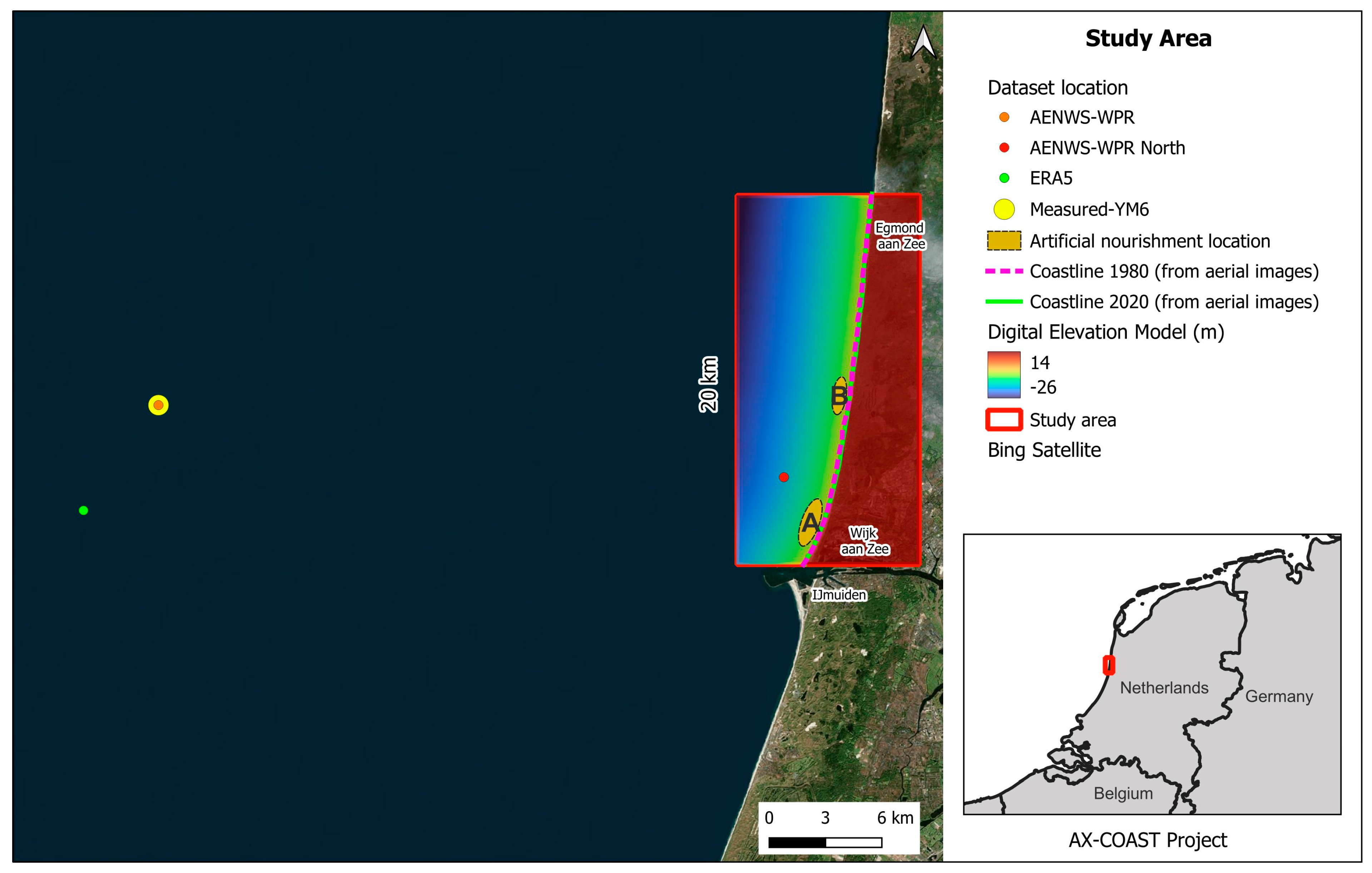
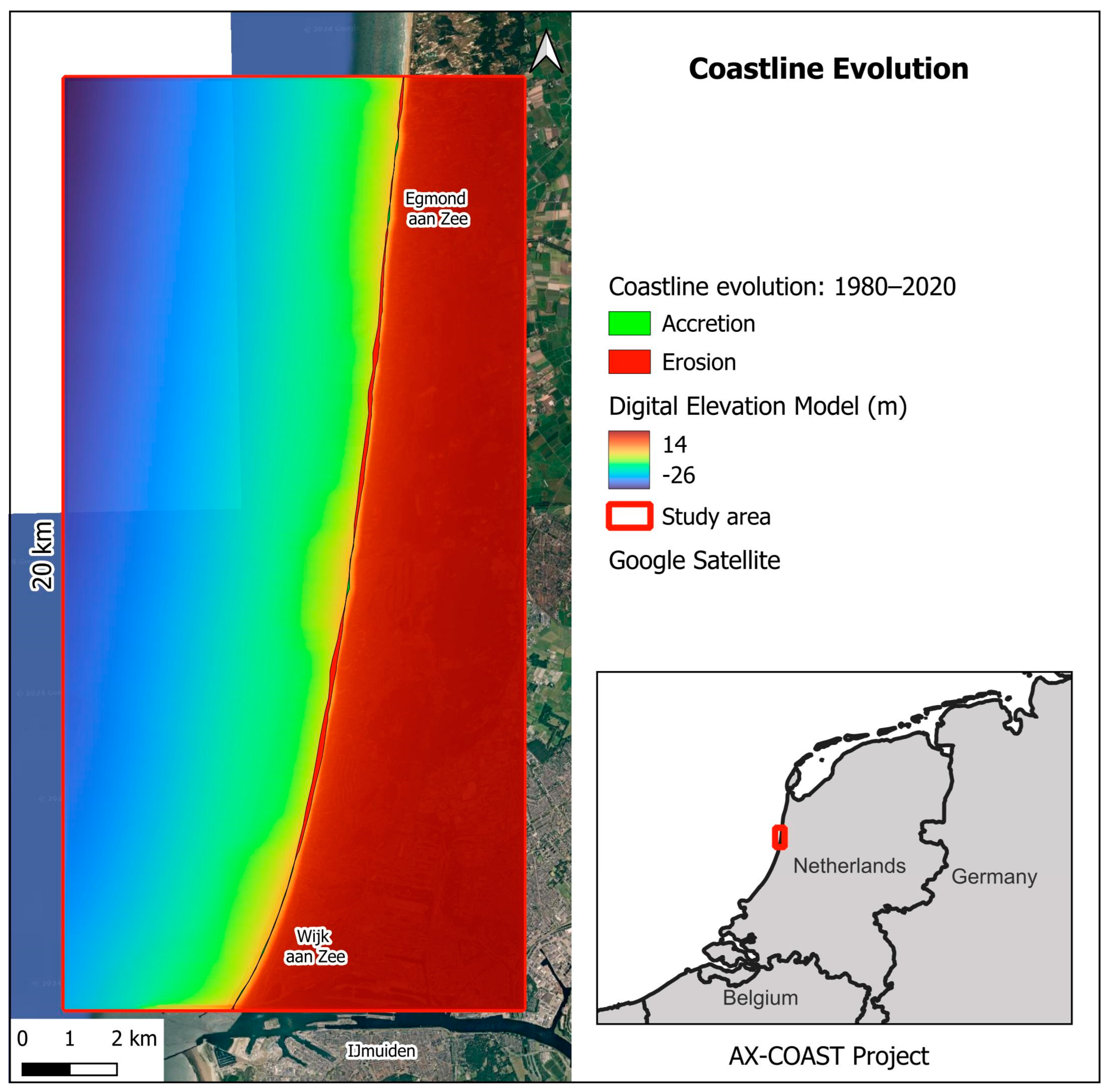
2. IJmuiden (The Netherlands) Study Area

The Netherlands has a coastline stretching of 432 km, predominantly consisting of approximately 75% sandy beaches and dunes, 15% hard structures, and 10% tidal flats [30]. This coastline is typically divided into three distinct regions: the southwest delta, characterized by multiple open and semi-enclosed estuaries; the central coast, which is relatively straight and shifts in orientation from northeast–southwest in the south to north–south in the north (known as the Holland coast); and the northern barrier-island coast, which features several barrier islands and tidal inlets [31]. The study area selected is IJmuiden (Figure 1), located in the central part of the Holland coast (The Netherlands).

In the IJmuiden coastal zone, a harbour was constructed between 1867 and 1876 to connect Amsterdam’s inner port to the North Sea via the man-made North Sea Canal. Prior to 1865, the local coastline was closed, consisting of a single row of natural sand dunes. In 1876, the harbour breakwaters extended about 1200 m seaward from the original coastline, with the seabed at the mouth of the harbour lying approximately 7 m below mean sea level (MSL).

Between 1962 and 1967, the harbour breakwaters were further extended by about 1500 m to accommodate larger vessels, positioning the tip of the southern harbour dam approximately 2800 m seaward of the 1865 coastline. The seabed at the mouth of the extended harbour breakwaters now lies about 20 m below mean sea level. The harbour construction conducts an erosion process in the north of the harbour and, the south of the harbour breakwaters has experienced significant sand accretion along an approximate 4 km stretch of the shore and up to 2 km cross-shore.

Typical wave heights in this area range between 0.1 and 1.5 m, with approximately 55.5% of waves measured during the period from January 1979 to December 2021. The predominant wave direction is from the southwest, averaging 225 degrees from the north, clockwise. The tidal wave propagates from south to north along the Dutch coast. The tidal range at IJmuiden varies from approximately 1 m during neap tide to 2 m during spring tide [32].

The peak tidal-flood current in deeper water (20 m) is about 0.65 m/s to north near IJmuiden and the peak tidal-ebb current is about 0.55 m/s to south based on calibrated model computations for mean tidal conditions (DELFT3D-model). The flow is mainly parallel to the coast, except around the harbour breakwaters of IJmuiden. During storm conditions from southwest, the peak tidal-current velocity near IJmuiden increases to 0.75 m/s during flood to north, but the peak ebb tidal-current velocity decreases to about 0.45 m/s. The breakwaters at IJmuiden harbour generate complex tidal flow patterns. Large eddies are formed by tidal currents at the harbour entrance, as well as south of the harbour during ebb tide and at north during flood tide. The strong flow contraction in front of the entrance, combined with locally intensified turbulence, has created a scour hole at the entrance. These eddies may enhance water exchange between the harbour basin and the sea, potentially increasing sediment import; see Figure 2 [33]

Alongshore sediment transport in the study area predominantly occurs from south to north. At IJmuiden, the southern beach near the southern groin experiences significant sand accretion, with an estimated rate of 115,000 to 395,000 m³ per year. In contrast, the northern beach near the northern groin is subject to erosion at a rate of approximately 40,000 m³ per year [34], although this erosion is mitigated by regular artificial sand nourishments. The annual average volume of sand nourishment along the Holland coast has increased significantly over the years, from 0.4 million m³ per year between 1952 and 1990, to 2.5 million m³ per year between 1991 and 2000, and further to about 5 million m³ per year from 2001 to the present [35]. Current annual mitigation costs are around 25 million euros, with added sand volumes ranging from 200 to 600 m³ per metre in eroding coastal stretches [35].

The IJmuiden northern coast benefits from periodic artificial nourishments around the Bergen–Egmond coastal laboratory, leading to observed accretion trends in the profile. These nourishments have been carried out since 1990, initially every two years, with deposited volumes between 60,000 and 472,640 m³. Between 1997 and 2000, annual nourishments were conducted with volumes ranging from 132,690 to 994,000 m³. During the period from 2010 to 2015, nourishments were spaced over five years, with sand volumes increasing from 300,436 m³ to 2,500,000 m³ [36]. The south groin at IJmuiden acts as a barrier to the predominant south-to-north longshore sediment transport, promoting sand accretion in the southern area. Conversely, the shadow zone of the northern groin at the IJmuiden harbour entrance anticipates an erosion trend [32].

The median sediment grain size (d50) at IJmuiden ranges between 0.20 and 0.25 mm, with alongshore sediment transport in this area estimated at approximately 180,000 m³ per year, from south to north [34].

3. Materials and Methods

Waves are a primary source of energy in the littoral zone and, along with currents, play a crucial role in coastal erosion and sediment transport. They are a fundamental force driving the modification of coastlines and the formation of both erosional and depositional landforms. Accurate wave measurements are essential for modelling and studying erosion and sediment transport, as well as for the design of seawalls, harbours, and other coastal infrastructures [37]. Wave buoy datasets have certain limitations, particularly regarding deployment durations, sampling frequency, and occasional instrument failures, especially during storms. To generate nearshore and extreme wave heights—critical for assessing potential coastal impacts—wave models are essential. They are invaluable for filling gaps in observed datasets, enhancing the understanding of extreme events, and providing wave-condition forecasts. However, a significant challenge in many regions is the lack of local data, which hinders the calibration and verification of modelled results.

The state of the art includes several studies focused on understanding and projecting wave climate to assess future coastal risks [12,13,14,15]; shoreline evolution modelling, particularly in relation to sediment dynamics and beach profile changes [17,19,20]; the importance of monitoring and modelling morphological changes in coastlines for sustainable management [16,18]; and the critical role of understanding beach response to storm events in evaluating coastal vulnerability [21,22].

This study evaluates the performance of the LTC—Long-Term Configuration [2] numerical model in reproducing historical coastline evolution over the period 1980–2020. To achieve this, four wave-climate datasets—including in situ measurements, as well as offshore and nearshore reanalysis data, as described in Section 3.1—are used to force the model. The model outputs are then compared with observed coastline changes to assess its accuracy in simulating past shoreline retreat and position. By integrating multiple wave-data sources, this approach seeks to verify the reliability and robustness of the numerical modelling results in relation to real-world observations.

The methodology developed in this work is based on three main phases (Figure 3): (i) Baseline definition, which includes a wave dataset analysis, a shoreline reference scenario definition and evaluation; (ii) shoreline modelling and evolution projection in a medium-term horizon applying LTC (Long-Term Configuration) numerical model [2]; and (iii) the model results—a coastline evaluation analysis for each scenario (12 scenarios) and morphological results vs. wave dataset analysis. The methodology is described in the following sections.

3.1. Materials

3.1.1. Wave-Climate Data—In Situ and Reanalysis Dataset Characterization

Wave-climate datasets derived from global and regional wave models were collected for the IJmuiden area to assess the impact of different data sources on the model results. The datasets used include in situ data Measured-YM6, reanalysis data from the global ERA5 model [38] and hindcast simulations from the regional AENWS-WPR model [39]. Measured-YM6 wave-climate data were collected from an offshore station located 26 km from the IJmuiden coast, at a depth of 21 m (52.55° N, 4.06° E, water depth ≈ 25 m to MSL) [23]. The ERA5 dataset corresponds to an area of 0.25° × 0.25°, represented by its central point, located near to the initial measurement site, Measured-YM6 (ERA5: 52.50° N, 4.00° E), while the AENWS-WPR model provided wave-climate data for Measured-YM6 (52.55° N, 4.06° E) and one additional nearshore location north (AENWS-WPR North) of IJmuiden (52.51° N, 4.55° E) [32]. The positions of these datasets are illustrated in Figure 1, and significant wave height, peak wave period, and the direction for each dataset are presented in Figure 4.

Observing Figure 4, the significant wave-height distribution reveals that the majority of waves fall within the 0–2 m range. The AENWS-WPR North dataset (orange) reports a particularly high frequency of waves in the 0–1 m interval, whereas the Measured-YM6 (blue) and ERA5 (green) datasets exhibit a more balanced distribution across the 0–2 m range.

The distribution of peak wave periods reveals that most waves fall within the 4–8 s range, with the 4–6 s interval being the most prevalent across all datasets. The Measured-YM6 dataset (blue) exhibits the highest frequency in this range, followed closely by ERA5 (green). As the peak wave period extends beyond 8 s, the frequency of occurrence drops significantly, indicating that longer peak wave periods are generally less common in the recorded data. However, it is notable that the reanalysis datasets, show a higher frequency of peak wave periods, exceeding 8 s when compared to the Measured-YM6 (blue).

The wave direction distribution highlights a clear dominance of waves coming from the southwestern sectors (SW, WSW, W) and northwestern sectors (WNW, NW, NNW, N). These directions show the highest frequencies, particularly in the SW and NNW sectors. AENWS-WPR North (orange) and Measured-YM6 (blue) are particularly prominent from the SW, WSW, and NNW directions, while ERA5 (green) and AENWS-WPR (red) show a consistent presence across multiple sectors. Across all wave datasets, a consistent pattern in wave direction is observed, with waves predominantly propagating from south to north between September and January, when significant wave heights are at their peak, and from north to south between April and August, when waves are smaller (Figure 4 and Figure 5). Additionally, the AENWS-WPR North dataset (orange) displays a relatively narrower range of wave directions, with waves tending to be more perpendicular to the coastline. The eastern to southern sectors (ENE, E, ESE, SE, SSE, S), which correspond to directions from land, exhibit negligible frequencies, as expected. This indicates that these directions contribute less to the overall wave climate in the recorded data. The consistent dominance of the southwestern–western and northwestern directions suggests a prevailing wind and wave pattern from these directions.

The slight variability observed between the datasets likely reflects differences in data collection/reanalysis methods and locations, yet overall, the trends remain largely consistent.

A statistical analysis of the wave climate is summarized in

Table 1. A statistical analysis of the wave-climate datasets.

Parameters	Dataset	Min	Mean	Max/Main D (°)	Std	Percentile *
						25th	50th	75th	90th	99th
Hs (m)	Measured-YM6	0.09	1.27	7.17	0.83	0.66	1.07	1.66	2.40	4.06
	ERA5	0.04	1.20	7.47	0.79	0.63	1.00	1.56	2.29	3.84
	AENWS-WPR	0.03	1.24	6.72	0.76	0.68	1.08	1.65	2.32	3.55
	AENWS-WPR North	0.02	0.94	4.56	0.64	0.44	0.78	1.28	1.84	2.89
Tp (s)	Measured-YM6	1.79	5.68	22.97	1.35	4.81	5.67	6.54	7.35	9.05
	ERA5	1.83	5.97	19.35	1.85	4.73	5.79	6.90	8.18	12.00
	AENWS-WPR	1.65	6.33	18.85	1.97	5.05	6.18	7.42	8.75	12.42
	AENWS-WPR North	1.65	6.42	19.52	2.13	5.04	6.22	7.56	9.06	13.35
D (°)	Measured-YM6	-	235.67	WSW-SW	104.57	-
	ERA5	-	222.97	SW	110.14
	AENWS-WPR	-	230.65	SW	112.83
	AENWS-WPR North	-	275.97	W	77.96

Notes: * Percentile: A percentile is a statistical measure that divides an ordered dataset into 100 equal parts, with each percentile representing a percentage of the distribution. For example, the 50th percentile (median) indicates that 50% of the data fall below this value, while the 25th, 75th, 90th, and 99th percentiles show where 25%, 75%, 90%, and 99% of the data lie, respectively.

, highlighting the main differences between the datasets. The maximum significant wave height ranges from 4.56 m at the AENWS-WPR North shoreline dataset to 7.47 m at the ERA5 offshore dataset, reflecting the higher energy conditions captured offshore by ERA5. The mean peak wave period is generally higher in reanalysis datasets, with Measured-YM6 presenting the highest maximum peak wave period, indicating more frequent longer waves in this dataset. Mean wave direction varies slightly across the datasets but consistently points to SW or WSW, aligning with the observed dominance of these directions in the wave climate.

Analyzing in detail the significant wave-height distributions using various percentiles of occurrence, summarized in Table 1, reveals that the nearshore dataset (AENWS-WPR North) consistently exhibits lower significant wave heights compared to the offshore datasets (Measured-YM6, ERA5, and AENWS-WPR). This reduction in significant wave height nearshore is expected, as waves lose energy due to interactions with the seabed and coastal features as they approach to the shoreline. Additionally, it is also observed that the mean wave direction in the nearshore dataset (AENWS-WPR North) is from the west (W), which is nearly perpendicular to the coastline.

When comparing the offshore datasets, the analysis reveals that the differences in significant wave height become more pronounced at higher percentiles (90th and 99th). This suggests that the offshore datasets capture extreme wave events with varying degrees of accuracy. However, when directly comparing the measured significant wave heights at Measured-YM6 with the modelled heights from ERA5 and AENWS-WPR, no consistent trend emerges. The models do not systematically overestimate or underestimate significant wave heights (e.g., 25th and 50th) relative to the measured values, indicating that both ERA5 and AENWS-WPR provide reasonably accurate representations of wave conditions in this region.

Nevertheless, a general pattern can be observed: the models tend to underestimate significant wave heights (Hs)—as the measured mean and percentile values are consistently higher than those predicted by the models—and overestimate peak wave periods—since the measured mean and percentile values of Tp are consistently lower than the modelled results.

A detailed monthly analysis of the wave dataset (Figure 5) reveals distinct seasonal patterns in wave direction. During the autumn and winter months (October–March), waves predominantly originate from the southwest/west quadrant, while in the spring and summer months (April–September), the dominant wave direction shifts to the north–northwest quadrant. This seasonal variation in wave direction is closely mirrored by changes in significant wave height, which also exhibits higher values during the autumn–winter period and lower values in the spring–summer period.

Additionally, the peak wave period analysis indicates that higher values are consistently associated with waves from the north–northwest quadrant across all datasets. However, the reanalysis datasets, particularly the AENWS-WPR North dataset, generally report higher mean peak wave periods compared to the other datasets. This suggests that the reanalysis models may capture longer-period waves more frequently, possibly due to their ability to represent broader, more distant wave-generated storms.

3.1.2. Forcing Agents Scenarios

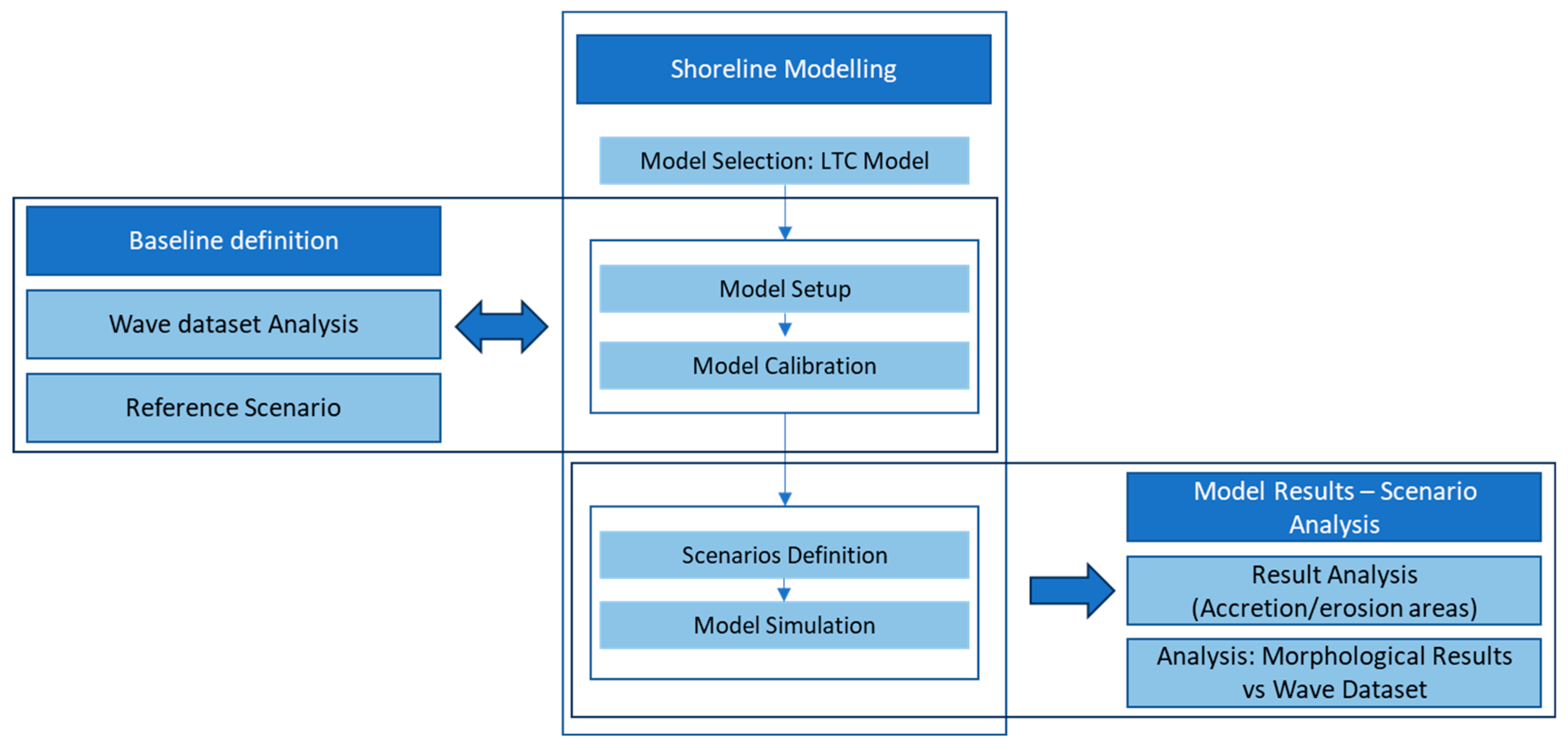
The wave-climate data used were from the Measured-YM6 dataset, covering the period from 1980 to 2020 (with the full time series available from 1971 to 2022), as well as three reanalysis datasets: one from global ERA5 model [38] and two hindcast simulations, from the regional AENWS-WPR model [39] (one point near Measured-YM6 and the other close to the coast); see Figure 6.

The four wave datasets are 3 h intervals, over 40 years. The wave-climate data include the significant wave height (Hs) in metres, the peak wave period (Tp) in seconds, the wave direction (Dir) in degrees (measured clockwise from north), and the tide levels (tide) in metres. Regarding direction, considering the orientation of the coastal zone under study, the datasets Measured-YM6, ERA5 and AENWS-WPR on average present an oblique wave-incidence direction, 235.67°, 222.97° and 230.65°, respectively, whereas the dataset AENWS-WPR North presents, on average, a wave incidence perpendicular to the shoreline (275.97°). The tide-range data considered were the mean value, 1 m, based on the records from this area.

3.2. Methods

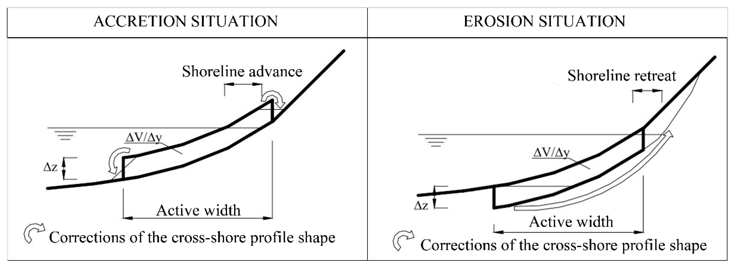
3.2.1. LTC Numerical Model Description

Numerical modelling is an important tool in the coastal management process, allowing for the comparison of solutions and the prioritization of intervention measures. There are several coastal-zone evolution models, but due to the complexity of the processes involved, each model focuses on specific processes. The model-selection results from the balance between the time scale of the analysis and the most relevant coastal processes observed at that scale.

This study applies the LTC, Long-Term Configuration model [2], which is a shoreline model for sandy beaches and integrates a basic classical one-line model with a rule-based model for the distribution of erosion and accretion volumes along the beach profile [9,40,41]. This model allows the user to simulate different coastal erosion protection and adaptation interventions, such as artificial sand nourishment, groins, revetments, alluvial point sources and detached breakwaters [42,43].

The LTC numerical model assumes that each wave acts individually over a specific time period, corresponding to the computational time step. For each wave, the model’s computational structure performs three main steps: (1) wave propagation; (2) calculation of the longshore sediment transport volume; and (3) updating beach morphology based on longshore sediment transport gradients.

The model accounts for refraction and shoaling phenomena during wave propagation, as well as diffraction near coastal structures. Wave breaking occurs when the water depth reaches approximately Hb ≈ 0.78 hb, where Hb is the significant wave height and hb is the local depth at the breaking point.

Based on one-line theory, the LTC model simulates medium- to long-term coastal configuration evolution by applying the sediment continuity equation (Equation (1)). In this equation, $V$ represents the volume of sediments in a section of infinitesimal width ($\partial y$), $Q$ is the longshore sediment transport rate, $q_x$ denotes any external sediment supplies (such as artificial nourishments) per unit of beach width, and $t$ represents the time [2].

$${\displaystyle \frac{\partial V}{\partial t}}=\left({\displaystyle \frac{\partial Q}{\partial y}}+q_x\right)$$

(1)

According to Coelho [2], discretizing Equation (1) into time intervals ($∆t$) and applying it along the shoreline for stretch of length ($∆y$) allows for relating the volume variation in each stretch to the temporal variation in longshore sediment transport:

$$∆V=\left(Q_i-Q_{i-1}+Q_{ext}\right)∆t=\left(∆Q+Q_{ext}\right)∆t$$

(2)

The variation in longshore sediment transport over the length ($∆y$) results from the difference between the incoming ($Q_i$) and outgoing ($Q_{i-1}$) sediment volumes in a segment of length ($∆y$) for each time step ($∆t$). The longshore sediment transport volumes are computed for each coastal segment ($∆y$), considering the angle of the shoreline to incoming breaking waves [44,45], the wave-breaking height, the beach slope, and the sediment grain size [45,46].

The model assumes that $Q_{ext}$ = $q_{ext}∆y$, meaning that the volume variation in sediments ($∆V$) over the length ($∆y$) is uniformly distributed across the active cross-shore profile, representing an elevation variation ($∆z$) at each time step, as shown in Equation (3) and Figure 7 [2]. The active profile is adjusted with adjacent areas; therefore, the shoreline position depends not only on $∆z$ but also on the bathymetry and topography associated with each cross-shore profile (Figure 7). Thus, the LTC model computes a new cross-shore profile shape at each time step [2,47].

$$∆z={\displaystyle \frac{∆V}{(width of the active profile)∆y}}$$

(3)

The implementation of LTC consists of defining a simplified representation of the bathymetry and topography of the study area, the offshore wave climate, domain boundary conditions, water level, and sediment properties [2].

Although the numerical modelling of coastal-zone evolution presents limitations due to the complexity of the processes involved, its results are very useful for the coastal managers, since they allow for the comparison of different intervention scenarios, helping in the decision-making process.

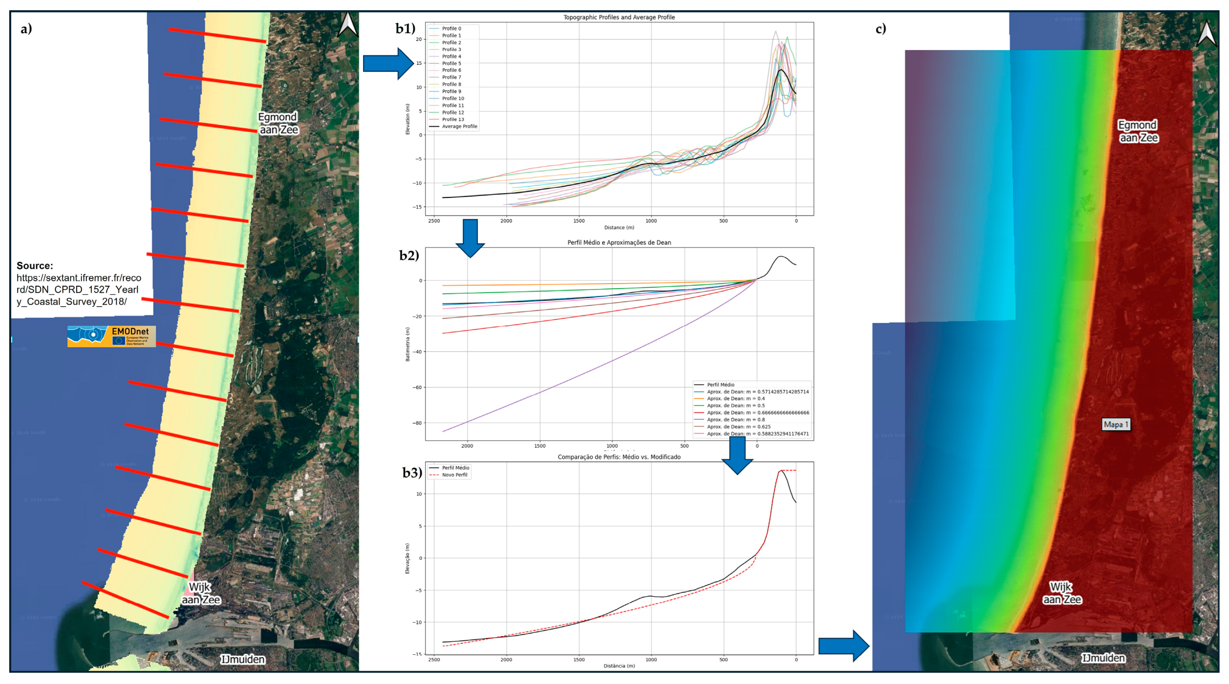
3.2.2. LTC Modelling—Setup

The study’s numerical domain for the coastal stretch in LTC was determined by analyzing the shoreline position using the digital elevation model provided by [48]. Based on the shoreline position, the bathymetry and topography of the coastal stretch were represented by a regular grid of points spaced 20 m apart in the west–east direction and 20 m apart in the north–south direction. This grid covered an area of 9.72 × 19.7 square kilometres (Figure 8).

The bathymetry was adjusted to match the shape of Dean’s profile, according to $h=A{x}^m$, based on EMODnet survey [48], and was considered regular and parallel along the coast. The topography was approximated using a constant slope of 4% (Figure 8(b2,b3)).

The wave climate used in the LTC model, as previously mentioned, consisted of the Measured-YM6 dataset and three reanalysis datasets: the ERA5 global model, and the offshore AENWS-WPR and the inshore AENWS-WPR North, both of which are regional models.

The reference scenario was established based on shorelines collected from aerial images, with the initial year being 1980 and the final year 2020. To extract the shoreline, the high-water line (HWL) methodology was applied, which relies on identifying the feature of the visibly distinguishable line on the wet beach–dry beach in the coastal imagery [49]. Using these shorelines, the areas of retreat and accretion were calculated, as well as the annual average shoreline retreat over the period. These values were used as reference points to evaluate the model calibration results.

For LTC model calibration, several configurations were tested, considering different artificial nourishment scenarios (200,000 m³/year, 250,000 m³/year, 300,000 m³/year, 400,000 m³/year, and 600,000 m³/year) and utilizing the Measured-YM6 wave dataset. Following an analysis of the results, three scenarios were identified as the most promising, based on the Measured-YM6 wave dataset: one scenario without artificial nourishment and two scenarios with artificial nourishment. The latter involved two areas and different sediment volumes—200,000 m³/year (A = 150,000 m³/year and B = 50,000 m³/year) and 250,000 m³/year (A = 150,000 m³/year and B = 100,000 m³/year). All scenarios considered the first year of simulation as the initial year of artificial sand nourishment, with a frequency of once per year. These scenarios were further simulated and analyzed using wave reanalysis datasets, as detailed in

Table 2. Scenarios’ design parameters modelled.

Dataset	Scenarios	Artificial Sand Nourishment
		Volume (×106 m3) Per Year	Total Volume (×106 m3)
S_Ref (real)—Aerial image coastline		-	-
Measured YM6 (Calibration)	S_YM6_200	0.20	8
	S_YM6_250	0.25	10
	S_YM6	-	-
ERA 5	S_ERA5_200	0.20	8
	S_ERA5_250	0.25	10
	S_ERA5	-	-
AENWS-WPR	S_AENWS_200	0.20	8
	S_AENWS_250	0.25	10
	S_AENWS	-	-
AENWS-WPR North	S_AENWS_N_200	0.20	8
	S_AENWS_N_250	0.25	10
	S_AENWS_N	-	-

.

The areas targeted for nourishment include a (A) 2500 m longshore stretch north of Wijk aan Zee and a (B) 2000 m section in the centre of study area (Figure 1). The nourishment covers the entire cross-shore active profile width up to 10 m in depth (considered the depth of closure), which is approximately 1400 m.

Sediment transport calculations were carried out using the CERC formula [44]. To calibrate the model, shoreline change rates were compared, assessing the mean shoreline retreat obtained numerically.

Regarding tidal forcing, the model incorporates tidal influence in two distinct ways: (i) maintaining the tidal level as a constant sea level throughout the entire simulation process, and (ii) allowing the tidal level to oscillate around the sea level throughout the entire simulation process. In the present simulation, the first option was chosen. The model validation was based on comparisons between the reference scenario (which includes areas and average annual retreat/accretion values, and the results obtained from the reference sediment transport (200,000–300,000 m³/year) and the results obtained from the LTC model considering the Measured-YM6 wave dataset. Additionally, artificial sand nourishment data (annual mean values) and input values from the calibration model were also considered.

4. Results

The numerical modelling results of shoreline evolution demonstrate that coastal nourishment contributes to reduce erosion in the study area over a 40-year simulation period, particularly in the locations defined in the model where the nourishments are performed.

The primary findings from the analysis of all the scenarios are presented and explored in this section, which begin with the discussion of the results for the reference scenario, followed by an evaluation of the performance of the several scenarios explored. In the conclusion, the key insights drawn from the obtained results are emphasized.

Reference Scenario

Figure 9 illustrates the evolution of the shoreline positions between 1980 and 2020, considering the reference scenario, based on the shoreline extraction from areal images (without modelling). The results highlight erosion in this period, particularly in two sectors, alternating with small sectors with accretion (Figure 9). Taking into account the timeframe 1980–2020 and all the shoreline extension of the study area, the annual average shoreline retreat is around 1 m/year. This corresponds to a territorial loss of approximately 81 hectares in 2020 (87.9 hectares of erosion and 6.9 hectares of accretion,

Table 3. Numerical modelling results of shoreline evolution in the study area, over a 40-year period, for the defined scenarios.

Dataset	Scenarios	Erosion (ha)	Accretion (ha)	Balance (ha)	Relative Error	Mean Retreat/Year (m)	Longshore Transport (m3/year)
S_Ref (real)		87.9	6.9	81.0	-	1.01	200,000–300,000
Measured YM6 (Calibration)	S 200,000 m3	90.4	14.3	76.1	−6.0%	0.95	231,250
	S 250,000 m3	90.2	18.0	72.2	−10.8%	0.90
	S without AN	95.1	7.8	87.3	7.8%	1.09
ERA 5	S 200,000 m3	89.3	15.8	73.5	−9.3%	0.92	180,696
	S 250,000 m3	89.0	19.4	69.6	−14.1%	0.87
	S without AN	94.6	9.9	84.7	4.6%	1.06
AENWS-WPR	S 200,000 m3	89.8	15.1	74.7	−7.8%	0.93	192,312
	S 250,000 m3	89.6	18.8	70.8	−12.5%	0.89
	S without AN	94.7	8.8	85.9	6.1%	1.07
AENWS-WPR North	S 200,000 m3	179.8	13.0	166.8	106.0%	2.08	115,511
	S 250,000 m3	179.5	16.8	162.7	101.0%	2.03
	S without AN	184.3	6.3	178.0	119.8%	2.23

Notes: Green—Correspond to accrection; Red—Correspond to erosion.

and Figure 10).

Regarding the LTC simulated scenarios, the parameters used to compare the deviations between the reference and the modelled scenarios were the longshore sediment transport volumes, which according to AX-COAST, 2023, is on average about 200,000–300,000 m³/year, the erosion–accretion area balance, and the mean shoreline retreat/year.

(a)

The 200,000 m³/year Nourishment Scenario

The analysis of the 200,000 m³/year (Figure 10(a1)) nourishment scenario reveals similar trends in erosion, accretion, and net balance. Erosion, represented by red bars, shows consistent levels across datasets, such as S_Ref, Measured-YM6, ERA5, and AENWS-WPR. However, a significant increase in erosion is observed in the AENWS-WPR North scenario, highlighting the sensitivity of these models to the wave-climate dataset. Accretion, depicted by blue bars, remains marginal across all datasets, indicating minimal sediment deposition regardless of the dataset employed. As expected from the erosion and accretion results, the net balance, represented by yellow bars, is similar for the first three datasets (Measured-YM6, ERA5, and AENWS-WPR), but exhibits a substantial increase in the AENWS-WPR North scenario.

The relationship between mean significant wave height (Hs) and balance area (ha) under these nourishment scenarios was also examined (Figure 10(a2)). The mean significant wave height varies between 0.9 m and 1.3 m across datasets. Scenarios with higher significant wave heights, Measured-YM6, AENWS-WPR, and ERA5, are associated with smaller balance areas, indicating a potential inverse relationship between significant wave height and sediment retention. The scenario AENWS-WPR North shows inverse behaviour that is probably related with the dataset’s main wave direction. Balance areas range from ≈74 ha to ≈170 ha. Lower balance areas, closer to ≈74 ha, are observed in the dataset ERA5, with significant wave heights (Hs = 1.2 m), reflecting more favourable conditions. In contrast, datasets like Measured-YM6 and AENWS-WPR report higher significant wave heights and balance areas close to 76 ha. AENWS-WPR North stands out with the smallest significant wave height (~0.95 m) and the highest lost balance area, exceeding 165 ha, suggesting that besides the significant wave height, other parameters, such as wave direction, have a relevant role in optimal sediment retention under lower wave energy.

The relationship between mean wave direction (Dir) in degrees and balance area (ha) further illustrates the dynamics of sediment redistribution (Figure 10(a3)). Wave directions range between 225° and 275° across datasets. AENWS-WPR North demonstrates the highest wave direction (~275°), while ERA5 reports the lowest (~225°). Lower wave directions (more oblique approaches) are associated with smaller loss areas (~74–75 ha), as seen in ERA5 and AENWS-WPR. Conversely, datasets with higher wave directions (more perpendicular approaches), such as Measured-YM6 (~235°) and AENWS-WPR North (~275°), achieve the highest loss areas, ~76 ha and ~170 ha, respectively. ERA5, AENWS-WPR, and Measured-YM6 show to be the most favourable, with their combination of high wave direction and low significant wave height indicating, in general, low loss balance area. In contrast, AENWS-WPR North struggles to maintain sediment stability under perpendicular wave approaches. This phenomenon occurs because the propagation of the waves to the coast by the LTC, which considers the Airy’s linear wave theory, may increase the percentage of waves coming perpendicular to the coastline. In addition, the AENWS-WPR dataset presents the mean wave direction predominantly from the west sector, making it more perpendicular to the coastline.

In synthesis, the inverse relationships identified between significant wave height, wave direction, and balance areas highlight critical dynamics in sediment redistribution. In general, lower significant wave heights and more oblique wave directions lead to reduced sediment-loss balance, emphasizing the importance of these factors in assessing coastal management strategies. The differences across datasets, particularly the consistent performance of ERA5, AENWS-WPR, and Measured-YM6 versus the challenges faced by AENWS-WPR North, underscore the variability in model responses to wave dynamics under nourishment conditions.

(b)

The 250,000 m³/year Nourishment Scenario

The 250,000 m³/year (Figure 10(b1)) nourishment scenario reveals similar erosion, accretion, and net-balance patterns across multiple datasets, when compared with the reference and the 200,000 m³/year scenarios. Accretion across all scenarios remains low, indicating limited sediment deposition effects despite the increased nourishment volume. However, the net balance was improved for all datasets when compared with the reference and the 200,000 m³/year scenarios. The AENWS-WPR North scenario demonstrates the highest sediment loss balance, likely due to an increase in erosion impacts and reduced sediment redistribution efficiency.

When comparing the 250,000 m³/year nourishment scenario to the 200,000 m³/year scenario, all datasets show a marked improvement in erosion, accretion, and net balance, indicating that higher nourishment rates may enhance coastal stability in regions represented by this model.

For the mean significant wave height vs. balance analysis (Figure 10(b2)), no significant changes are observed in this scenario, when compared with the 200,000 m³/year scenario. Interestingly, the increase in nourishment volume from 200,000 m³/year to 250,000 m³/year does not significantly impact the relationship between significant wave height and balance area. The overall trends and dataset-specific behaviours remain consistent, suggesting that additional sediment input has an influence on sediment retention in regions with high wave energy. The main finding is that, in general, increasing the artificial nourishment volume decreases the erosion rate and loss balance area, underscoring the importance of artificial nourishment in promoting favourable strategy against coastal erosion, in addition to the area and the surrounding area in which the nourishment is carried out.

Like for the significant wave height, the patterns found in wave direction versus balance area analysis (Figure 10(b3)) under the 250,000 m³/year nourishment scenarios mirror patterns observed in the 200,000 m³/year scenario. In this context, comparing wave-direction dynamics between the 200,000 m³/year and the 250,000 m³/year scenarios, the relationship between wave direction and balance area remains unchanged. For the increased nourishment volume, higher wave directions still lead to reduced sediment retention, particularly for datasets like AENWS-WPR North. This underscores the efficacy of additional sediment input in mitigating the negative impacts of perpendicular wave approaches.

(c)

Without Artificial Nourishment

In the absence of artificial nourishment (Figure 10(c1)), erosion levels are more significant across all dataset scenarios. The Measured-YM6 and AENWS-WPR scenarios in particular exhibit the highest erosion magnitudes, indicating a pronounced vulnerability to sediment loss under natural conditions. In contrast, accretion, which reflects sediment deposition, is minimal across all categories. This observation highlights the limited capacity for natural sediment deposition to counterbalance the erosive processes, irrespective of the dataset used. Consequently, the net balance is either low or negative across all scenarios, reflecting a sediment deficit. AENWS-WPR North demonstrates the worst performance compared to the other datasets, due to a highest relative difference between erosion and accretion.

The absence of nourishment leads to an increase in the net loss balance across all scenarios, underlining the role of artificial sediment input in mitigating coastal erosion. The erosion levels and negative balance across the Measured-YM6, ERA5, and AENWS-WPR datasets, between the with nourishment and without nourishment scenarios, are intensified.

Higher mean significant wave heights, such as those observed in Measured-YM6 and AENWS-WPR (>1.2 m), correspond to the highest loss balance areas (~87–86 ha, respectively), indicating significant sediment loss under high-energy conditions (Figure 10(c2)). Conversely, ERA5, with the lowest significant wave height (~1.2 m), achieves the lowest loss balance area (~85 ha), reflecting more favourable conditions for sediment retention. The S_Ref scenario report a loss balance area close to 81 ha. These results, although slightly higher than those observed in the nourishment scenarios, suggest that additional sediment transport processes, such as cross-shore transport, may be involved alongside longshore sediment transport.

Considering the mean wave direction vs. balance (Figure 10(c3)), like significant wave height, the patterns found in wave direction under the 250,000 m³/year nourishment and the 200,000 m³/year scenarios, the same tendency can be found in the scenarios without nourishment. In this context, comparing wave-direction dynamics between scenarios with nourishment and without nourishment, the relationship between wave direction and balance area remains unchanged. However, the areas obtained from the model are higher when compared with the reference scenario (S_Ref). The persistence of the relationship between wave direction and loss balance area, even without nourishment, emphasizes the critical role of hydrodynamic processes in sediment redistribution.

(d)

Analysis of Mean Retreat Under Different Nourishment Scenarios

The analysis of mean retreat rates (m/year) (Figure 10d) reveals a clear distinction between nourished and non-nourished scenarios. Without nourishment (W_out AN), retreat rates are consistently the highest across all datasets, with the AENWS-WPR North category exceeding 2 m/year, representing the most severe conditions. In contrast, nourishment scenarios (S 200 and S 250) demonstrate reduced retreat rates. However, the difference between the 200,000 m³/year (S 200) and 250,000 m³/year (S 250) scenarios is marginal, indicating that an increase in artificial nourishment may not represent proportional improvements in coastline stability or accretion.

By comparing the results from the Measured-YM6, ERA5, and AENWS-WPR datasets, it is evident that all exhibit similar trends and the same order of magnitude, highlighting the high quality of the reanalysis datasets. In contrast, AENWS-WPR North presents notably different values, as it represents an inshore wave reanalysis dataset. When incorporated into the LTC model, the model is again propagating the waves, which can further enhance wave direction, making it even more perpendicular to the coastline, in line with the wave linear theory.

(e)

Analysis of Relative Error Under Different Nourishment Scenarios

The analysis of relative error (%) (Figure 10e) offers insights into the predictive accuracy of the models under various nourishment scenarios. Measured-YM6, AENWS-WPR and ERA5 datasets demonstrate consistently low relative errors across all scenarios, indicating high alignment between modelled predictions and observed outcomes. The slight negative values suggest the positive influence of artificial nourishment. In stark contrast, AENWS-WPR North exhibits substantial overprediction, with relative errors exceeding 100% across all scenarios. This pattern suggests fundamental limitations in the scenario dataset.

The relative error in AENWS-WPR North remains consistent across the nourishment scenarios (S 200, S 250, and W_out AN), indicating that the error is dataset-dependent. In Measured-YM6, AENWS-WPR and ERA5, the 250,000 m³/year (S 250) scenario shows slightly higher negative errors compared to the 200,000 m³/year (S 200) scenario, reflecting the effect of an increase in nourishment volume. Without nourishment (W_out AN), relative error variations increase, indicating greater erosion, except in AENWS-WPR North, which continues to exhibit poor performance.

(f)

Impact of No Nourishment

The absence of nourishment increases the loss balance areas across all datasets. Scenarios with lower significant wave heights and directions, such as ERA5, demonstrate resilience even under natural conditions, while high-energy environments, as represented by Measured-YM6 and AENWS-WPR, face important challenges in maintaining sediment balance. These findings underscore the necessity of nourishment interventions to counteract the adverse effects of significant wave height and direction on sediment retention.

5. Discussion

Coastal erosion is a significant challenge within the study area, requiring a comprehensive understanding of sediment dynamics, including wave datasets, sediment erosion and accretion rates, and model calibration and validation. The proposed methodology was developed as part of the AX-COAST project, which aims to enhance the COAST tool—an innovative solution for cost–benefit analysis of coastal interventions [50]. COAST is an integrated tool for this type of evaluation, combining three modules: Coastal Evolution Module; Coastal Defense Structure Pre-Design Module; and Cost–Benefit Module [11,51,52,53].

Although this study does not focus on storm events, they play a crucial role in sediment dynamics, significantly altering erosion and accretion patterns compared to normal wave conditions. During storms, increased wave energy and surge levels drive intense sediment transport, often causing severe beach erosion and offshore sediment redistribution [21,22]. These events disrupt the equilibrium maintained by regular wave conditions, leading to rapid morphological changes that can persist long after the storm subsides. Conversely, post-storm recovery phases may involve localized sediment accretion due to longshore and cross-shore transport mechanisms [24,25].

The impact of storm events on sediment budgets underscores the importance of incorporating extreme weather conditions into numerical modelling to improve predictive accuracy and enhance coastal resilience strategies. By integrating storm-induced sediment transport processes into long-term models, coastal managers can better anticipate shoreline responses and design adaptive nourishment strategies to mitigate erosion risks.

As shown in Figure 5, the highest significant wave heights occur from September to March, predominantly from the SW-W direction, while from April to August, waves primarily come from the N-NNW direction, but with lower energy. This seasonal variability helps explain the erosion process, even with artificial sand nourishment. During winter, high wave energy removes sand from the beach, while in summer, the lower energy conditions do not allow sufficient time for natural sand recovery.

This study utilized four (4) wave datasets and artificial nourishment scenarios to explore diverse artificial nourishment options. A simple shoreline evolution model was applied to classify areas as lost, maintained, or gained, demonstrating the utility of simplified models in addressing the time and computational constraints of field data collection and three-dimensional modelling [51]. Nonetheless, gaps in long-term numerical modelling, particularly concerning artificial nourishments, require further research [54]. Addressing the long-term impacts of nourishment interventions on shoreline evolution is critical [9], as is incorporating short-term effects in long-term morphological modelling [55]. Additionally, limitations in field data, such as bathymetric, topographic, and long-wave data series, compounded by climate change uncertainties, remain substantial obstacles.

Regarding the 200,000 m³/year nourishment scenario highlights the AENWS-WPR North model as the most unfavourable, encountering pronounced erosion. In contrast, datasets like Measured-YM6, AENWS-WPR, and ERA5 exhibit lower variability, reflecting either relatively stable sedimentary dynamics or limitations in capturing localized sediment transport. This result indicates effective sediment management or better alignment with the region’s geomorphological characteristics. A strong inverse correlation between significant wave height and sediment retention is observed in these scenarios. As significant wave height increases, balance areas decrease, suggesting that elevated wave energy amplifies sediment erosion and redistribution, thereby diminishing retention. Among the datasets, ERA5 shows the most favourable conditions, characterized by lower significant wave heights and lower loss balance areas, making it particularly reliable for predicting sediment retention. Meanwhile, Measured-YM6 and AENWS-WPR highlight the challenges posed by higher significant wave heights, leading to increasing loss balance areas. Wave direction also emerges as a critical factor in sediment retention. Regarding wave directions, more oblique wave approaches, significantly reduce loss balance areas. ERA5 outperforms other datasets, with lower wave directions (more oblique approaches) correlating with lower balance areas. Conversely, AENWS-WPR North face difficulties maintaining sediment stability under these conditions, where higher wave directions (more perpendicular approaches) intensify erosive processes.

Under the 250,000 m³/year nourishment scenario, the AENWS-WPR North model continues to lead, demonstrating the lowest net sediment gain and underscoring its potential to intensify coastal erosion. Significant wave height remains a decisive factor in sediment retention, with higher waves consistently associated with highest loss balance areas. This reinforces the influence of hydrodynamic energy on sediment stability. ERA5 maintains its favourable performance, with lower significant wave height enabling lower loss balance areas. Wave direction continues to play a pivotal role. Oblique wave angles positively impact loss balance areas by driving alongshore sediment redistribution away from retention zones. ERA5, with its low wave directions, remains the most reliable scenario in this regard. However, the increased nourishment volume has limited impact on the wave direction–balance area relationship, suggesting diminished returns from higher sediment inputs, under specific conditions.

The absence of artificial nourishment underscores the critical role of sediment input in maintaining coastal stability. Without nourishment, net sediment balance decreases significantly across all datasets, with high-energy models such as Measured-YM6 and AENWS-WPR showing a more intense sediment loss. This disparity highlights the importance of nourishment interventions in stabilizing coastlines and mitigating erosive processes. Although increasing nourishment volumes from 200,000 m³/year to 250,000 m³/year reduces retreat rates modestly, the efficiency of these interventions decays as sediment volumes increase. ERA5 and AENWS-WPR exhibit robust performance, even in the absence of nourishment, with lower relative errors and higher loss balance areas, reflecting their resilience in dynamic environments. Conversely, AENWS-WPR North consistently overpredict sediment loss, struggling to maintain balance areas. Scenarios with lower significant wave heights, such as ERA5, achieve lower loss balance areas, further demonstrating their reliability under natural conditions. Wave direction plays a crucial role in the absence of nourishment. Oblique wave angles intensify sediment redistribution, further reducing balance areas in a more high-energy scenario. ERA5 continues to demonstrate resilience, maintaining lower loss balance areas with lower wave directions (more oblique approaches). Meanwhile, AENWS-WPR North face significant challenges in retaining sediment under perpendicular wave conditions.

As the authors of [9] demonstrate, the results highlight the critical influence of wave datasets on modelling outcomes, underlining the need for precise calibration to improve predictions. The results in [9] show, as the presented in this paper, that the nourishment impact is mainly observed nearby the intervention site. It is highlighted that higher longshore sediment transport rates are associated with more energetic wave climates, but not necessarily with incident waves more oblique to the shoreline.

Despite several challenges identified, artificial sand nourishment [11] has proven to be a valuable intervention. It effectively slows shoreline erosion, increases coastal economic value over time, and supports ecological conservation. Nourishment interventions maintain natural landscapes, enhance beach demand, promote economic and tourist activities, reduce coastal infrastructure maintenance costs, and minimize overtopping-related expenses [51]. During intense storms, these interventions reduce dune overtopping, contributing to broader storm resilience [56,57,58]. Expanded beach width further generates economic benefits [51,59,60,61].

6. Conclusions

This study evaluates coastal dynamics under different nourishment scenarios at IJmuiden, The Netherlands, assessing the effects of varying nourishment sediment volumes and the absence of nourishment using in situ and reanalysis wave-climate datasets (Measured-YM6, ERA5, AENWS-WPR, AENWS-WPR North).

Three scenarios of artificial nourishments were considered in the analysis: (1) considering a volume of 200,000 m³/year; (2) a volume of 250,000 m³/year; and (3) without nourishment. For the 200,000 m³/year scenario, model variability highlights the importance of localized observations in coastal management. Hydrodynamic forces play a crucial role, with lower significant wave heights (e.g., ERA5) improving sediment retention, while higher significant wave heights (e.g., Measured-YM6) reduce efficiency. Wave direction also influences retention, with more oblique approaches minimizing sediment losses.

The 250,000 m³/year scenario supports increased sediment volumes in specific contexts but shows that physical dynamics largely govern retention efficiency. ERA5 consistently delivers favourable results, reinforcing its reliability. Wave direction remains a key factor, with oblique angles reducing sediment loss.

Without nourishment, coastal systems face significant erosion, with sediment retention and balance areas diminishing across all models. ERA5 continues to perform well, underscoring the necessity of nourishment to stabilize coastlines and mitigate erosion.

These findings highlight the importance of scenario-specific methodologies and robust datasets in optimizing nourishment strategies. While increased nourishment can be beneficial, its effectiveness depends on dataset context. The study provides actionable insights for improving nourishment designs, model calibration, and long-term erosion management by evaluating wave-climate impacts and dataset differences.

References

1. Housley, J. Justification for Beach Nourishment. In Coastal Engineering 1996, Proceedings of the 25th International Conference on Coastal Engineering, Orlando, FL, USA, 2–6 September 1996; ASCE Libary: Orlando, FL, USA, 1996; p. 26. [Google Scholar]
2. Coelho, C. Riscos de Exposição de Frentes Urbanas Para Diferentes Intervenções de Defesa Costeira. PhD Thesis, University of Aveiro, Aveiro, Portugal, 2005. [Google Scholar]
3. Masselink, G.; Pattiaratchi, C.B. Seasonal Changes in Beach Morphology along the Sheltered Coastline of Perth, Western Australia. Mar. Geol. 2001, 172, 243–263. [Google Scholar] [CrossRef]
4. Hanson, H.; Brampton, A.; Capobianco, M.; Dette, H.H.; Hamm, L.; Laustrup, C.; Lechuga, A.; Spanhoff, R. Beach Nourishment Projects, Practices, and Objectives—A European Overview. Coast. Eng. 2002, 47, 81–111. [Google Scholar] [CrossRef]
5. Coelho, C.; Silva, R.; Veloso-Gomes, F.; Rodrigues, L. Artificial nourishment and sand by-passing in the aveiro inlet, portugal-numerical studies. Coast. Eng. Proc. 2011, 1, 99. [Google Scholar] [CrossRef]
6. Verhagen, H. Method for Artificial Beach Nourishment. In Coastal Engineering, Proceedings of the 23rd International Conference on Coastal Engineering, Venice, Italy, 4 October 1992; ASCE Libary: Orlando, FL, USA, 1992. [Google Scholar]
7. Tondello, M.; Ruol, P.; Sclavo, M.; Capobianco, M. Model Tests for Evaluating Beach Nourishment Performance. In Coastal Engineering, Proceedings of the 26th International Conference on Coastal Engineering, Copenhagen, Denmark, 22 June 1998; ASCE Libary: Orlando, FL, USA, 1998; Volume 3. [Google Scholar]
8. Marinho, B.; Coelho, C.; Larson, M.; Hanson, H. Short-and Long-Term Responses of Nourishments: Barra-Vagueira Coastal Stretch, Portugal. J. Coast. Conserv. 2018, 22, 475–489. [Google Scholar] [CrossRef]
9. Ferreira, A.M.; Coelho, C. Artificial Nourishments Effects on Longshore Sediments Transport. J. Mar. Sci. Eng. 2021, 9, 240. [Google Scholar] [CrossRef]
10. Davison, T.; Nicholls, R.; Leatherman, S. Beach Nourishment as a Coastal Management Tool: An Annotated Bibliography on Developments Associated with the Artificial Nourishment of Beaches. J. Coast. Res. 1992, 8, 984–1022. [Google Scholar]
11. Pais-Barbosa, J.; Ferreira, A.M.; Lima, M.; Filho, L.M.; Roebeling, P.; Coelho, C. Cost-Benefit Analysis of Artificial Nourishments: Discussion of Climate Change Adaptation Pathways at Ovar (Aveiro, Portugal). Ocean. Coast. Manag. 2023, 244, 106826. [Google Scholar] [CrossRef]
12. Camus, P.; Losada, I.J.; Izaguirre, C.; Espejo, A.; Menéndez, M.; Pérez, J. Statistical Wave Climate Projections for Coastal Impact Assessments. Earths Future 2017, 5, 918–933. [Google Scholar] [CrossRef]
13. Leake, J.; Wolf, J.; Lowe, J.; Stansby, P.; Jacoub, G.; Nicholls, R.; Mokrech, M.; Nicholson-Cole, S.; Walkden, M.; Watkinson, A.; et al. Predicted Wave Climate for the UK: Towards an Integrated Model of Coastal Impacts of Climate Change. In Estuarine and Coastal Modeling, Proceedings of the 10th International Conference on Estuarine and Coastal Modeling, Newport, RI, USA, 5 November 2007; American Society of Civil Engineers: Reston, VA, USA, 2008; pp. 393–406. [Google Scholar] [CrossRef]
14. Remya, P.G.; Kumar, R.; Basu, S.; Sarkar, A. Wave Hindcast Experiments in the Indian Ocean Using MIKE 21 SW Model. J. Earth Syst. Sci. 2012, 121, 385–392. [Google Scholar] [CrossRef]
15. Gómez-Orellana, A.M.; Fernández, J.C.; Dorado-Moreno, M.; Gutiérrez, P.A.; Hervás-Martínez, C. Building Suitable Datasets for Soft Computing and Machine Learning Techniques from Meteorological Data Integration: A Case Study for Predicting Significant Wave Height and Energy Flux. Energies 2021, 14, 468. [Google Scholar] [CrossRef]
16. Armenio, E.; De Serio, F.; Mossa, M.; Petrillo, A.F. Coastline Evolution Based on Statistical Analysis and Modeling. Nat. Hazards Earth Syst. Sci. 2019, 19, 1937–1953. [Google Scholar] [CrossRef]
17. Jaramillo, C.; Jara, M.S.; González, M.; Medina, R. A Shoreline Evolution Model Considering the Temporal Variability of the Beach Profile Sediment Volume (Sediment Gain/Loss). Coast. Eng. 2020, 156, 103612. [Google Scholar] [CrossRef]
18. Baptista, P.; Coelho, C.; Pereira, C.; Bernardes, C.; Veloso-Gomes, F. Beach Morphology and Shoreline Evolution: Monitoring and Modelling Medium-Term Responses (Portuguese NW Coast Study Site). Coast. Eng. 2014, 84, 23–37. [Google Scholar] [CrossRef]
19. Jara, M.S.; González, M.; Medina, R. Shoreline Evolution Model from a Dynamic Equilibrium Beach Profile. Coast. Eng. 2015, 99, 1–14. [Google Scholar] [CrossRef]
20. Subiyanto; Ahmad, M.F.; Mamat, M.; Husain, M.L. Comparison of Numerical Method for Forward and Backward Time Centered Space for Long-Term Simulation of Shoreline Evolution. Appl. Math. Sci. 2013, 7, 5165–5173. [Google Scholar] [CrossRef]
21. Simmons, J.A.; Splinter, K.D.; Harley, M.D.; Turner, I.L. Calibration Data Requirements for Modelling Subaerial Beach Storm Erosion. Coast. Eng. 2019, 152, 103507. [Google Scholar] [CrossRef]
22. Kim, T.-K.; Lim, C.; Lee, J.-L. Vulnerability Analysis of Episodic Beach Erosion by Applying Storm Wave Scenarios to a Shoreline Response Model. Front. Mar. Sci. 2021, 8, 759067. [Google Scholar] [CrossRef]
23. Li, F.; van Gelder, P.H.A.J.M.; Ranasinghe, R.; Callaghan, D.P.; Jongejan, R.B. Probabilistic Modelling of Extreme Storms along the Dutch Coast. Coast. Eng. 2014, 86, 1–13. [Google Scholar] [CrossRef]
24. de Winter, R.C.; Ruessink, B.G. Sensitivity Analysis of Climate Change Impacts on Dune Erosion: Case Study for the Dutch Holland Coast. Clim. Chang. 2017, 141, 685–701. [Google Scholar] [CrossRef]
25. Athanasiou, P.; van Dongeren, A.; Giardino, A.; Vousdoukas, M.; Antolinez, J.A.A.; Ranasinghe, R. Estimating Dune Erosion at the Regional Scale Using a Meta-Model Based on Neural Networks. Nat. Hazards Earth Syst. Sci. 2022, 22, 3897–3915. [Google Scholar] [CrossRef]
26. Vitousek, S.; Vos, K.; Splinter, K.D.; Erikson, L.; Barnard, P.L. A Model Integrating Satellite-Derived Shoreline Observations for Predicting Fine-Scale Shoreline Response to Waves and Sea-Level Rise Across Large Coastal Regions. J. Geophys. Res. Earth Surf. 2023, 128. [Google Scholar] [CrossRef]
27. Athanasiou, P.; van Dongeren, A.; Giardino, A.; Vousdoukas, M.; Antolinez, J.A.A.; Ranasinghe, R. A Clustering Approach for Predicting Dune Morphodynamic Response to Storms Using Typological Coastal Profiles: A Case Study at the Dutch Coast. Front. Mar. Sci. 2021, 8, 747754. [Google Scholar] [CrossRef]
28. Sembiring, L.; van Ormondt, M.; van Dongeren, A.; Roelvink, D. A Validation of an Operational Wave and Surge Prediction System for the Dutch Coast. Nat. Hazards Earth Syst. Sci. 2015, 15, 1231–1242. [Google Scholar] [CrossRef]
29. Hersbach, H.; Bell, B.; Berrisford, P.; Hirahara, S.; Horányi, A.; Muñoz-Sabater, J.; Nicolas, J.; Peubey, C.; Radu, R.; Schepers, D.; et al. The ERA5 Global Reanalysis. Q. J. R. Meteorol. Soc. 2020, 146, 1999–2049. [Google Scholar] [CrossRef]
30. Ministerie van Verkeer en Waterstaat. Kustnota, Traditie, Trends en Toekomst. Ministerie van Verkeer en Waterstaat; Ministerie van Verkeer en Waterstaat: The Hague, Netherlands, 2000. [Google Scholar]
31. Brand, E.; Ramaekers, G.; Lodder, Q. Dutch Experience with Sand Nourishments for Dynamic Coastline Conservation–An Operational Overview. Ocean. Coast. Manag. 2022, 217, 106008. [Google Scholar] [CrossRef]
32. Romão, F.; Coelho, C.; Lima, M.; Ásmundsson, H.; Myer, E.M. Cross-Shore Modeling Features: Calibration and Impacts of Wave Climate Uncertainties. J. Mar. Sci. Eng. 2024, 12, 760. [Google Scholar] [CrossRef]
33. Luijendijk, A.; De Vroeg, H.; Swinkels, C.; Walstra, D.-J. Coastal response on multiple scales: A pilot study on the ijmuiden port. In Proceedings of the Coastal Sediments, Miami, FL, USA, 2–6 May 2011; World Scientific Publishing Company: Singapore, 2011; pp. 602–615. [Google Scholar] [CrossRef]
34. Van Rijn, L. Improvement of Coastline Modelling Software Using Field Data. AX-COAST Report; AX-COAST: Aveiro, Portugal, 2023. [Google Scholar]
35. Stronkhorst, J.; Huisman, B.; Giardino, A.; Santinelli, G.; Santos, F.D. Sand Nourishment Strategies to Mitigate Coastal Erosion and Sea Level Rise at the Coasts of Holland (The Netherlands) and Aveiro (Portugal) in the 21st Century. Ocean. Coast. Manag. 2018, 156, 266–276. [Google Scholar] [CrossRef]
36. Vermas, T.; Boersen, S.; Wilmink, R.; Lodder, Q. National Analyses of Nourishments; Coastal State Indicators and Driving Forces for Bergen-Egmond, the Netherlands; Rijkswaterstaat and Deltares: Delft, The Netherlands, 2021. [Google Scholar]
37. Mummery, J.C. Available Data, Datasets and Derived Information to Support Coastal Hazard Assessment and Adaptation Planning. CoastAdapt Information Manual 3; National Climate Change Adaptation Research Facility: Gold Coast, Australia, 2016. [Google Scholar]
38. Hersbach, H.; Bell, B.; Berrisford, P.; Biavati, G.; Horányi, A.; Muñoz Sabater, J.; Nicolas, J.; Peubey, C.; Radu, R.; Rozum, I.; et al. ERA5 Hourly Data on Single Levels from 1940 to Present. Copernicus Climate Change Service (C3S) Climate Data Store (CDS). ERA 5. 2023. Available online: https://cds.climate.copernicus.eu/datasets/reanalysis-era5-single-levels?tab=overview (accessed on 31 July 2024).
39. Copernicus Marine Service Information. Atlantic- European Northwest Shelf- Wave Physics Reanalysis. E.U. Copernicus Marine Service Information (CMEMS). Marine Data Store (MDS). Available online: https://data.marine.copernicus.eu/product/NWSHELF_REANALYSIS_WAV_004_015/description (accessed on 31 July 2024).
40. Coelho, C.; Veloso-Gomes, F.; Silva, R. Shoreline Coastal Evolution Model: Two Portuguese Case Studies. In Coastal Engineering, Proceedings of the 30th International Conference, San Diego, CA, USA, 3–8 September 2006; McKee Smith, J., Ed.; World Scientific: San Diego, CA, USA, 2007; pp. 3430–3441. [Google Scholar]
41. Coelho, C.; Taveira Pinto, F.; Veloso Gomes, F.; Pais-Barbosa, J. Coastal Evolution and Coastal Works in the Southern Part of Aveiro Lagoon Inlet, Portugal. In Coastal Engineering, Proceedings of the 29th International Conference, National Civil Engineering Laboratory, Lisbon, Portugal, 19–24 September 2004; McKee Smith, J., Ed.; World Scientific: Lisbon, Portugal, 2004; pp. 19–24. [Google Scholar]
42. Lima, M.; Coelho, C. Improvement of an Existing Shoreline Evolution Numerical Model. In MARINE VIII: Proceedings of the VIII International Conference on Computational Methods in Marine Engineering, Göteborg, Sweden, 13–15 May 2019; CIMNE: Barcelona, Spain, 2019; pp. 502–513. [Google Scholar]
43. Lima, M.; Coelho, C. LTC Shoreline Evolution Model: Assumptions, Evolution, Validation and Application. J. Integr. Coast. Zone Manag. 2017, 17, 5–17. [Google Scholar]
44. CERC. Shore Protection Manual; U.S. Coastal Engineering Research Center: Washington, DC, USA, 1984; Volume 1. [Google Scholar]
45. Kamphuis, J.W. Alongshore sediment transport rate. J. Waterw. Port. Coast. Ocean. Eng.-ASCE 1991, 117, 624–640. [Google Scholar] [CrossRef]
46. Hanson, H.; Kraus, N.C. GENESIS: Generalized Model for Simulating Shoreline Chang—Report 1 Technical Reference, Technical Report CERC; Coastal Engineering Research Center, US Army Engineer Waterways Experiment Station: Vicksburg, MS, USA, 1991. [Google Scholar]
47. Silva, R. Avaliação Experimental e Numérica de Parâmetros Associados a Modelos de Evolução Da Linha de Costa. Ph.D. Thesis, Faculdade de Engenharia da Universidade do Porto, Porto, Portugal, 2010. [Google Scholar]
48. EMODnet. Available online: https://sextant.ifremer.fr/record/SDN_CPRD_1527_Yearly_Coastal_Survey_2018/ (accessed on 1 February 2024).
49. Boak, E.H.; Turner, I.L. Shoreline Definition and Detection: A Review. J. Coast. Res. 2005, 214, 688–703. [Google Scholar] [CrossRef]
50. Lima, M.; Coelho, C. COAST: Coastal Optimization Assessment Tool; Lima, M., Coelho, C., Eds.; UA Editora, Universidade de Aveiro: Aveiro, Portugal, 2024. [Google Scholar]
51. Coelho, C.; Lima, M.; Ferreira, M. A Cost–Benefit Approach to Discuss Artificial Nourishments to Mitigate Coastal Erosion. J. Mar. Sci. Eng. 2022, 10, 1906. [Google Scholar] [CrossRef]
52. Lima, M.; Ferreira, A.M.; Coelho, C. A Cost–Benefit Approach to Assess the Physical and Economic Feasibility of Sand Bypassing Systems. J. Mar. Sci. Eng. 2023, 11, 1829. [Google Scholar] [CrossRef]
53. Lima, M.; Coelho, C.; Veloso-Gomes, F.; Roebeling, P. An Integrated Physical and Cost-Benefit Approach to Assess Groins as a Coastal Erosion Mitigation Strategy. Coast. Eng. 2020, 156, 103614. [Google Scholar] [CrossRef]
54. Coelho, C.; Narra, P.; Marinho, B.; Lima, M. Coastal Management Software to Support the Decision-Makers to Mitigate Coastal Erosion. J. Mar. Sci. Eng. 2020, 8, 37. [Google Scholar] [CrossRef]
55. Larson, M.; Palalane, J.; Fredriksson, C.; Hanson, H. Simulating Cross-Shore Material Exchange at Decadal Scale. Theory and Model Component Validation. Coast. Eng. 2016, 116, 57–66. [Google Scholar] [CrossRef]
56. Itzkin, M.; Moore, L.J.; Ruggiero, P.; Hacker, S.D.; Biel, R.G. The Influence of Dune Aspect Ratio, Beach Width and Storm Characteristics on Dune Erosion for Managed and Unmanaged Beaches. Earth Surf. Dyn. 2020, 2020, 1–23. [Google Scholar]
57. Passeri, D.L.; Bilskie, M.V.; Hagen, S.C.; Mickey, R.C.; Dalyander, P.S.; Gonzalez, V.M. Assessing the Effectiveness of Nourishment in Decadal Barrier Island Morphological Resilience. Water 2021, 13, 944. [Google Scholar] [CrossRef]
58. Veloso-Gomes, F.; Costa, J.; Rodrigues, A.; Taveira-Pinto, F.; Pais-Barbosa, J.; Das Neves, L. Costa Da Caparica Artificial Sand Nourishment and Coastal Dynamics. J. Coast. Res. 2009, 1, 678–682. [Google Scholar]
59. de Schipper, M.A.; Ludka, B.C.; Raubenheimer, B.; Luijendijk, A.P.; Schlacher, T.A. Beach Nourishment Has Complex Implications for the Future of Sandy Shores. Nat. Rev. Earth Environ. 2020, 2, 70–84. [Google Scholar] [CrossRef]
60. Noordegraaf, I. Economic Valuation of Increased Beach Width at Praia Da Vagueira (central Portugal). Master’s Thesis, Wageningen University Netherlands, Wageningen, The Netherlands, 2020; 80p. [Google Scholar]
61. Raybould, M.; Mules, T. A Cost–Benefit Study of Protection of the Northern Beaches of Australia’s Gold Coast. Tour. Econ. 1999, 5, 121–139. [Google Scholar]
Figure 1. Study area, IJmuiden, The Netherlands.
Water 17 01091 g001
Figure 2. Converging and diverging tidal currents near IJmuiden harbour dams (Van Rijn, 1995, in [33]).
Water 17 01091 g002
Figure 3. A methodology to assess the shoreline behaviour using different wave datasets.
Water 17 01091 g003
Figure 4. A comparative analysis of the wave datasets (Measured-YM6, ERA5, AENWS-WPR and AENWS-WPR North) near IJmuiden.
Water 17 01091 g004
Figure 5. A comparative analysis of wave datasets by month (Measure-YM6, ERA5, AENWS-WPR and AENWS-WPR North), near IJmuiden.
Water 17 01091 g005
Figure 6. Forcing wave-data series (offshore and onshore wave parameters).
Water 17 01091 g006
Figure 7. Schematic representation of LTC model assumptions for cross-shore profile updates during computational calculations (adapted from [2]).
Water 17 01091 g007
Figure 8. (a) Bathymetry and topography provided by EMODnet; (b1) profiles extracted from EMODnet dataset; (b2) Dean’s profile bathymetry adjustment to the mean profile; (b3) Dean’s profile generation; and (c) bathymetry and topography generated for modelling.
Water 17 01091 g008
Figure 9. Coastline balance between 1980 and 2020. Reference scenario.
Water 17 01091 g009
Figure 10. LTC model results analysis for the simulated scenarios: (a1a3)—Scenario with 200,000 m³/year (S200) results; (b1b3)—Scenario with 250,000 m³/year (S500) results; (c1c3)—Scenario without artificial nourishment (W_out AN) results; (d)—Mean coastline retreat; (e)—Relative error for the considered scenarios.
Water 17 01091 g010aWater 17 01091 g010b