Investigating Steady-State Interpolation and Transient Hydraulic Modelling to Evaluate European Grayling Habitat in a Hydropeaking River

Abstract

Renewable energy sources such as hydropower are important to reduce the global emissions. Hydropower, however, comes with other environmental challenges by altering the ecological conditions in the rivers. Hydraulic models connected with fish habitat models could be one tool to assess the environmental impacts and evaluate mitigation measures for fish habitats. This study examines the limitations of steady-state hydraulic simulations in a low-sloping river located between two hydropower plants, where downstream regulations significantly influence the river flow dynamics. A 2D hydrodynamic model in Delft3D FM was applied to compare steady-state and transient simulations, focusing on how hydraulic variables affect the spawning habitat. The results show that steady-state models fail to capture time-dependent damping and delayed water level responses, leading to systematic underestimation of hydraulic variability. Peak bed shear stress values were under-predicted by the steady-state interpolation, which may under-predict spawning ground stability. Additionally, the steady-state approach failed to capture daily habitat fluctuations, resulting in a mean absolute error of 2910 m² in spawning habitat area per hour. This study demonstrates how errors in hydraulic calculations propagate into habitat assessments, potentially leading to misleading long-term evaluations of fish populations. This study highlights the importance of selecting appropriate hydraulic modelling approaches based on river-specific flow dynamics. Future studies should investigate the sensitivity of fish habitat models to hydraulic inputs from steady-state and transient simulations by integrating these approaches into advanced fish modelling tools, such as individual-based models. This will help determine the optimal balance between computational efficiency and accuracy in long-term habitat assessments.

1. Introduction

Hydropower has an important role in meeting electricity demands by providing a flexible and stable energy source in a power grid that includes more intermittent sources such as solar and wind power. However, hydropower infrastructure and operating schemes come with an environmental cost for the river ecosystem that prevents migrating fish to spawn in the river system, fish mortality caused by stranding [1,2], unsuitable flow conditions [3], and biodiversity losses [4]. According to the national plan for improving the ecological conditions in regulated rivers in Sweden, all hydropower facility environmental permits must be renewed [5]. Measures to improve the ecology in the river for each hydropower plant must be presented, where the goal is to fulfill the Swedish Environmental Code and the demand from the European Water Framework directive to achieve good ecological status (GES) for all watercourses [5]. Potential restoration measures may be both costly and time-consuming to investigate and implement, as they are often specific to the site and species involved, requiring individual assessments for each area. Hydraulic modelling connected with fish habitat models is one way to make these estimations more cost- and time-efficient.

A common factor among regulated rivers is that discharge management schemes significantly affect the hydraulic conditions in the river [6]. The frequency of regulation varies, with some rivers being adjusted more frequently to respond to fluctuations in electricity demand driven by energy markets. Operating schemes with rapid discharge fluctuations, also called hydropeaking events, have been studied for the potential effects on river dynamics and fish habitats [6]. Connecting the river dynamics with the complex behaviour of fish is important to understand the environmental pre-conditions and potential areas of improvement in the regulated river. Hydraulic conditions, morphological preconditions [1,7], food availability, temperature [8], oxygen level, predation, fish social behaviour during different flow conditions [9], and time during the day [1] are variables deciding the growth possibilities and ecological conditions for each fish species in the river. Capturing the dynamical behaviour of the river downstream the hydropower plant is important to understand how the discharge schemes affect the habitat areas over a given time period. Determining how the daily hydropeaking fluctuation impacts the river dynamics can give valuable information regarding hydraulic stages [6] and the potential spawning area [10]. The down- and up-ramping effects on stranding risks have also been studied [10,11], where water level alterations over time are used as a threshold, considering high or low risks of stranding fry and juvenile fish.

To understand the river dynamics and fish habitat as one, hydraulic data could be coupled with Individual-Based Models (IBM) to evaluate the long-term effects on different life stages of fish populations [12] under different flow regimes such as hydropeaking [13]. The flow conditions in the river are typically captured with an external hydraulic modelling software [14], and imported into the IBM, where they are used for environmental and biological analysis [15]. Using a hydraulic model to resolve the dynamic flow conditions in detail for the substantial time periods required for population-level modelling can be both data intensive and computationally expensive. Therefore, the depths and velocities can be simulated for different steady-state discharges, and they can be linearly interpolated to acquire intermediate velocities and depths under different flow conditions, which can then be combined in different ways to represent the flow conditions over a longer period of time [13,16,17]. This method requires several flow inputs to give a reliable result [16], but it is useful for evaluating new hydraulic conditions and operating schemes. However, steady-state interpolation assumes instantaneous equilibrium and does not account for storage effects, backwater influences, natural damping of the rivers, and response times, which can lead to errors in hydropeaking-affected rivers where hysteresis effects are present [18]. Although this approach is computationally efficient, it lacks the ability to capture short-term habitat fluctuations, potentially leading to habitat predictions that do not reflect the real ecological conditions.

Steady-state simulations are commonly used to estimate the hydraulic conditions in a river with different discharges [11,14,19]. In many cases, steady-state models are integrated into a habitat suitability index (HSI) model, which might introduce challenges in rivers regulated by hydropeaking operations. The simulations assume constant flow conditions where the discharge could either be averaged over days, months, or years, or it could be estimated to be a high peak or low flow. The discharge hydrographs for different up- and down-ramping events are also often assumed to go from a constant discharge to another constant state [10,20]. These types of simulations have shown good correlation during validation, since the interesting area is often a limited part of the river, and downstream boundaries can be placed far away from the interesting area so it does not effect the hydraulic results [20]. Using the energy slope as a boundary condition [21] or a constant water surface elevation [14] is a practical solution in scenarios where downstream regulation have minimal or no effects on upstream hydraulic conditions.

In some regulated rivers, both upstream and downstream hydropeaking operations influence hydraulic conditions, often resulting in decoupling between discharge and water levels. This means that a constant upstream discharge does not necessarily correspond to stable water levels, as downstream regulation can alter flow propagation via discharge release in the reservoir, which smooths out or delay changes in water levels. This can introduce variations where the assumptions of constant discharge and water level could lead to inaccurate predictions.

In hydropeaking rivers, key unresolved questions remain regarding how the temporal resolution of streamflow data and the spatio-temporal variation in flow depth, velocity, and wetted width influence environmental assessments [22]. Together with the non-stationary hydrological regimes driven by climate change and altered energy demand, the challenges with non-stable discharge water level relationships and capturing the correct time scale for the dynamic flow conditions [22] are important to resolve to assess the impact on the local scale of the river. Looking also at long-term fish habitats, the reservoir level in a hydropeaking river varies over the year, and therefore, hydraulic conditions for the same upstream discharge can differ. What applies during summer, when measurements for model calibration are often conducted, may not apply during spring or fall, when the river hydraulics are particularly influenced by downstream regulation or seasonal changes. This is a challenge when using steady-state interpolation, which assumes that water levels and velocities can be approximated from a set of simulated steady-state conditions. Although transient modeling is increasingly used in such cases, the high computational demands and uncertanties in defining realistic boundary conditions still make steady-state interpolation attractive for habitat assessments [23]. While steady-state interpolation is still commonly used in habitat models [13,16], its performance in hydropeaking rivers with regulation effects has been less explored [23].

This study critically evaluates whether steady-state interpolation can be a viable alternative in hydropeaking rivers with strong downstream influences. Additionally, this study examines whether steady-state simulations can be effectively used during periods of relatively stable reservoir water levels, while reserving transient simulations for periods of significant flow variation, such as spring floods, to capture essential questions connected to the time dependency of flow dynamics in hydropeaking rivers [22]. This hybrid approach could optimise computational resources while maintaining accuracy in habitat assessments. As part of a broader effort to connect hydraulic modelling with IBMs, this work serves as a first step in assessing the suitability of steady-state interpolation for this system. The analysis compares steady-state interpolation with a fully transient simulation, examining their performance in predicting hydraulic parameters relevant to habitat assessment. This study uses Delft3D FM Suite 2024.03 HMWQ for both transient and steady-state modelling, with MATLAB R2023b used for linear interpolation over time for the steady-state results. The findings provide practical insights into the limitations and benefits of steady-state interpolation, particularly in terms of flow dampening and downstream effects.

Study Area

The studied river is a regulated river in the northern part of Sweden, located between two hydropower plants, Akkats and Letsi. The distance between the upstream power plant and downstream dam is roughly 30 km. The 2D hydraulic model is limited to 15 km, measured from the outlet of the hydropower station upstream at the left corner in Figure 1. Further downstream, the hydraulic conditions are similar to a reservoir, so this area was excluded from the model in order to save computational time.

There was no comprehensive detailed bathymetry measurement over the entire river reach; rather, the bathymetry of the river is a combination of three digital elevation model (DEM) datasets, which all were provided by Vattenfall, AB. The height elevation data for floodplains and land area were provided by the Swedish land survey authority (Lantmäteriet). To combine the DEMs together, the geographic information system (GIS) tool ArcMap 10.8.2 was used with the reference system SWEREF 99 TM. This resulted in discontinuities in some overlapping areas, indicating that the datasets had measured the heights differently, even though they were extracted from same reference system. However, these discontinuities were small relative to the scale of the simulation domain and primarily affected localised areas rather than the overall hydraulic parameters. Since this study focuses on comparing modelling approaches rather than absolute accuracy, these errors are unlikely to significantly affect the comparative analysis.

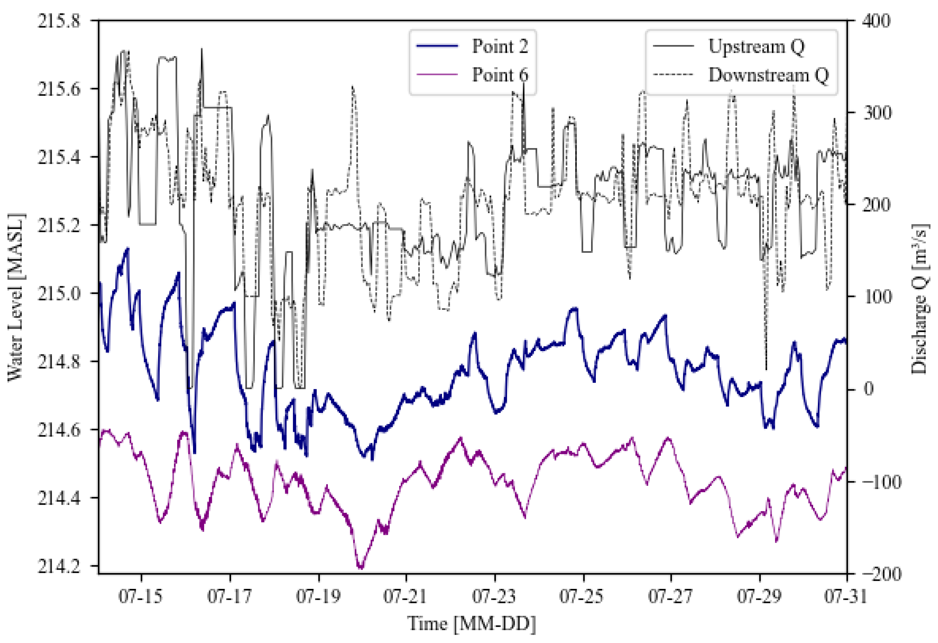
Previous work has been done in the river where the depth was measured from June–September 2021 with six pressure loggers together with an real-time kinematic (RTK) GPS pole to obtain the height elevation of the pressure loggers [24]. Combining the depth and elevation, the water surface elevation (WSE) can be obtained. The pressure logger locations are seen in Figure 1. The WSE from measurement points 2 and 6 is presented in Figure 2, with upstream and downstream discharge provided by Vattenfall, AB (Figure 2).

2. Numerical Modelling and Theory

2.1. Numerical Modelling

The 2D hydraulic model was developed in Delft3D FM. The model utilises a finite volume solver [25] and solves the Navier–Stokes equation under the Boussinesq and shallow-water assumptions. Hence, the velocities are depth-averaged [25]. The timestep in the model is automatically computed using the Courant criterion and was set to the default value of 0.7. The inlet boundary condition was set to the discharge from the upstream flow scheme. The outlet boundary condition was set to the measured WSE in point 6 to account for operational changes in discharge regulations downstream. In previous work [26], the Neumann water level gradient was tested as a boundary for the model, but without satisfying results. The walls were given a free slip condition, which is the default for a 2D model.

A steady-state solution does not take previous events into consideration, while a transient simulation considers the conditions from the previous time step. A steady-state simulation in the river is achieved by defining a constant discharge for the inlet boundary in the Delft3D FM model and a constant water level at the outlet boundary so that the hydraulic conditions are stagnated at an constant value. The steady-state simulations could then be used to linearly interpolate the hydraulic variables over time for different input hydrographs of discharge as follows:

$$WSE={\displaystyle \frac{WS{E}_1(Q_2-Q)+WS{E}_2(Q-Q_1)}{Q_2-Q_1}}$$

(1)

where $Q_1$ is the lower discharge, $Q_2$ the higher, Q is the requested discharge, and $WS{E}_{1,2}$ is the water surface elevation corresponding to each discharge. In the transient simulation, the model takes into account the hydraulic conditions of the previous time step. This is done by directly using the time-dependent hydrograph as an input for both the inlet and outlet instead of a constant discharge and water level. The solution is therefore time dependent. The hydrograph from Figure 2 was used to compare the methods.

As shown in the discharge graphs in Figure 2, similar flows from the upstream hydropower plant can result in different water levels, depending on the discharge at the downstream hydropower plant. This is clearly seen around 28–29th of June. To decide on how the steady-state cases should be chosen, two methods were tested. The first method was to average the WSE for each discharge value in the time period and divide it into groups as 0:50:400 m³/s to create a staircase graph (Figure 3a) where the most representative discharge of each group is plotted. The second approach was to find steady-state cases where the criterion was that the water level did not change during a period of 2 h and the discharge up- and downstream was held constant. Then, an average of the WSE in the groups was plotted to obtain the staircase graph in Figure 3b.

The second approach shows a more reasonable pattern than the first, with increasing WSE for increasing discharge. Seven steady-state cases were simulated in Delft3D FM using a constant input discharge with the corresponding water level from Figure 3b. The results were linearly interpolated (Equation (1)) to calculate the water surface elevations, depths, velocities, and bed shear stresses over time based on the hydrograph input from the discharge curve in Figure 2. The output of the transient simulation was directly extracted from Delft3D FM.

2.2. Response Time and Cross-Correlation

The response time was calculated with the cross-correlation function for time delays. The cross-correlation value decides how much one curve needs to be shifted, the lag, to be aligned with another. The cross-correlation between the two curves, discharge, and WSE, can be defined as follows:

$$R_{qy}\left(T\right)=\sum _{t}q\left(t\right)y(t+T)$$

(2)

where $q\left(t\right)$ is the normalised discharge time series, $y\left(t\right)$ is the normalised WSE, T is the lag (time or number of time steps) and $R_{qy}\left(T\right)$ is the cross-correlation value at lag T. To remove scale effects between the discharge and water level curves, normalization is done before calculating the cross-correlation. This is used to analyse the actual pattern in the signals rather than the absolute differences in their values. For the discharge,

$$q\left(t\right)={\displaystyle \frac{Q_t-Q_{min}}{Q_{max}-Q_{min}}}$$

(3)

and similar approach is used for the WSE. The response time is the position. The time lag where the cross-correlation reaches its maximum value is as follows:

$$T_{estimated} =arg\underset{T}{max}{R}_{qy}\left(T\right).$$

(4)

The response time was calculated for each element during the time period of 13–20 July with the MathWorks xcorr function [27]. The maximum response time was estimated from Figure 2 to 3 h, since delays larger than this are assumed to be related to downstream flow regulation and do not relate to the damping properties of the river.

2.3. Spawning Areas, Redds Scouring, and Stranding Risk

European grayling, which is a common fish species in the northern part of Sweden, could be more suitable as a restoration target than brown trout and salmon in regulated rivers, as they are less sensitive to impoundments [28] and show a larger variation in habitat preferences [29]. European grayling is the target species in this river, where the spawning areas are estimated from the velocity and depth preferences presented by Gönczi [30], with a wider span [24] than trout and salmon.

In rivers with frequent hydropeaking, stranding of fish is one factor of decreasing population growth of fish species caused by discharge magnitude, frequency, and ramping rates [31]. Stranding usually occurs after a high flow period followed by a rapid decrease in discharge and WSE, exposing especially younger life-stages with limited swimming abilities [32] such as larvae, frys and juveniles to dry conditions. In addition to discharge, down-ramping rates and time of the day have also been shown to have an impact on whether fish are stranded [1,10,31,33]. Most studies regarding fish stranding come from the alpine regions characterised by steep gradients [1,31,33,34]. However, the risk of fish stranding in low-sloping rivers should also be considered, since studies have shown that the magnitude of fish stranding is influenced by morphological characteristics such as slope [34], river bank [1], and substrate type [11,35], together with the magnitude of the baseflow [11]. Studies [36] have also shown that the lateral ramping rate, caused by the extent of dewatered area together with the magnitude of the baseflow, could also affect the risk of stranding, especially during down-ramping at low flow conditions [36]. This suggests that in low-sloping rivers, with low-sloping banks, where baseflow conditions can be more stable, sudden changes in flow can still lead to significant stranding risks caused by the lateral down-ramping rate rather than the vertical one [36].

The stranding risk is calculated by monitoring the water level over time in each element, discretised by the mesh in the hydraulic model, and determining if the WSE is the same value, or close to, the bed level, $z_{b_i}$. The time it takes for each element to reach the stranding threshold over one down-ramping event is identified by finding the minimum value, the first time step, that the threshold value is reached according to the following equation:

$$t_{dry}=min\{t:WS{E}_{i,t}\le z_{b_i}+0.05m\}.$$

(5)

were the threshold value is defined as 5 cm above the bed level. Then, the time step at the maximum WSE reached in the time series is identified so that the duration $\Delta t$ between the maximum WSE and the threshold can be calculated. The stranding velocity, the rate at which the water goes from its maximum level to the threshold, is then calculated as follows:

$$V_{stranding}={\displaystyle \frac{WS{E}_{max}-z_{b_i}+0.05}{\Delta t}}.$$

(6)

Together with stranding risk thresholds classified from studies [33] showing the highest WSE decrease over time that is allowed for different life stages and fish species, the stranding risk for a down-ramping event can be evaluated [10].

Scouring of redds (nests) is another consequence of high flows that can come from heavy rains and snow melting with the spring flood, and also from frequently high hydropeaking rivers [31,37]. Scouring of redds means that the gravel where the redds are buried is swept away and could be exposed to dryer conditions, leading to egg mortality from either long-term exposure or potential freezing [38,39]. Scouring of redds in dry reaches could also become a potential issue under modern hydropower operation strategies, where high spill events are increasingly influenced by electricity market prices rather than seasonal flow patterns. This shift may lead to more frequent and unpredictable spills compared to the historically lower and more consistent spill events. To interpret the scouring risk in a river, information about the flow conditions such as discharge, river morphology, and sediment transport are vital. Restoring spawning areas with suitable flow conditions in terms of depth and velocity could be non-efficient if the scouring risk of redds is too high. A restoration attempt aimed at improving the spawning habitat for European grayling in a regulated Swedish river showed no long-term effects on the grayling population [40], where the cause of this was not identified. Another restoration attempt for a regulated river in Northern Finland tagged and tracked graylings over 30-days [29]. The graylings stayed mostly in the restored area of the channel. Enhancing the restored area is preferable, providing them with a better habitat area, but no long-term effects were studied regarding population growth or the risk of transportation of the added spawning gravel.

The scouring risk can be estimated using sediment transport theory. In sediment transport, the Shields stress is usually used to predict sediment movement. It describes when the bed particles begin to move due to the force induced by the flow. The threshold of particle movement is given by the critical Shields stress:

$${\tau }_c^{*}={\displaystyle \frac{{\tau }_c}{({\rho }_s-{\rho }_w)gD}}$$

(7)

where ${\tau }_c^{*}$ is the Shields critical threshold derived from the Shields diagram, ${\tau }_c$ is the critical shear stress that is observed when particles begin to move, ${\rho }_s$ is the sediment density, ${\rho }_w$ is the water density, g is gravitational acceleration, and D is the mean particle diameter. The critical stress for motion depends on the specific flow conditions in the river, including depths and velocities. Larger particles are typically more stable and are primarily mobilised through bedload-induced motion, where transportation occurs through rolling, sliding, or saltation along the river bed. Therefore, factors such as bed slope, morphology, sediment mixture, and composition also matter in deciding the sediment movement and transportation in a river. To model bedload transportation, sediment transport models such as Meyer–Peter–Muller can be applied in Delft3D FM. In this study, the scouring risk is solely estimated using the critical shear stress for motion using the Shields threshold parameter. For gravel beds, the Shields critical threshold has been reported to be around 0.03–0.06 [41,42,43] depending on the flow conditions and particle sizes. Lower values are for particles that are easily mobilised, and higher values indicate more stability. To assess the potential for scouring, the bed shear stress simulated in Delft3D FM is compared with the critical shear stress. The depth-averaged bed shear stress in Delft3D FM is calculated as follows:

$${\tau }_b={\displaystyle \frac{{\rho }_{w}gU\left|U\right|}{C_{2D}^2}}$$

(8)

were $\left|U\right|$ is the magnitude of the depth-averaged horizontal velocity and $C_{2D}^2$ is the Chezy coefficient defined by the hydraulic radius R and Manning coefficient n:

$$C_{2D}={\displaystyle \frac{\sqrt[6]{R}}{n}}.$$

(9)

If the bed shear stress introduced by the flow conditions is higher than the critical shear stress, potential spawning gravel is assumed to be mobilised. Therefore, if any redds are buried in the gravel, the eggs within the redds may be displaced and could reduce the number of successfully emerged frys and decrease the long-term population. Long-term hydropeaking could impact the river morphology by removing gravel from potential spawning habitats, making them non-usable for the fish even though the flow conditions are good. Preferable spawning gravel for European graylings have been reported to be coarse gravel (8–16 mm), fine pebbles (16–32 mm), and coarse pebbles (32–64 mm) [44], with variations of up to 256 mm [29], giving a wide range but with a preferable size of 16–32 mm [44].

3. Mesh Study and Calibration

The domain is discretised with a flexible mesh in the mesh module RGFGRID in Delft3D FM. The grid is built up of rectangular elements in the main channel and triangular elements in areas peripheral to the main channel [26]. The approach has been discussed in various studies [45,46], where flexible meshes have been shown to give good results and be computationally efficient. Key mesh properties such as aspect ratio and orthogonality are critical for resolving the equations properly. The recommended aspect ratio is between 1:2 and 1:4, so the length of each cell should not exceed four times its width [25], with an optimal value of around 1:3. The orthogonality should ideally remain below 0.02 in the interesting areas [25], and it was kept below 0.02. The transition between triangular cells should maintain smoothness between 10 and 20%, although some shoreline regions showed values as high as 40–80%. Another important property of the mesh is that it is fine enough to resolve an accurate bed elevation. The mesh’s capacity to discretise the bathymetry properties could have a larger impact than the numerical diffusion from mesh properties such as orientation, size, and form [46]. The bathymetry had a resolution of 2 × 2 m, and the model domain spans over 15 km, with a maximum width of 900 m. This makes it computationally expensive to have a very fine mesh. Five mesh sizes were modeled, where the finest mesh in the study had an average cell size of 4.86 × 2.44 m (

Table 1. Statistics for the grids.

Statistic	Mesh 1	Mesh 2	Mesh 3	Mesh 4	Mesh 5
Grid Elements	10,000	40,000	160,000	360,000	640,000
M-Size (MAX/AVE)	82.4/38.9	42.2/19.4	16.5/14.5	14.2/6.5	10.7/4.86
N-Size (MAX/AVE)	38.2/18.7	20.3/9.7	10.3/4.5	6.9/3.3	5.15/2.44

). The Froude numbers using this mesh for the highest flow in Figure 2 were above the supercritical limit for 0.2% of the elements and below 0.2 for 73%. In total, 77% of the elements had a defined water depth and Froude number. The high Froude numbers were located close to the inlet, indicating that a fine resolution is necessary to capture the flow changes and transition zones in this region.

Four cross sections were chosen for the mesh studies: one across an island, one with triangular/curvilinear transition, one upstream at the widest part in the channel, and one in the most narrow part (Figure 1). The bed level was resolved in ArcMap and then compared to the bed level variable in Delft3D FM (

Table 2. Mean Absolute Error (MAE) and maximum error of the bed level for different meshes across various cross sections. Measured bathymetry is reference.

Bed Level [m]		CS Island		CS1		CS2		CS3
Mesh	Time [h]	MAE	Max Error	MAE	Max Error	MAE	Max Error	MAE	Max Error	AVE Error
Mesh 1	0.05	0.41	2.55	0.46	2.61	0.73	3.74	0.74	4.75	0.59
Mesh 2	0.14	0.19	1.55	0.24	1.68	0.49	3.46	0.40	3.32	0.33
Mesh 3	0.42	0.11	1.31	0.12	1.55	0.28	2.08	0.30	2.50	0.20
Mesh 4	1.15	0.09	1.28	0.09	1.53	0.20	1.53	0.24	2.29	0.16
Mesh 5	3.84	0.06	1.26	0.06	0.66	0.17	1.64	0.21	1.96	0.13

). The average mean error across all cross sections for the finest mesh was 0.13 m, with an maximum error of 1.96 m. The finest mesh had an overall good agreement with the bathymetry, except for some large outliers. The simulation time for Mesh 5 was around three times higher than for Mesh 4.

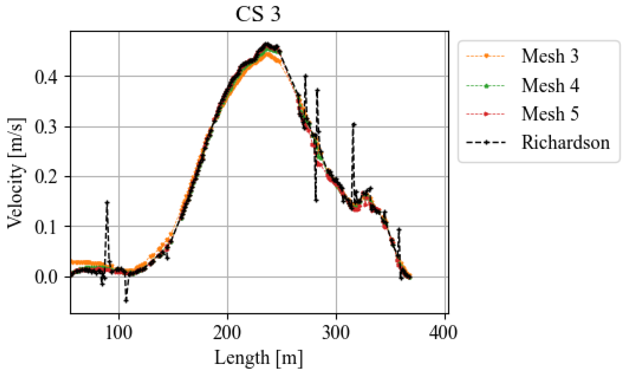
The depth and velocity were chosen as hydraulic parameters to investigate. The depth was compared with the finest mesh, where the depth for Mesh 4 had an average error of 0.05 m and a maximum of 1.16 m (

Table 3. Mean Absolute Error (MAE) and maximum error of depth for different meshes across various cross sections. Mesh 5 is the reference.

Depth [m]	CS Island		CS1		CS2		CS3
Mesh	MAE	Max Error	MAE	Max Error	MAE	Max Error	MAE	Max Error	AVE Error
Mesh 1	0.26	1.69	0.34	1.77	0.53	3.53	0.52	4.13	0.41
Mesh 2	0.10	1.25	0.13	1.32	0.28	3.17	0.22	2.19	0.18
Mesh 3	0.04	1.00	0.04	1.12	0.11	1.38	0.13	1.04	0.08
Mesh 4	0.02	0.84	0.03	0.70	0.07	0.61	0.09	1.16	0.05

). The convergence in velocity was calculated based on Richardson’s Extrapolation [47] (Figure 4).

The Richardson extrapolation (Figure 4) showed some oscillations when the error between two meshes changed sign. This approach assumes a convergence towards a larger or smaller value, and when one mesh suddenly changes sign or overlaps with the other, this lead to oscillatory convergence [47]. A filter approach was used to minimise the spikes in the results by applying a mask before the calculation to remove division by zero or very small values, and another mask was applied to remove unwanted patterns (e32/e21 < 0) that could lead to oscillations [47]. The velocity was differing most at cross section CS1, with −3.2% for the finest mesh and −4.2% for the second finest mesh (

Table 4. Maximum values and percentage errors of velocity for different meshes across various cross sections with Richardson extrapolation.

Velocity [m/s]	CS Island		CS1		CS2		CS3
Mesh 1	0.35	$+10.8\%$	0.43	$-15.9\%$	0.10	$-9.5\%$	0.41	$-11.5\%$
Mesh 2	0.29	$-7.2\%$	0.48	$-6.5\%$	0.10	$-7.2\%$	0.42	$-10.0\%$
Mesh 3	0.31	$-2.1\%$	0.48	$-5.5\%$	0.11	$-2.7\%$	0.44	$-4.6\%$
Mesh 4	0.32	$-0.1\%$	0.49	$-4.2\%$	0.11	$-0.6\%$	0.46	$-1.5\%$
Mesh 5	0.32	$-0.0\%$	0.49	$-3.2\%$	0.11	$-0.1\%$	0.46	$-0.5\%$
Richardson	0.32		0.51		0.11		0.47

).

Based on the result of the bed-level resolution, computational efficiency, depth, and velocity convergence, Mesh 4 was chosen to resolve the river domain.

The roughness of the bed level was chosen as the calibration parameter. A series of steady-state simulations were performed with a uniform roughness value, varying between 0.01 and 0.10 in increments of 0.01. The simulations were performed with a constant flow rate of 234 m³/s and 316 m³/s. These were chosen from the measurements on 11 August and 12 July. The peaks were smoothed over 3 h to approximate steady-state cases. The WSE results from each simulation were compared against six measurement points along the reach. The roughness value that produced the best agreement with the observed WSE at each measurement point was then selected and specified to the area centered around the measurement point. This resulted in a spatially varying roughness distribution where the computational domain was divided into six parts centered around each measuring point. The final roughness values and the differences in water levels from the measurements are shown in

Table 5. Calibrated roughness coefficients and the height difference between measured and simulated water levels. Negative values indicate that the model underestimates the water level.

Area	1		2		3		4		5		6
Roughness n	n	[m]	n	[m]	n	[m]	n	[m]	n	[m]	n	[m]
234 m3/s	0.01	0.06	0.07	0.03	0.05	0.01	0.08	$-0.01$	0.07	0.01	0.06	0.00
316 m3/s	0.01	$-0.01$	0.06	0.01	0.05	0.02	0.07	$-0.02$	0.06	$-0.01$	0.03	0.00
Final roughness	0.01		0.065		0.05		0.07		0.065		0.045

.

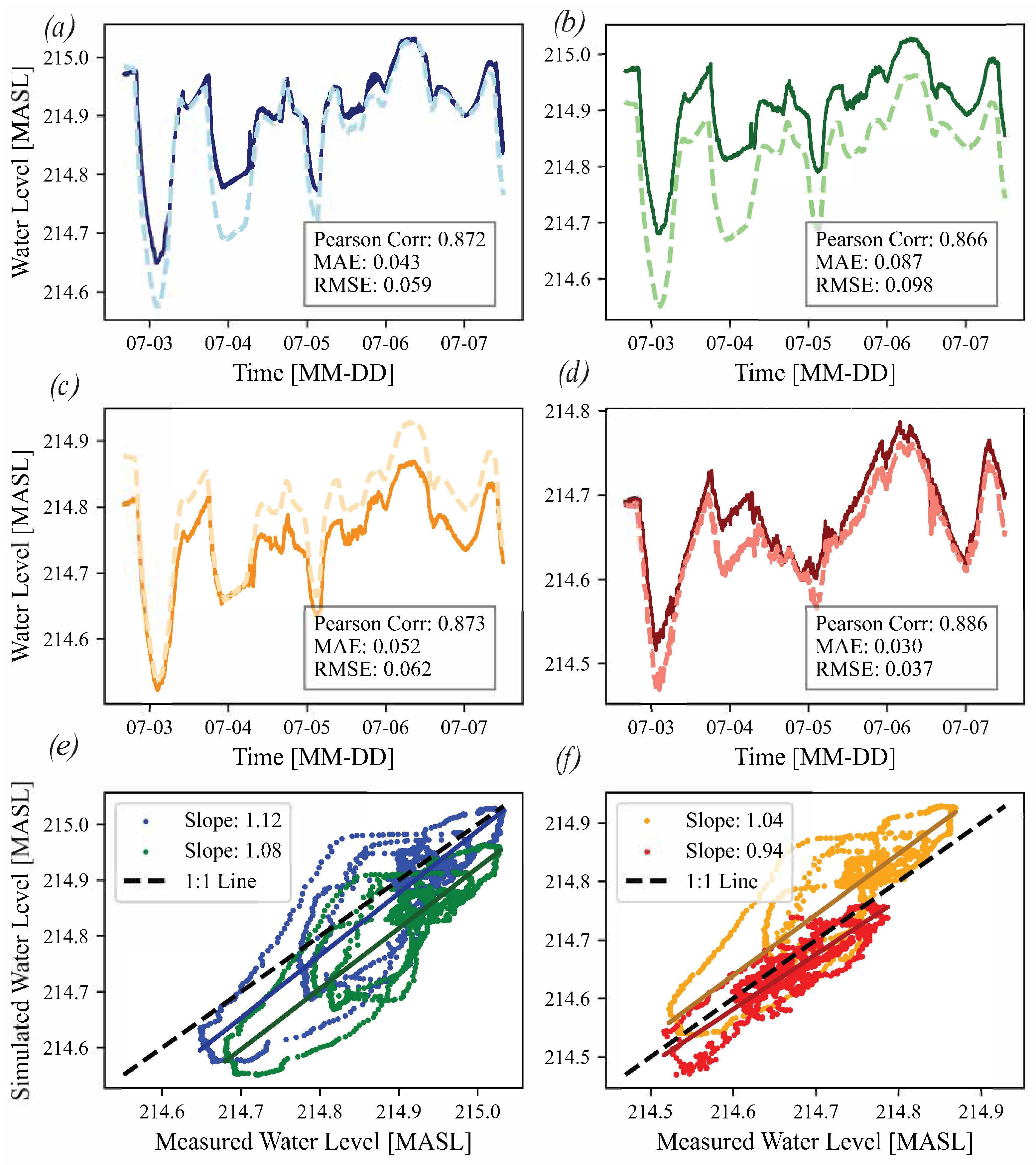
The roughness values for the two cases are quite similar. The mean value between the two flows was chosen, and the roughness was linearly increased or decreased between the computational domains. With the calibrated roughness, the model was simulated between 2 and 7 July to evaluate its performance. The simulated and measured water levels were compared at four points, as shown in Figure 5a–d. Figure 5e,f, which include scatterplots illustrating the measured values fitted against the simulated values over time.

The relatively high Pearson correlation coefficient demonstrates that the model captures the patterns of water level changes over time. The highest mean absolute error (MAE) was 0.087 m for Point 3, and the lowest was 0.03 m for Point 5. The root mean square error (RMSE) takes into consideration the high peaks in differences more than the MAE, where a high RMSE indicates that the errors are more spread out from the mean. A lower RMSE suggest that the model predictions are not generally accurate but also do not have significant outliers or large errors. The RMSE was highest for Point 3, which is expected because of the high MAE and low Pearson correlation. With the help of Python 3.12 Numpy module polyfit, the slope and interception were calculated, and together with polyval, a fitted line was plotted. The slope of the line defines the increase and decrease rate of the simulated and observed water level. A slope of one means that for every increase in observed water level, the simulated level increases by the same amount, giving perfect agreement. At point 2 (Figure 5a), which presents the highest slope, the model underpredicts water levels at the lower end but provides rather accurate estimates at higher water levels. In contrast, at point 3 (Figure 5c), the model systematically overpredicts the water levels, though its predictions are more accurate at the lower water levels. The model captures the trends based on the Pearson correlation and has a maximum MAE of 0.087 m and a minimum of 0.03 m. There are, however, systematic errors when looking at the slopes, which indicates that the model is either too fast in responding to the changes in water levels (slope > 1) or too conservative (slope < 1). The model overall predicts the water levels at an acceptable level for the purpose of this study.

4. Results

4.1. Response Time and Stranding Risk

The WSE was extracted upstream at measurement Point 2 to obtain the WSE response near the outlet of the hydropower station and downstream at Point 5 to investigate differences between the upstream and downstream responses. At measurement Point 2, the WSE response in the transient simulation and the steady-state interpolated curve showed similar patterns (Figure 6). While some differences were observed, the steady-state interpolated curve generally captured the short-term changes in WSE. The mean absolute error (MAE) was 0.088 m, and the maximum absolute error was 0.40 m.

Further downstream at measurement Point 5 (Figure 7), greater deviations in the pattern can be seen between the transient simulation and the steady-state interpolation. The MAE between the curves was 0.088 m, similar to point 2, and the maximum absolute error was only 0.31 m. The difference between the methods can be explained by the neglect of backwater effects and loss of dampening in the steady-state approach. Since the steady-state interpolation assumes an immediate response between the defined discharge conditions, it fails to capture the progressive change in water level variations that occur in the dynamical flow. Furthermore, downstream regulation influences the WSE, and the steady-state approach does not always capture how these effects alter the water levels. In contrast, the transient simulation models these unsteady flow processes, leading to a more accurate representation of downstream WSE over time.

The differences between the two methods can be furthered explained by looking at the response time. For the first method, it is uniform over the whole river (Figure 8a), as the steady state interpolation between time steps does not take into consideration the damping properties of the river. For the transient simulation (Figure 8b), the response time varies across the whole river and increases with the distance from the outlet of the hydropower station.

For the downstream section, the response time was harder to estimate due to the dependency of the downstream hydropower station, and a maximum lag of 3 h was set. The cross-sectional longitudinal curve (Figure 9a) shows that the maximum response time was reached after around 9 km.

The stranding risk for European grayling can be calculated by looking at the changes in WSE over time. The stranding risk was estimated from the highest flow change during 15–16 July and was calculated with the stranding velocity, which was categorised into five different statuses [10,33]. All elements that fulfilled the criteria in Equation (5) are shown in Figure 9b,c. Lower element indices correspond to locations near the hydropower outlet, while higher element indices are situated closer to the reservoir.

The stranding risk for the interpolated steady-state estimation is higher upstream and also propagates further downstream than for the transient simulation. This can be explained by the fast response times of the steady-state interpolation. This means that the down-ramping time for each element across the river will be exactly the same, while the depth changes are different, causing the different stranding velocities. The fast response also causes elements in the upstream part to have higher stranding risk because of the larger changes in WSE. Downstream, the variation is lower, which can be seen in the WSE curves in Figure 6 and Figure 7, causing the lower stranding velocities.

4.2. Hydraulic Variables and Spawning Areas

The depth and velocity was compared by extracting the variables on 19 July, when the water levels were lowest during the time period. There was a significant difference between the two simulation methods. The values were extracted at the cross section located furthest downstream in Figure 1, which is the most narrow section of the river reach downstream. The maximum depth difference in the chosen time step and cross section was 0.15 m, and the velocity difference was 0.06 m/s (Figure 10). The velocity and depth across all elements and time steps were used to find spawning areas according to the preferred depths and velocities of European grayling [24,30]. The total spawning area observed over time is presented in Figure 11. The spawning area differs over time, where the interpolated steady-state fails to show the variation that occurs daily.

The spawning area varies over time, where the interpolated steady-state approach fails to capture the daily fluctuations. The steady-state fails to capture the spawning area, with a MAE of 2910 m² per hour. To analyse the daily variations that arise from using different methods, the areas where velocity and depth conditions meet the spawning criteria are presented alongside the total spawning area in Figure 12. This comparison is shown for two scenarios, one influenced by downstream regulation and one during a downramping event at the upstream hydropower plant.

In the first scenario (Figure 12a), the discharge from the upstream hydropower plant remains constant, but due to downstream regulation, the available area meeting the depth criterion differs by 52.9% compared to the steady-state interpolation. At the same time step, the available velocity area differs by 1.63%, while the total spawning habitat area differs by 32.2%. This indicates that depth variation is the primary factor contributing to deviations between the methods. The downstream regulation, and consequently the backwater effect, is a process that the steady-state interpolation fails to capture, leading to significant differences in estimated habitat availability. In the second scenario (Figure 12b), the primary factor influencing differences in estimated spawning habitat is the velocity. In this case, a down-ramping event occurs at the upstream hydropower plant, where discharge decreases from 230 m³/s to 130 m³/s between 00:00 and 01:00, while downstream regulation remains relatively constant. At 01:00, the difference in depth is 0.69%, the difference in velocity is 38.8%, and the difference in the spawning area 21.9%. The steady-state interpolation, which responds instantaneously to discharge changes, overestimates the available area meeting the velocity criterion. In contrast, the transient simulation captures the gradual adjustment of flow conditions, leading to a more accurate estimation of spawning habitat availability. The hourly mean absolute error in estimated spawning habitat for these two scenarios is 5619 m² and 2614 m², respectively.

4.3. Bed Shear Stress and Redds Scouring

The scouring risk for redds in the river is estimated using the Shields critical threshold for motion with the characteristic flow conditions of the spawning areas. The gravel size suitable for grayling spawning was set to 16–64 mm [44], with depth ranges of 0.3–1.1 m and velocities of 0.2–0.9 m/s. The density of gravel is assumed to be 2650 kg/m³, which is common to use in sediment transport theory [48,49]. The Shields critical threshold for motion was divided into three categories, estimated to be 0.03 for easily mobilised particles and 0.045 for more stable particles, as previously reported in the literature for gravel bed streams [43]. The critical shear stresses for the lower and upper limit were calculated using Equation (7) and are shown in

Table 6. Critical bed shear stress for spawning gravel sizes: fine (16–32 mm) and coarse (32–64 mm) pebbles.

Gravel Size (mm)	No Risk	Potential Risk	High Risk
	(${\mathbf{\tau }}_{\mathbf{c}}^{*}\le \mathbf{0}.\mathbf{03}$)	($\mathbf{0}.\mathbf{03}<{\mathbf{\tau }}_{\mathbf{c}}^{*}<\mathbf{0}.\mathbf{045}$)	(${\mathbf{\tau }}_{\mathbf{c}}^{*}\ge \mathbf{0}.\mathbf{045}$)
16 mm	${\tau }_c\le 8{\mathrm{N}/\mathrm{m}}^2$	$8{\mathrm{N}/\mathrm{m}}^2<{\tau }_c<12{\mathrm{N}/\mathrm{m}}^2$	${\tau }_c\ge 12{\mathrm{N}/\mathrm{m}}^2$
32 mm	${\tau }_c\le 16{\mathrm{N}/\mathrm{m}}^2$	$16{\mathrm{N}/\mathrm{m}}^2<{\tau }_c<24{\mathrm{N}/\mathrm{m}}^2$	${\tau }_c\ge 24{\mathrm{N}/\mathrm{m}}^2$
64 mm	${\tau }_c\le 31{\mathrm{N}/\mathrm{m}}^2$	$31{\mathrm{N}/\mathrm{m}}^2<{\tau }_c<47{\mathrm{N}/\mathrm{m}}^2$	${\tau }_c\ge 47{\mathrm{N}/\mathrm{m}}^2$

.

The bed shear stress for both the transient and steady-state simulations were estimated using Equations (8) and (9). The differences between the methods include how the bed shear stress is obtained over time. In the steady-state approach, the bed shear stress is linearly interpolated from the seven uniform flow cases to estimate its variation over time. In contrast, the transient simulation directly calculates the bed shear stress at each time step based on the time-dependent velocity and hydraulic radius, capturing real-time variations for the dynamic flow. The bed shear stress was plotted for one element over time (Figure 13a) in a spawning area upstream, close to the outlet of the hydropower plant, and for a longitudinal cross section (Figure 13b) following the main stream to display differences in up- and downstream estimations.

The steady-state interpolated estimation is missing peaks in bed shear stress in the upstream part of the river. Downstream, the steady-state is overestimating it. After 8 km, the amplitude of the bed shear stress is overestimated, similar to the damping properties that the steady-state simulation neglects. Both transient and steady-state interpolation curves show high risk of scouring of redds of fine pebbles in the upstream part, while the steady state shows high risk both up- and downstream. Compared with the upper limit of the coarse pebbles in Table 6, the steady-state interpolation curve misses the high peaks and has only a potential risk, while the transient simulation shows a high risk of scouring.

5. Discussion

The aim of this study was to investigate the differences between a transient and steady-state approach to estimate the dynamic flow conditions of a regulated river. The performance of the hydraulic model was considered accurate enough for this purpose. One thing that could affect the accuracy of the model was the combination of the DEMs of different resolutions. Two high-resolution DEMs (0.25 × 0.25 m) and one lower-resolution DEM (2 × 2 m) were combined. There were differences in the DEMs when comparing the height elevations in several points with an average difference of 1 m. Interpolating these DEMs likely impacts the accuracy of habitat modelling, especially when considering depths. However, since this study focuses on comparing methods, these errors are unlikely to affect the analytical results significantly. To improve the model’s accuracy, it would be preferable to obtain a detailed DEM for the entire river reach.

During the calibration process, increasing the roughness in section 3 led to only minimal improvement at measurement Point 3, while it increased the error at Point 2. The model both under- and overestimates the WSE when the differences in WSE can also be related to uncertainties in the measurements. According to the recorded RTK GPS positions at the beginning and end of the field measurements, at Points 3 and 4, the pressure loggers were displaced, causing variations in height of around ±0.1 m.

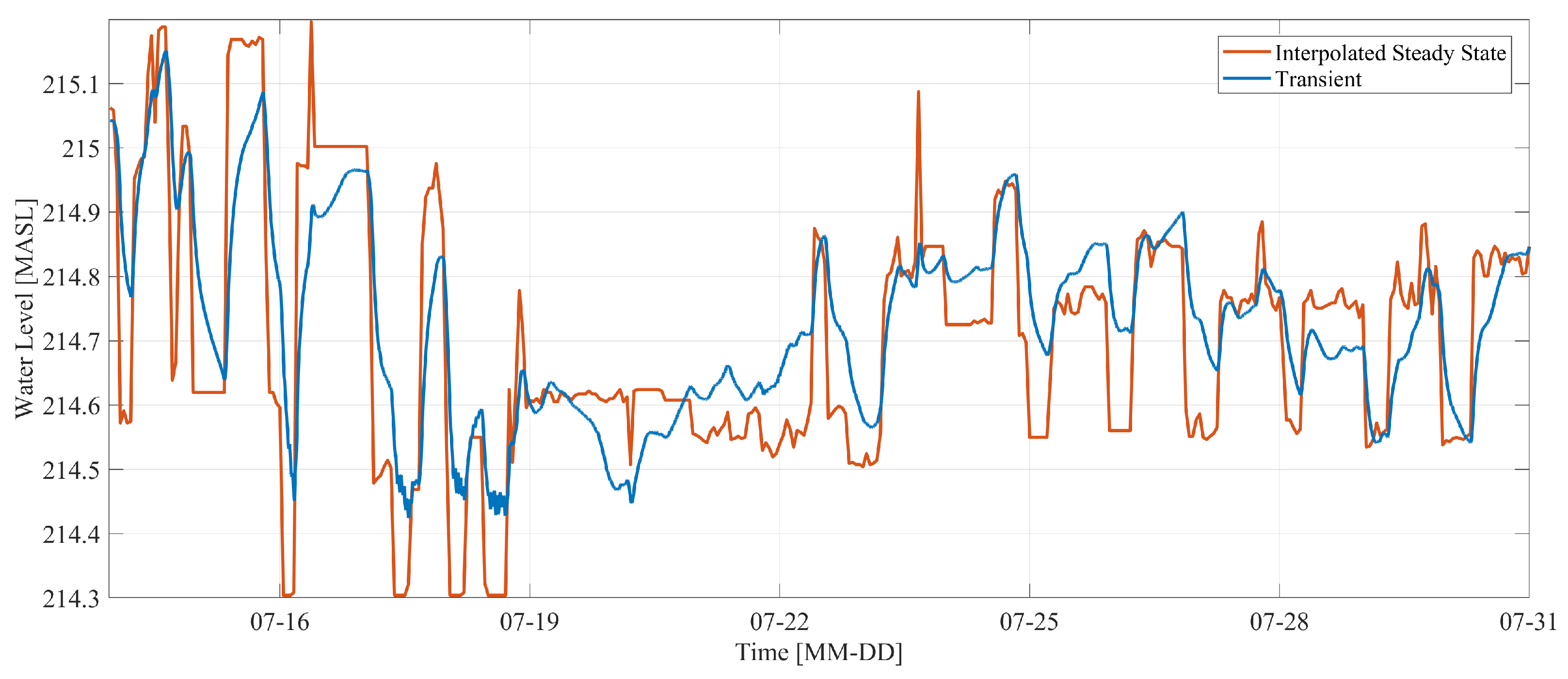
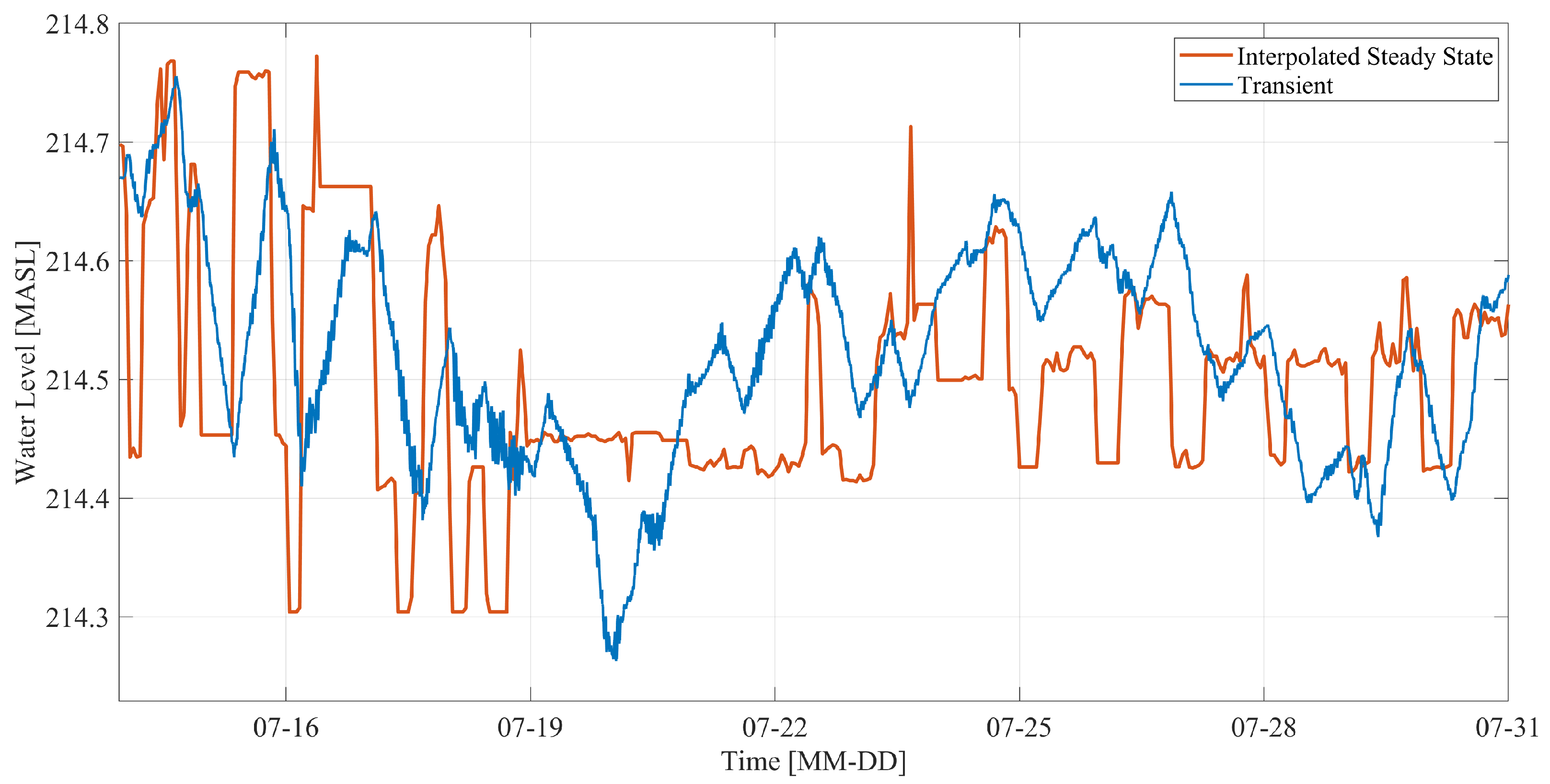
The steady-state cases were estimated manually by choosing different flow conditions, where the criterion was the up- and downstream discharge, and the WSE remained somewhat constant during 2 h. This was hard to find during the simulated period, which could introduce errors into the choice of simulated steady-state cases. Another approach of estimating the steady-state cases might be applied and lead to more accurate results. The choice of a steady-state or transient simulation is especially important when looking at the long-term effects on habitat. The steady-state cases were chosen for a time span during summer, but the downstream reservoir WSE varies depending on the time of the year. The steady-state flows should therefore be chosen over a wider time span to include the high variations during the season. Steady-state interpolation works well in rivers with stable, consistent flows. However, in rivers subjected to frequent hydropeaking or short-term regulation, it is not as accurate at predicting WSE either up- or downstream. Upstream, the steady-state follows the same patterns as the transient, but it over- and under-predicts the WSE with over ±0.1 m. Downstream, the damping properties of the river between different discharges are not taken into consideration where the response time is neglected because of the linear interpolation. However, a damping parameter based on the longitudinal length might be added to account for the neglect in damping [20].

The transient simulations are more time consuming to conduct but provide more accurate estimations of the hydraulic variables compared to steady-state interpolations. From the calibration, the maximum MAE was 0.087 m. Together with the MAE of 0.088 m and maximum absolute error of 0.4 m, the predicted WSE for the steady-state interpolation has a maximum error of up to 0.49 m, with a MAE of 0.175 m compared to the transient simulation. The advantage of a steady-state interpolated method is that the simulation times are shorter. This study employed a 2 h simulation time for 24 h in the model for the transient simulation, while the steady-state simulations only needed 1–3 h for stabilizing. Once the steady-state simulations were finished, the interpolation could be used to generate hydraulic results, which provide an advantage for longer time series. However, the simulation time for the transient case could be reduced further by using a larger time span for the output storage and using a larger time step by changing the Courant number while still ensuring stability. The hydraulic results are given to an output file during the required time span, so one does not need to wait for the whole simulation to finish to perform habitat studies but could couple these processes together. However, a transient simulation still presents challenges due to downstream boundary conditions. In cases where studies on environmental flows (E-flows) are required without performing field studies and experiments, the downstream boundary becomes a significant problem in low-sloping rivers between two hydropower plants. The water level boundary in the model had a significant impact on the downstream areas the river reached, roughly 4 km away from the boundary, which were affected by the set boundary. To solve the downstream boundary without going back to linear interpolation, a machine learning model might be developed. This model could be trained on data such as upstream and downstream discharge, reservoir water levels, and measured WSEs within the study region, and it might be able to predict the relationship and generate downstream boundary conditions for E-flows in these types of cases more accurately than interpolation alone.

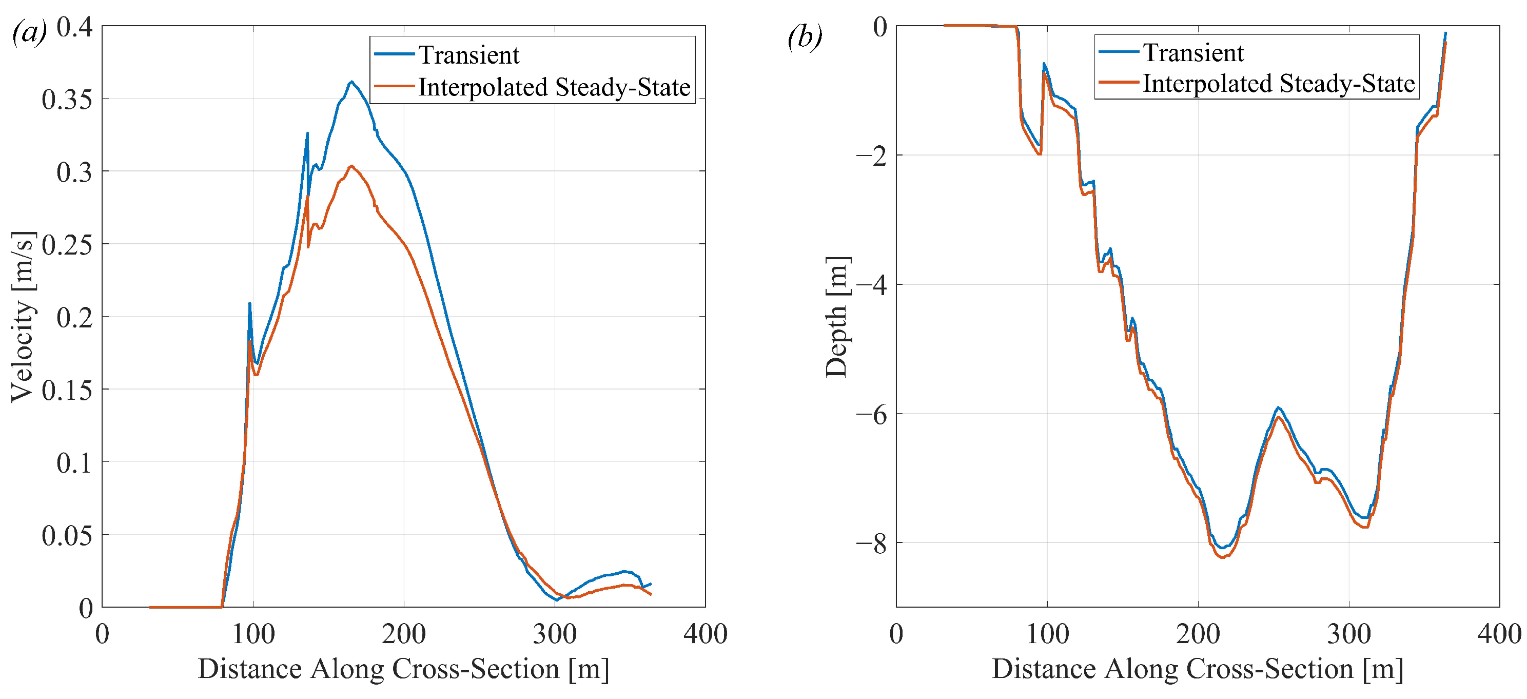
The suitable spawning area for European grayling differs between the methods over time, where the steady-state shows much more stable conditions compared to the transient state. The suitable spawning area is based on suitable depths and velocities. The velocity and depth differences between the methods in one cross section were 0.06 m/s and 0.15 m. Looking at the preferable range of depths and velocities, 0.3–0.5 m and 0.4–0.9 m/s [30] for European grayling, an error of 0.15 m and 0.06 m/s could make a significant difference on the suitable spawning grounds. 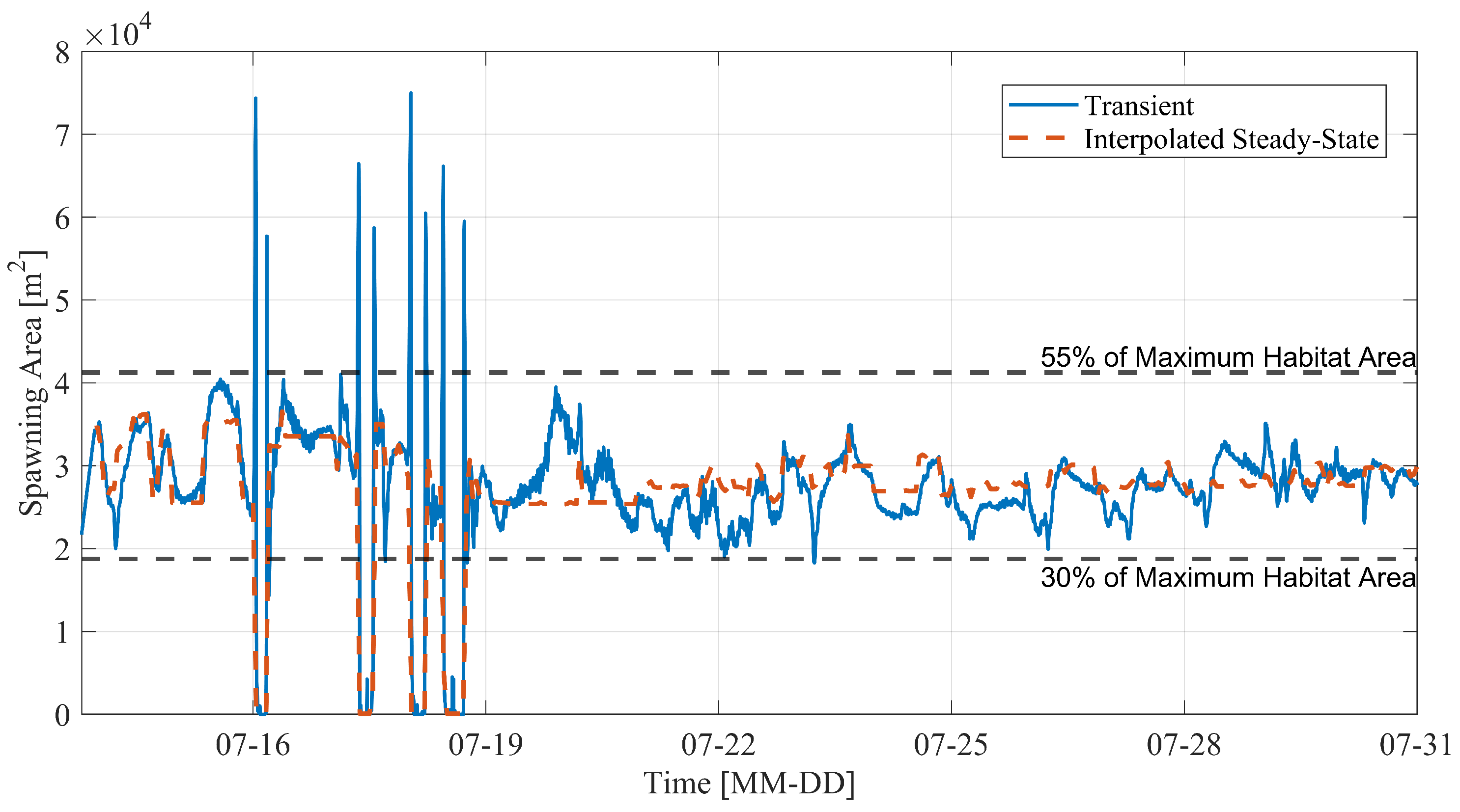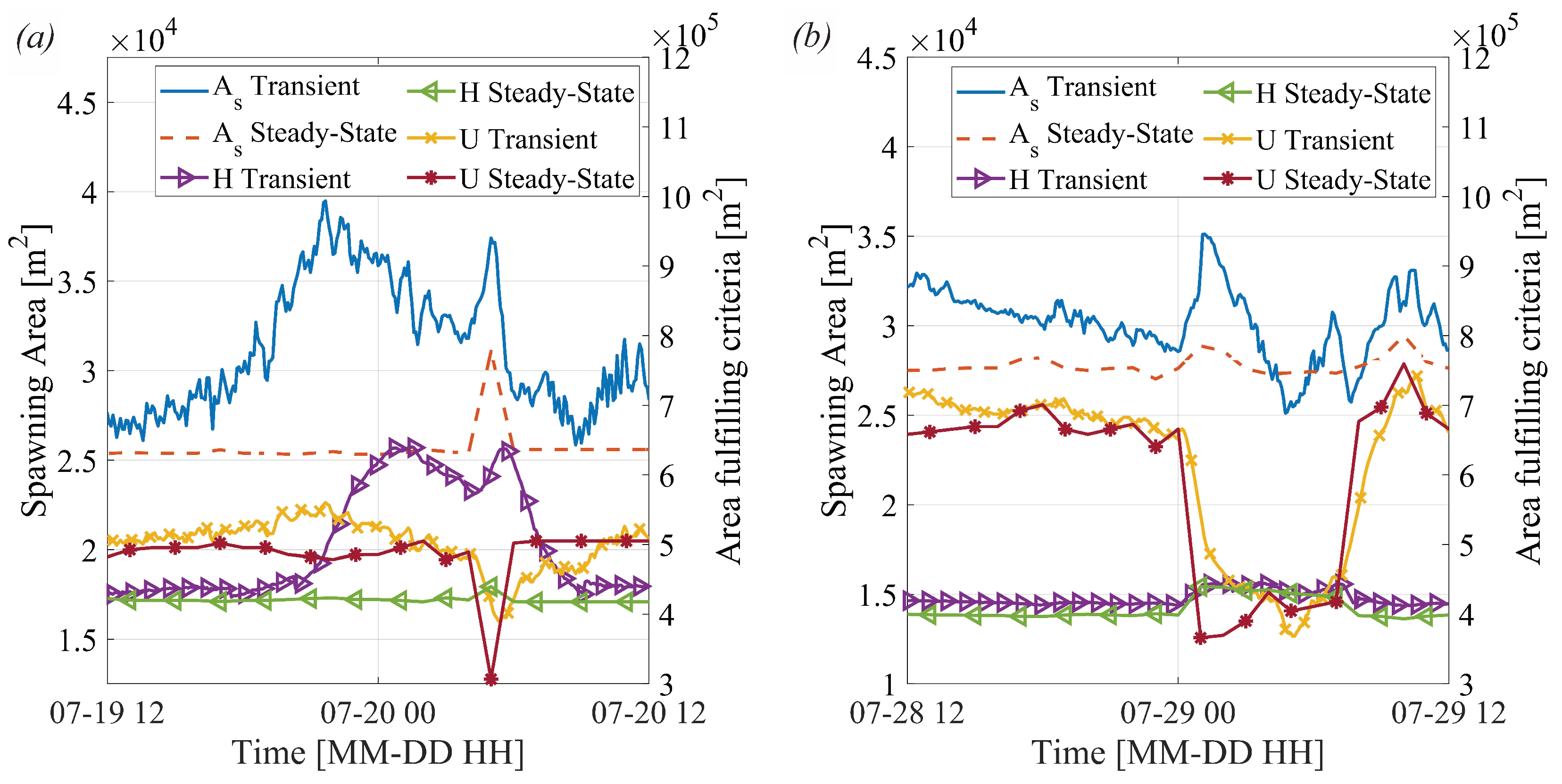The difference is especially seen around 19–21 July in Figure 11, where the suitable spawning ground for the transient simulation is higher than the steady-state interpolation. The comparison between steady-state interpolation and transient simulations reveals significant differences in Figure 12. In the first scenario, where the upstream discharge remains constant but downstream regulation affects water levels, depth variation accounts for the largest difference, with a 52.9% difference in available spawning depth and a 32.2% difference in total habitat area. This highlights the inability of steady-state interpolation to capture the downstream regulation. In the second scenario, an upstream down-ramping event causes a 38.8% overestimation of velocity-suitable habitat due to the steady-states immediate response to discharge changes. The transient model, which captures the gradual flow adjustments, provides a more accurate habitat estimation. The MAE in spawning habitat predictions for these cases is 5619 m² and 2614 m². For an IBM, this means a difference in available spawning habitat affecting the growth of redds and therefore also long-term growth in population. Temporal variability in habitat area influences fish behaviour, as fluctuations in spawning habitat impact both predation risk and survival rates, particularly for younger fish. A more dynamically varying habitat, which aligns with discharge fluctuations, may alter activity patterns, as habitat availability is often reduced at night and increases during the day. This pattern is evident in Figure 12b, where the transient simulation captures greater variation in spawning area compared to the steady-state interpolation. Since suitable spawning grounds shift over time, capturing the time-dependent habitat dynamics in hydropeaking rivers is crucial for accurately assessing how operational discharge schemes influence fish behaviour and survival.

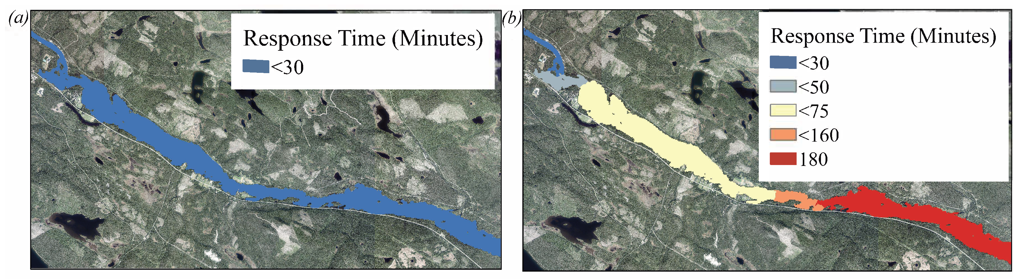
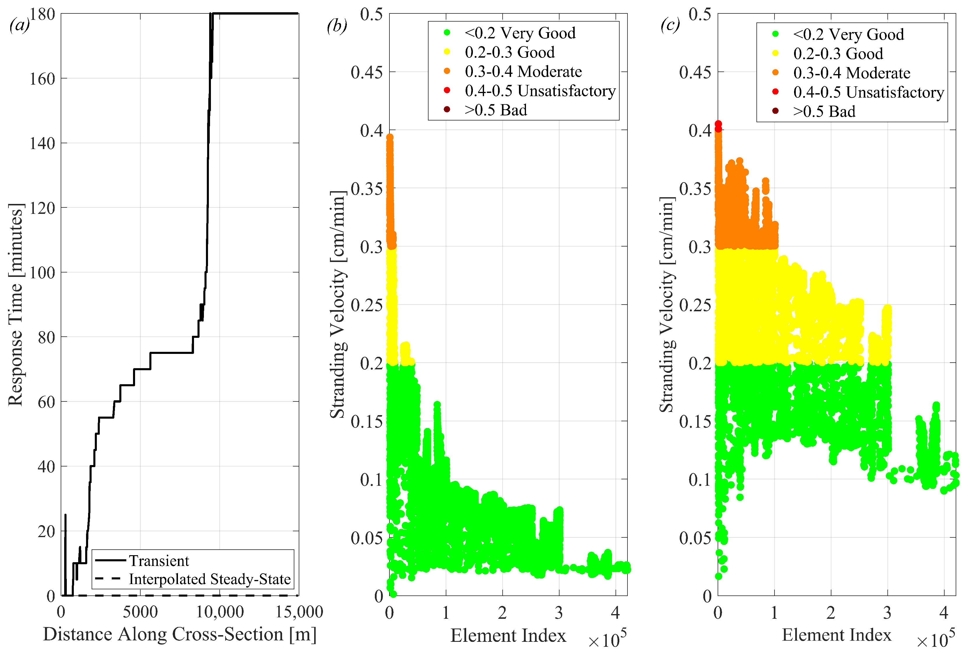
The WSE between the methods is differentiating over time. Upstream, the WSE is following a similar pattern as the transient simulation, but downstream, the damping is neglected. The response time is constant for the whole river for the steady-state interpolation so that the delayed response downstream is not captured by the model. A transient simulation will more accurately represent the damping and the different hydraulic stages across the river [6]. Capturing the hydraulic stages and the rivers longitudinal effects downstream [6] is important for evaluating the hydropeaking frequency effect on spawning habitat and stranding risks [10]. The stranding risks show large differences, where the steady-state shows a much higher risk in more elements than the transient simulation. As a result, the steady-state approach dewaters potential habitat cells much faster than the transient simulation. This results in fewer habitat cells for the fish to choose from in the IBM model, potentially causing redd dewatering and increased mortality, resulting in a negative impact on the fish population. Including the correct down-ramping rates as an output to compare with the thresholds could help with understanding where and when the fish perish and under which flow circumstances. The stranding risk was calculated for only one down-ramping event. In a low-sloping river with low-sloping banks, the lateral down-ramping rate [36] together with the seasonal variation of baseflow [35] and reservoir water level during the year could be more interesting to evaluate the stranding risk rather than one isolated down-ramping event.

The scouring risks of redds estimated from the possible sediment transport of suitable substrate are higher for the transient simulations upstream, where the steady-state underestimated the high peaks and overestimated the bed shear stress downstream. The steady-state interpolation method did, however, give a good estimation for lower flow. The possible areas with suitable spawning gravel are defined for each cell in the IBM either by confirming these in the field or using the bed shear stress. Confirming the substrate in situ would reduce the need of analysing the bed shear stress. However, for restoration measures that include adding substrate, the bed shear stress is important to evaluate in order to understand the risk of sediment being transported, eroded away, in the river. The peak bed shear stress is found in the beginning of the discharge increase, and it decreases while the flow remains constant. In previous studies, it was found that the peaks in bed shear stress are not always proportional to the discharge, meaning that the transition periods between base and peak flows are more important to study rather than the peak flow as an isolated case [43]. The findings of the study [43] recommended that investigations of restoration measures should consider the unsteady transition period and nonlinear behaviour to understand the impact that flow alterations with high unsteadiness, such as hydropeaking, could have on the rivers’ topography. The transient simulation in this study shows that initial high peaks of bed shear stress when changing the flow regime could not be captured by the steady-state interpolation method. Future restoration measures by adding suitable substrate sizes in spawning areas should consider the transient bed shear stress to ensure the stability of the bed and added substrate during different flow regimes over time.

In future work, a sensitivity analysis regarding the hydraulic inputs to IBMs can be considered to see how different hydraulic conditions can affect fish population dynamics in the long-term. The analysis in this study did not consider the additional complexity and uncertainty that arise when including more variables such as temperature and fish behaviour during different flow conditions and times of the day. The risk of sediment transport in this study is a simplified case and could be developed further by analysing the bed-load transport with a representative transport formula in Delft3D FM D-Morphology to analyse the time-dependent impacts of hydropeaking and include the additional complexity of a riverbed. This could further help to understand the dynamic relationship between hydropeaking rivers, seasonal flows, and the effect on the fish life-cycle and habitat enhancement.

6. Conclusions

This study highlights the challenges of applying hydraulic models for habitat assessments in a high-frequency hydropeaking river where both up- and downstream regulations influence the water levels. The selection between steady-state interpolation and transient simulation for habitat studies must be made with an understanding of how the hydraulic variables are affected by both up- and downstream dynamics and if there is ever a steady-state condition in the river. The hydraulic output from steady-state models should be validated against transient simulations to assess their ability to capture flow variations over time. While steady-state interpolation can provide a preliminary estimation, it introduces additional errors into habitat studies that are already based on generalised data from the literature. This approach neglects the damping within the river, affecting both the spawning areas over time and the dewatering rates. Moreover, it fails to capture the high peaks in bed shear stress, which are important for assessing spawning ground suitability and the scouring risk of redds.

The primary challenge of transient simulations lies in their long computation times, particularly when using fine mesh resolutions. Long-term habitat studies (spanning 3–5 years) that incorporate hourly hydropeaking fluctuations and daily variations would require extensive simulation run times and large storage capacities for model outputs. Additionally, downstream boundary conditions pose a challenge in this system, as water levels are influenced by downstream regulation. In this study, measured water levels were used as the downstream boundary. However, for E-flow assessments, interpolating the downstream boundary is not feasible when regulation effects are significant.

In rivers with stable flow conditions, steady-state interpolation can serve as a useful tool to reduce simulation time and evaluate new operational flow strategies for habitat improvement. In this study, the steady-state interpolation approach resulted in a MAE of 2910 m² in estimating spawning habitat area. Although this time period had relatively stable conditions considering the annual variation in reservoir water levels, steady-state interpolation seems unsuitable for this river during any time of the year.

In more dynamic rivers, and for decision making regarding river management from a long-term perspective for fish habitat restoration, a steady-state interpolation approach may be unsuitable, and a transient time dependent solution is preferable.