
Discrete Element Method Simulation of Loess Tunnel Erosion


Abstract
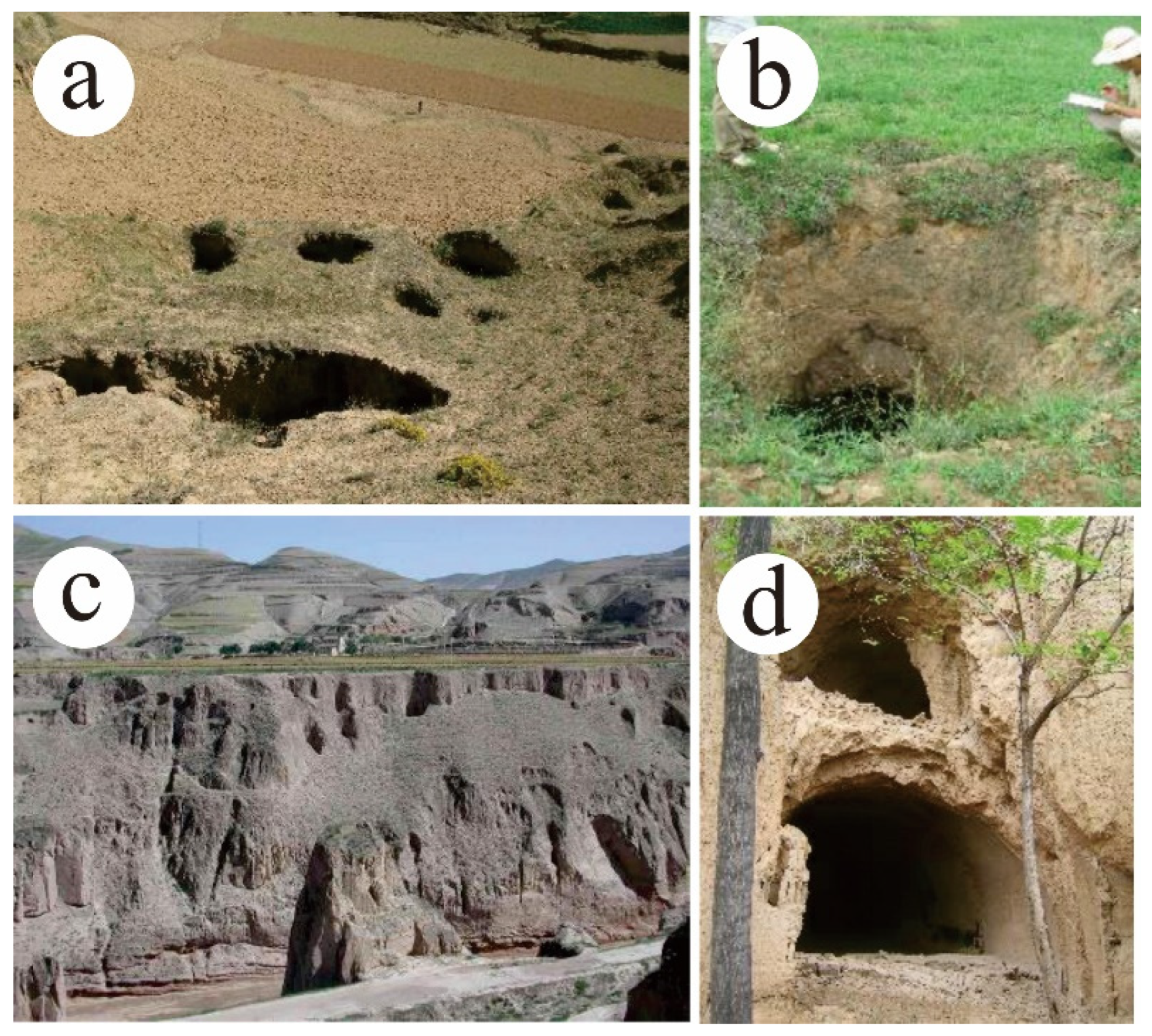
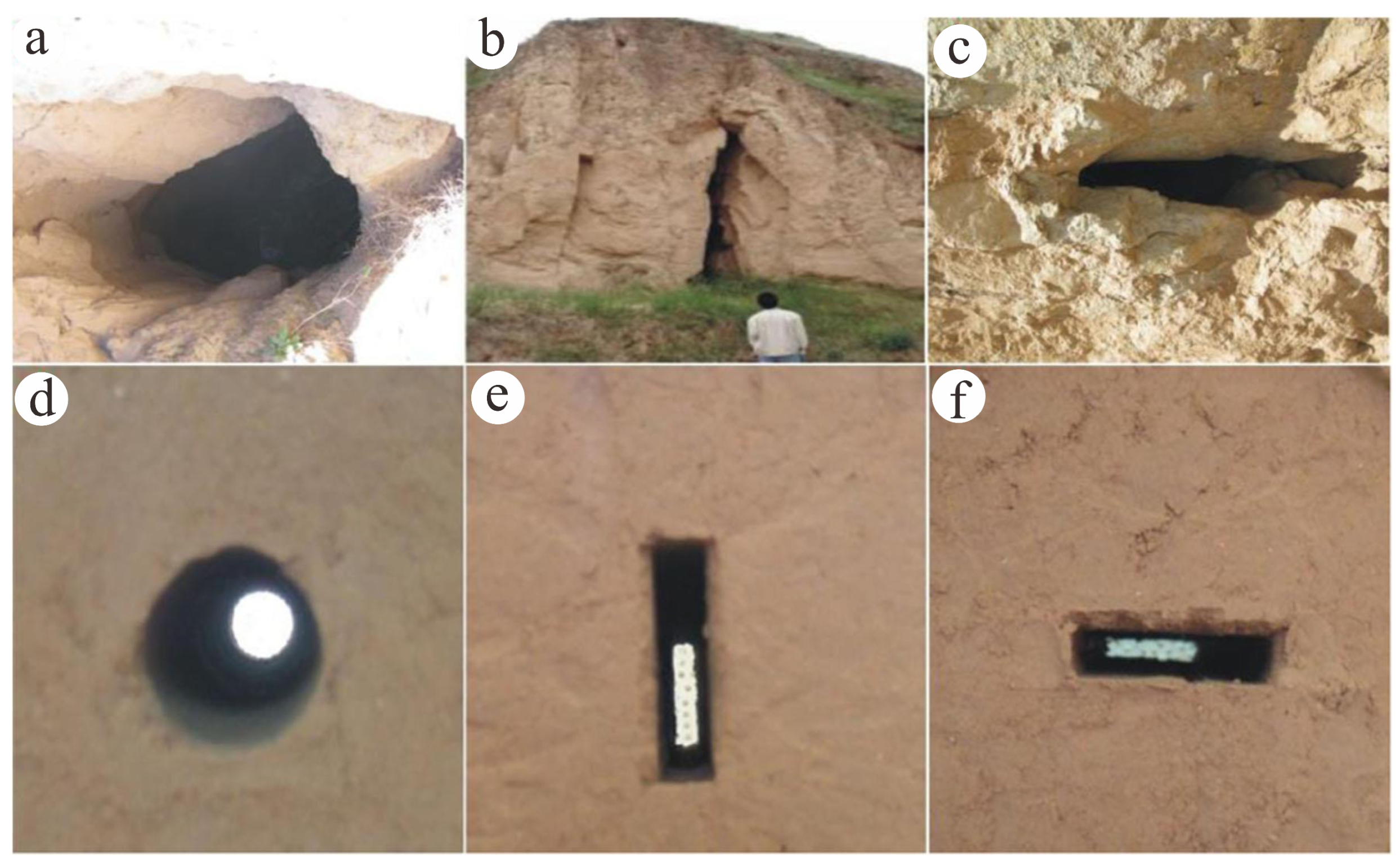
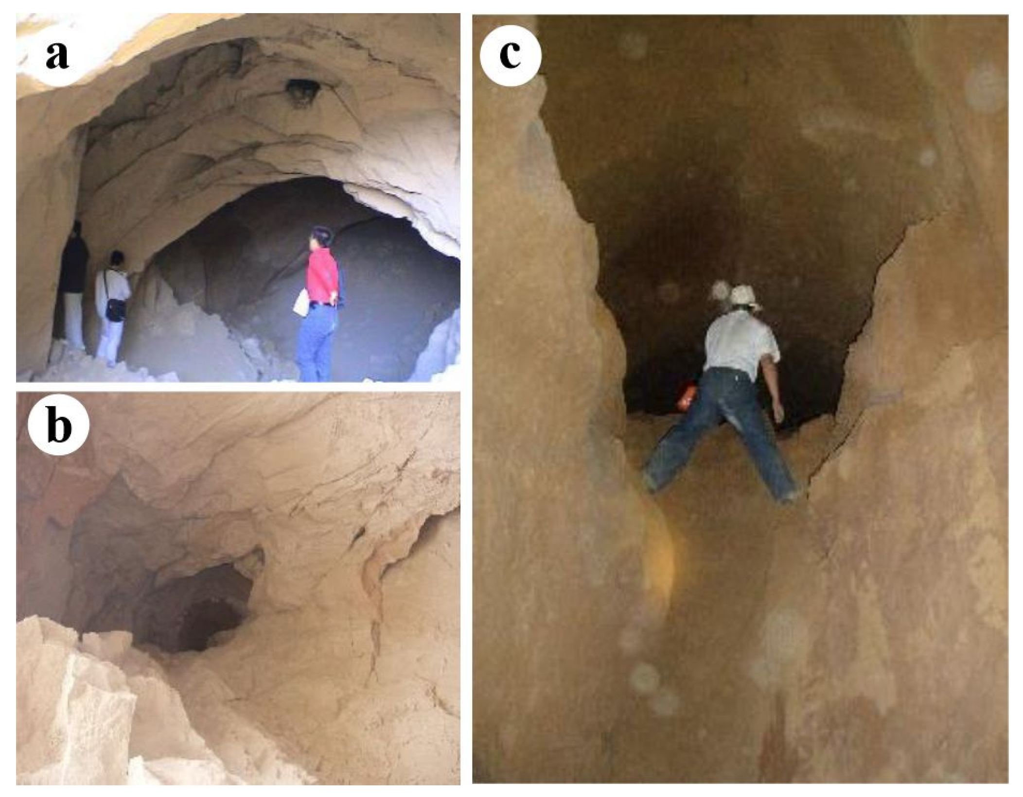
1. Introduction
2. Materials and Methods
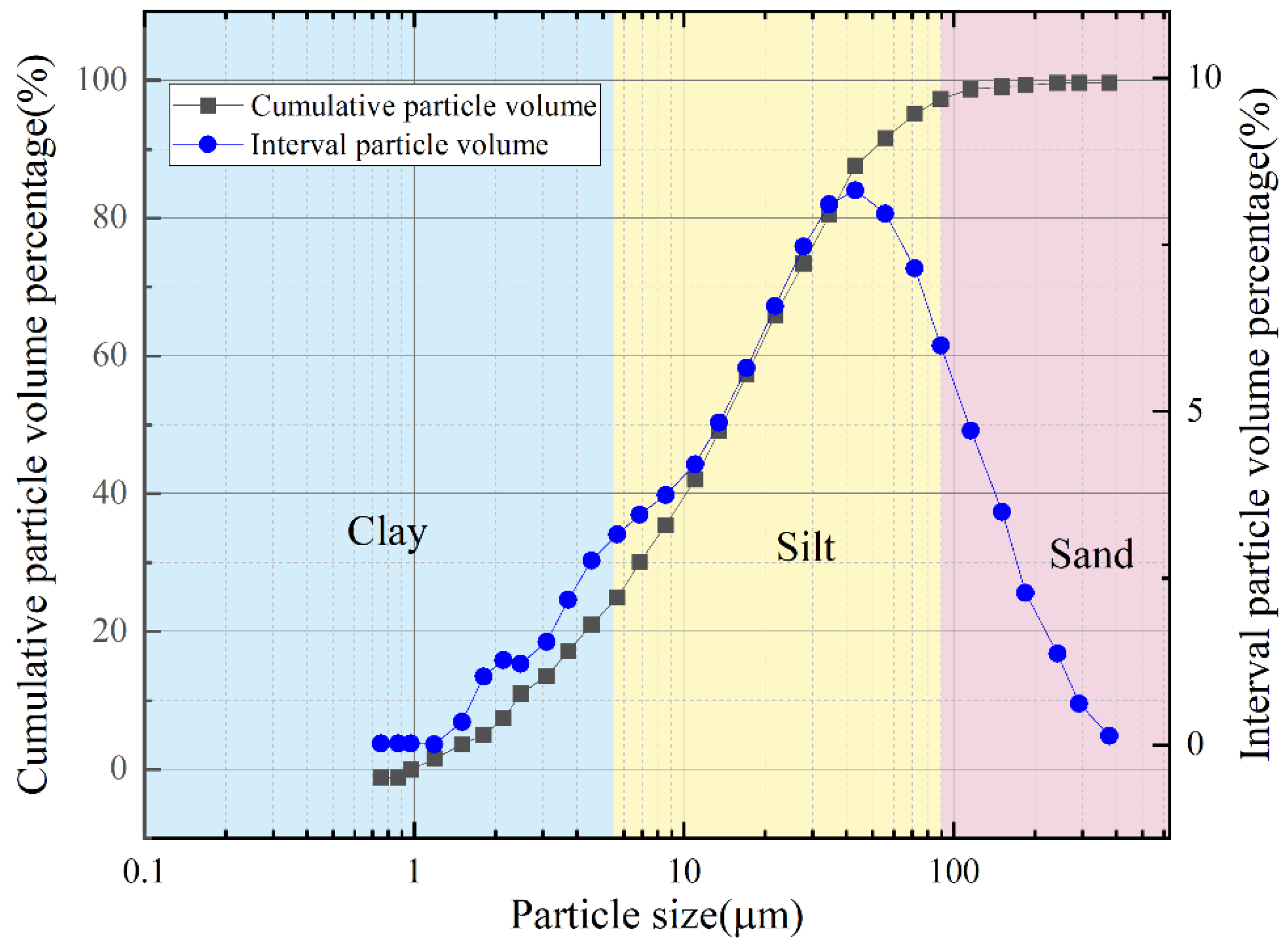
2.1. Materials
2.2. Overview of Discrete Element Method
2.3. Model Establishment
2.4. Calibration of the Model
2.4.1. Calibration of Contact Parameters
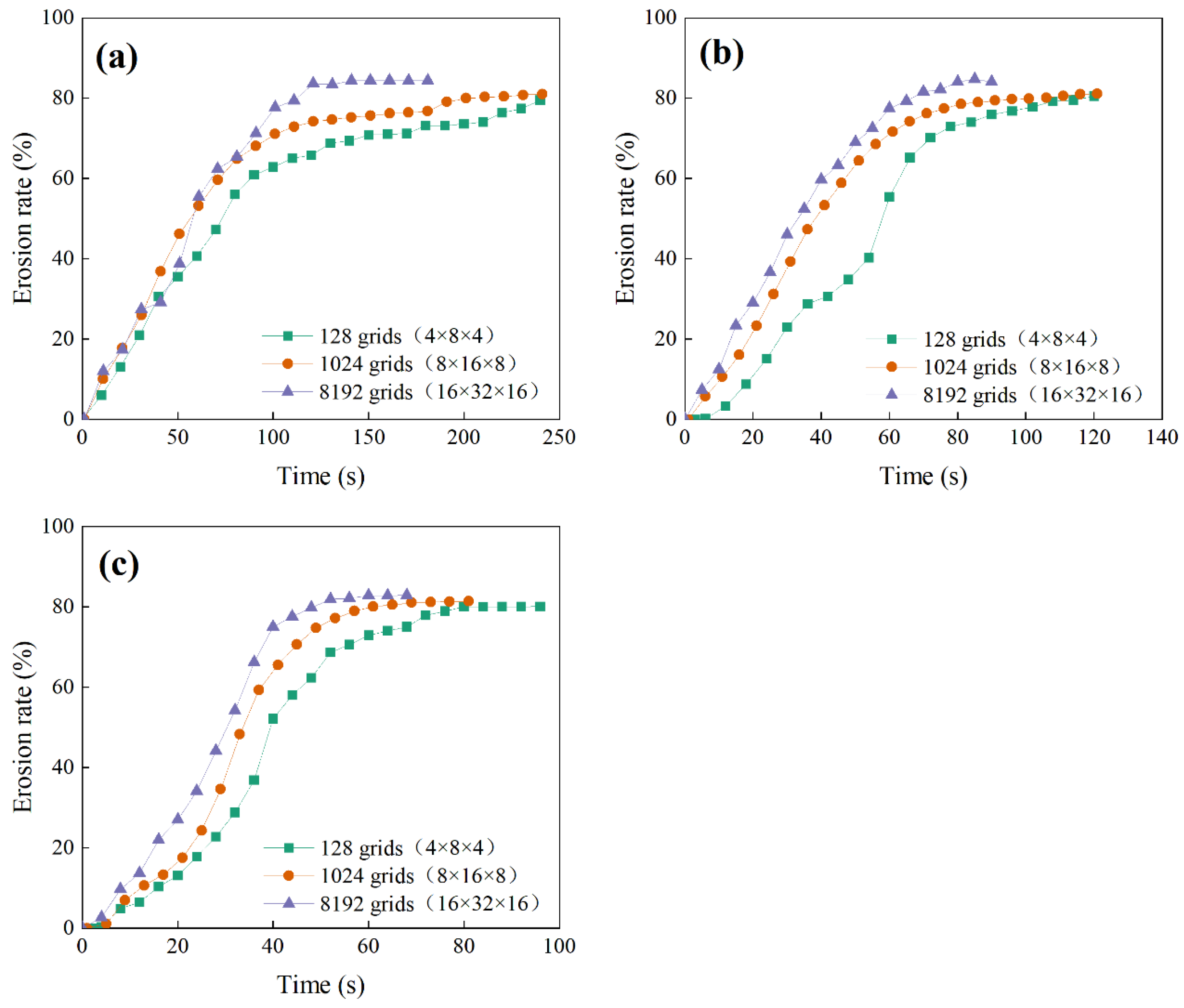
2.4.2. Adjustment of the Number of Fluid Grids
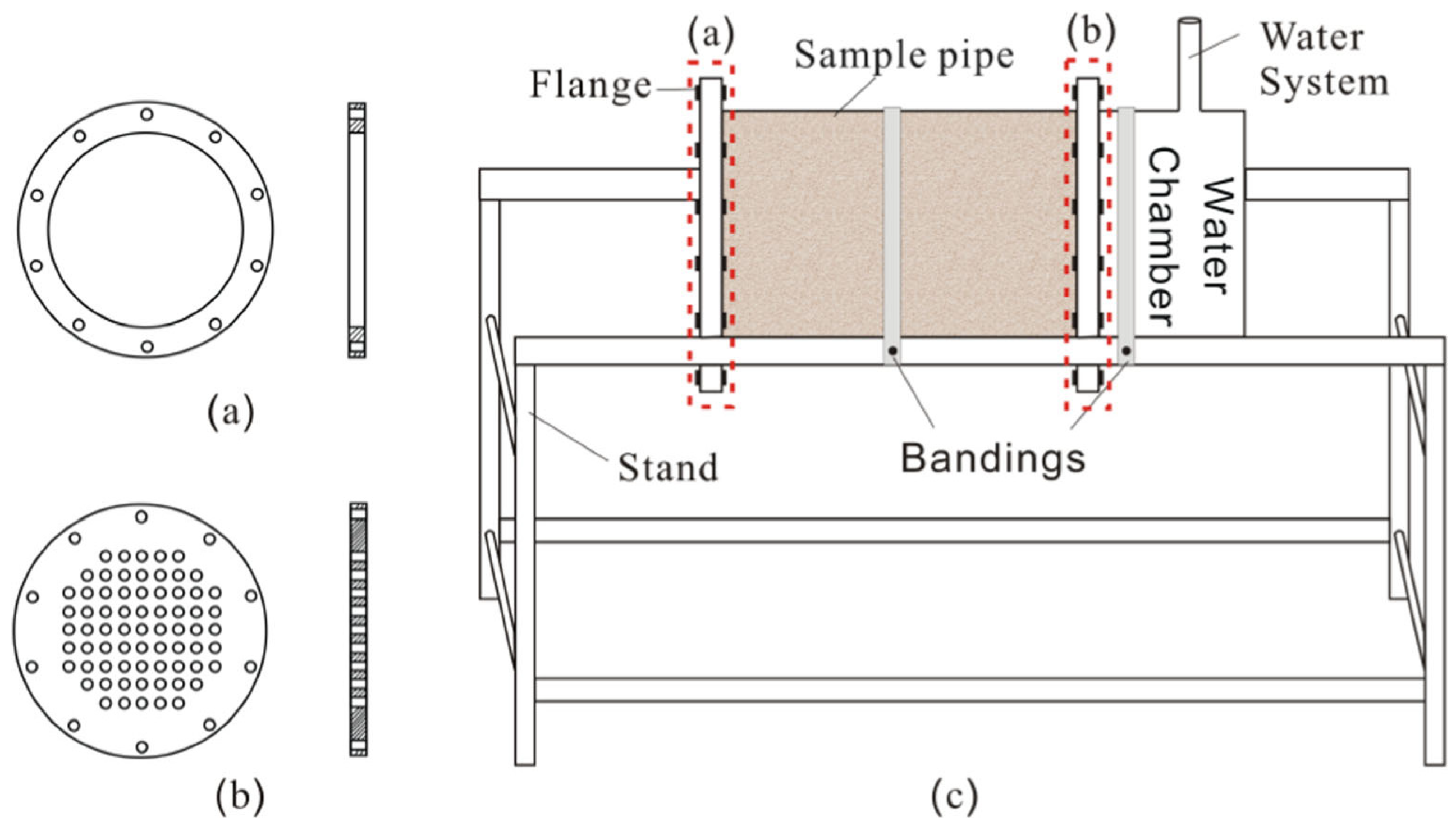
2.4.3. Comparison and Verification with Physical Experiments
3. Results and Discussion
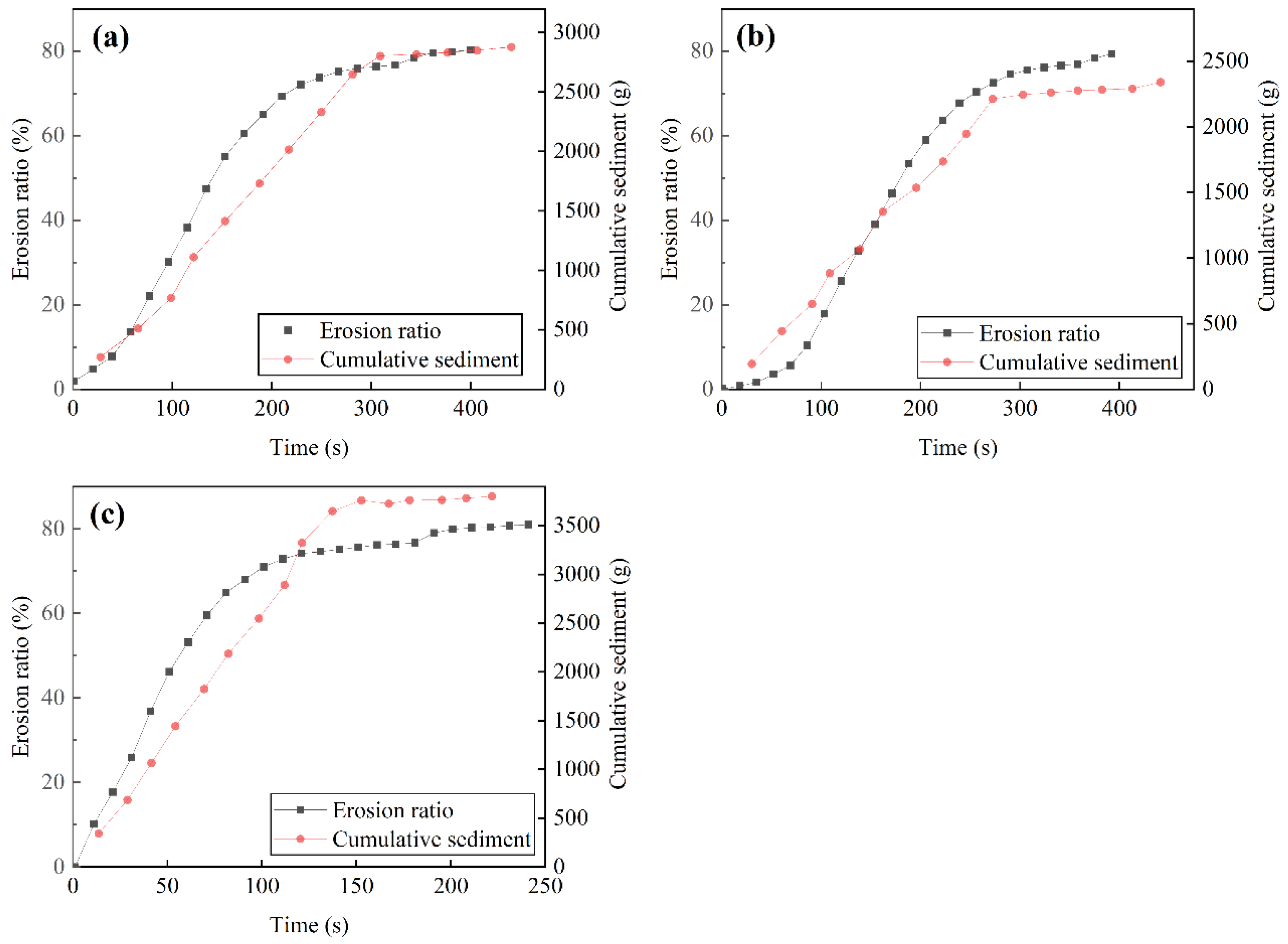
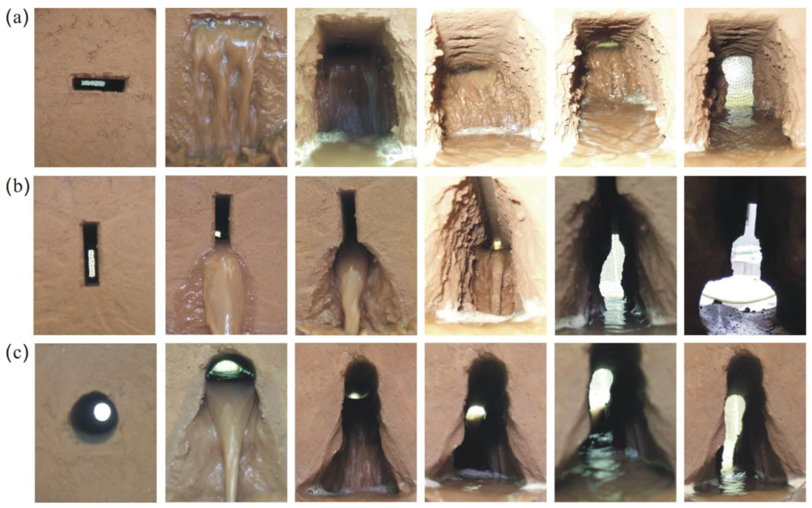
3.1. Erosion Process
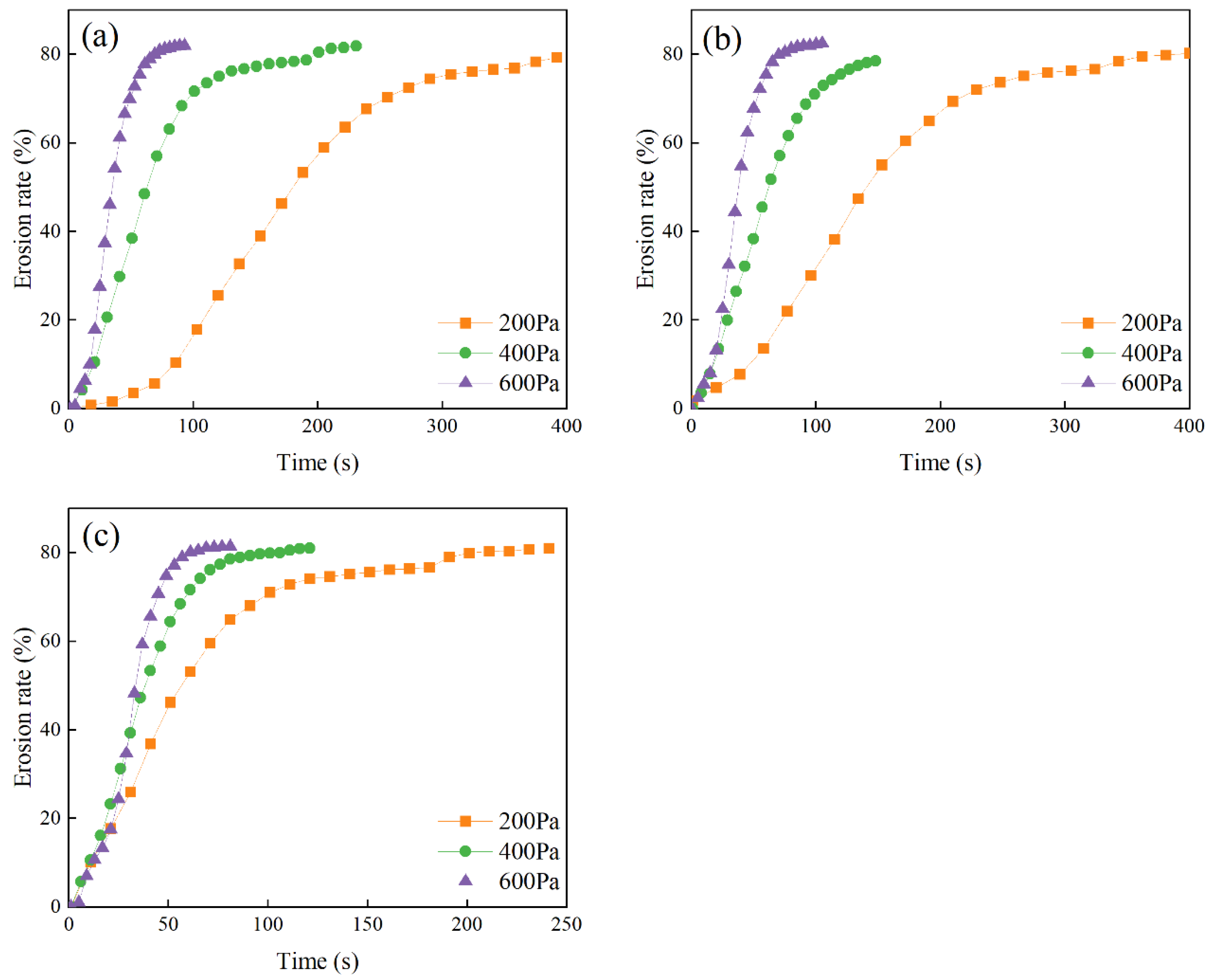
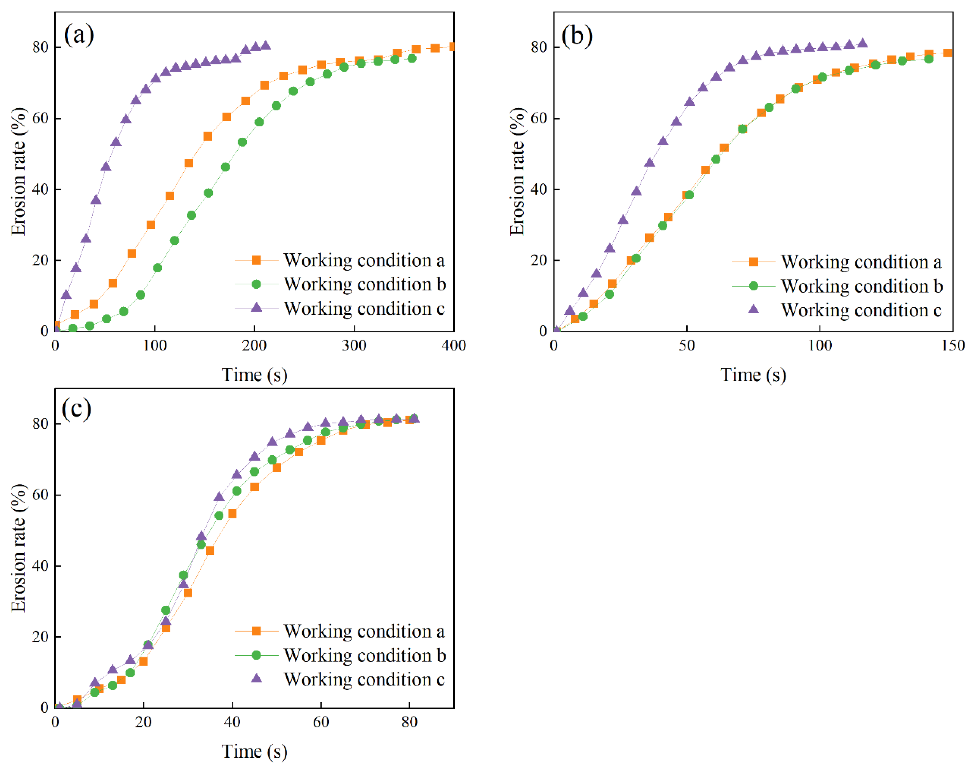
3.2. Erosion Rate
3.3. Discussion
4. Conclusions
Author Contributions
Funding
Data Availability Statement
Acknowledgments
Conflicts of Interest
References
- Liu, Y.; Fu, B.; Lü, Y.; Wang, Z.; Gao, G. Hydrological responses and soil erosion potential of abandoned cropland in the Loess Plateau China. Geomorphology 2012, 138, 404–414. [Google Scholar] [CrossRef]
- Tsunekawa, A.; Liu, G.; Yamanaka, N.; Du, S. Restoration and Development of the Degraded Loess Plateau, China; Springer: Tokyo, Japan, 2014. [Google Scholar] [CrossRef]
- Li, P.; Mu, X.; Holden, J.; Wu, Y.; Irvine, B.; Wang, F.; Gao, P.; Zhao, G.; Sun, W. Comparison of soil erosion models used to study the Chinese Loess Plateau. Earth Sci. Rev. 2017, 170, 17–30. [Google Scholar] [CrossRef]
- Wu, B.; Wang, Z.; Zhang, Q.; Shen, N. Distinguishing transport-limited and detachment-limited processes of interrill erosion on steep slopes in the Chinese loessial region. Soil Tillage Res. 2018, 177, 88–96. [Google Scholar] [CrossRef]
- Valentin, C.; Poesen, J.; Li, Y. Gully erosion: Impacts, factors and control. CATENA 2005, 63, 132–153. [Google Scholar] [CrossRef]
- Pimentel, D. Soil erosion: A food and environmental threat. Environ. Dev. Sustain. 2006, 8, 119–137. [Google Scholar] [CrossRef]
- Wang, L.; Shao, M.A.; Wang, Q.; Gale, W.J. Historical changes in the environment of the Chinese Loess Plateau. Environ. Sci. Pol. 2006, 9, 675–684. [Google Scholar] [CrossRef]
- Bouchnak, H.; Felfoul, M.S.; Boussema, M.R.; Snane, M.H. Slope and rainfall effects on the volume of sediment yield by gully erosion in the souar lithologic formation (tunisia). CATENA 2009, 78, 170–177. [Google Scholar] [CrossRef]
- Li, X.A.; Wang, L.; Hong, B.; Li, L.C.; Liu, J.; Lei, H. Erosion characteristics of loess tunnels on the Loess Plateau: A field investigation and experimental study. Earth Surf. Proc. Land. 2020, 45, 1945–1958. [Google Scholar] [CrossRef]
- Tao, H.; Tao, J. Quantitative analysis of piping erosion micro-mechanisms with coupled CFD and DEM method. Acta Geotech. 2017, 12, 573–592. [Google Scholar] [CrossRef]
- Verachtert, E.; Van Den Eeckhaut, M.; Martínez-Murillo, J.F.; Nadal-Romero, E.; Poesen, J.; Devoldere, S.; Wijnants, N.; Deckers, J. Impact of soil characteristics and land use on pipe erosion in a temperate humid climate: Field studies in Belgium. Geomorphology 2013, 192, 1–14. [Google Scholar] [CrossRef]
- Chaplot, V. Impact of terrain attributes, parent material and soil types on gully erosion. Geomorphology 2013, 186, 1–11. [Google Scholar] [CrossRef]
- Verachtert, E.; Van Den Eeckhaut, M.; Poesen, J.; Deckers, J. Factors controlling the spatial distribution of soil piping erosion on loess-derived soils: A case study from central Belgium. Geomorphology 2010, 118, 339–348. [Google Scholar] [CrossRef]
- Hosseinalizadeh, M.; Kariminejad, N.; Rahmati, O.; Keesstra, S.; Alinejad, M.; Behbahani, A.M. How can statistical and artificial intelligence approaches predict piping erosion susceptibility? Sci. Total Environ. 2019, 646, 1554–1566. [Google Scholar] [CrossRef] [PubMed]
- Li, Z.; Zhang, Y.; Zhu, Q.; Yang, S.; Li, H.; Ma, H. A gully erosion assessment model for the Chinese Loess Plateau based on changes in gully length and area. CATENA 2017, 148, 195–203. [Google Scholar] [CrossRef]
- Zheng, F.; He, X.; Gao, X.; Zhang, C.; Tang, K. Effects of erosion patterns on nutrient loss following deforestation on the Loess Plateau of China. Agric. Ecosyst. Environ. 2005, 108, 85–97. [Google Scholar] [CrossRef]
- Zhu, T.X. Tunnel development over a 12 year period in a semi-arid catchment of the Loess Plateau, China. Earth Surf. Proc. Land. 2003, 28, 507–525. [Google Scholar] [CrossRef]
- Zhu, T.X. Gully and tunnel erosion in the hilly Loess Plateau region, China. Geomorphology 2012, 153–154, 144–155. [Google Scholar] [CrossRef]
- Wang, L.; Li, X.A.; Zheng, Z.Y.; Zheng, H.; Ren, Y.; Chen, W.; Lei, H. Analysis of the slope failure mechanism a under tunnel erosion environment in the south-eastern Loess Plateau in China. CATENA 2022, 212, 106039. [Google Scholar] [CrossRef]
- Fannin, R.J.; Slangen, P. On the distinct phenomena of suffusion and suffosion. Géotech. Lett. 2014, 4, 289–294. [Google Scholar] [CrossRef]
- Nguyen, C.D.; Benahmed, N.; Andò, E.; Sibille, L.; Philippe, P. Experimental investigation of microstructural changes in soils eroded by suffusion using X-ray tomography. Acta Geotech. 2019, 14, 749–765. [Google Scholar] [CrossRef]
- Chen, T.; Hu, Z.; Yang, Z.; Zhang, Y. A resolved CFD–DEM investigation into the onset of suffusion: Effect of confining pressure and stress anisotropy. Int. J. Numer. Anal. Methods Geomech. 2023, 47, 3018–3043. [Google Scholar] [CrossRef]
- Wang, X.; Huang, B.; Tang, Y.; Hu, T.; Ling, D. Microscopic mechanism and analytical modeling of seepage-induced erosion in bimodal soils. Comput. Geotech. 2022, 141, 104527. [Google Scholar] [CrossRef]
- Zhang, Y.; Zhao, M.; Kwok, K.C.S.; Liu, M.M. Computational fluid dynamics–discrete element method analysis of the onset of scour around subsea pipelines. Appl. Math. Model. 2015, 39, 7611–7619. [Google Scholar] [CrossRef]
- Wang, L.; Li, X.A.; Li, L.C.; Hong, B.; Liu, J. Experimental study on the physical modeling of loess tunnel-erosion rate. Bull. Eng. Geol. Environ. 2019, 78, 5827–5840. [Google Scholar] [CrossRef]
- Zhao, J.; Shan, T. Coupled CFD–DEM simulation of fluid–particle interaction in geomechanics. Powder Technol. 2013, 239, 248–258. [Google Scholar] [CrossRef]
- Sibille, L.; Lominé, F.; Poullain, P.; Sail, Y.; Marot, D. Internal erosion in granular media: Direct numerical simulations and energy interpretation. Hydrol. Process. 2015, 29, 2149–2163. [Google Scholar] [CrossRef]
- Sun, J.; Li, X.-A.; Li, J.; Zhang, J.; Zhang, Y. Numerical investigation of characteristics and mechanism of tunnel erosion of loess with coupled CFD and DEM method. CATENA 2023, 222, 106729. [Google Scholar] [CrossRef]
- Wen, F.; Li, X.A.; Yang, W.; Li, J.; Zhou, B.; Gao, R.; Lei, J.W. Mechanism of loess planar erosion and numerical simulation based on CFD-DEM coupling model. Environ. Earth Sci. 2023, 82, 197. [Google Scholar] [CrossRef]


| Natural Density (g/cm3) | Natural Water Content (%) | Clay (mm), <0.005 | Silt (mm), 0.075~0.0005 | Sand (mm), 2~0.075 |
|---|---|---|---|---|
| 1.53 | 7.5 | 15.6 | 70.5 | 13.9 |
| Computation Model | Parameter | Numerical Value |
|---|---|---|
| Solid State Systems (DEM) | Particle density (kg/m3) | 1500 |
| Bond modulus (kPa) | 4.0 × 10⁶ | |
| Effective modulus, Ec (Pa) | 1.0 × 10⁷ | |
| porosity | 0.35 | |
| Stiffness ratio (kn/ks) | 1.5 | |
| Coefficient of friction | 0.3 | |
| Fluid Dynamics (CFD) | Density (kg/m3) | 1.0 × 10³ |
| Fluid viscosity coefficient (Pa·s) | 1.0 × 10⁻³ |
Disclaimer/Publisher’s Note: The statements, opinions and data contained in all publications are solely those of the individual author(s) and contributor(s) and not of MDPI and/or the editor(s). MDPI and/or the editor(s) disclaim responsibility for any injury to people or property resulting from any ideas, methods, instructions or products referred to in the content. |
© 2025 by the authors. Licensee MDPI, Basel, Switzerland. This article is an open access article distributed under the terms and conditions of the Creative Commons Attribution (CC BY) license (https://creativecommons.org/licenses/by/4.0/).
Share and Cite
Dong, H.; Li, X.; Wang, W.; An, M. Discrete Element Method Simulation of Loess Tunnel Erosion. Water 2025, 17, 1020. https://doi.org/10.3390/w17071020
Dong H, Li X, Wang W, An M. Discrete Element Method Simulation of Loess Tunnel Erosion. Water. 2025; 17(7):1020. https://doi.org/10.3390/w17071020
Chicago/Turabian StyleDong, Haoyang, Xian Li, Weiping Wang, and Mingzhu An. 2025. "Discrete Element Method Simulation of Loess Tunnel Erosion" Water 17, no. 7: 1020. https://doi.org/10.3390/w17071020
APA StyleDong, H., Li, X., Wang, W., & An, M. (2025). Discrete Element Method Simulation of Loess Tunnel Erosion. Water, 17(7), 1020. https://doi.org/10.3390/w17071020