
Optimal Scheduling Study of Hydro–Solar Complementary System Based on Improved Beluga Whale Algorithm


Abstract
1. Introduction
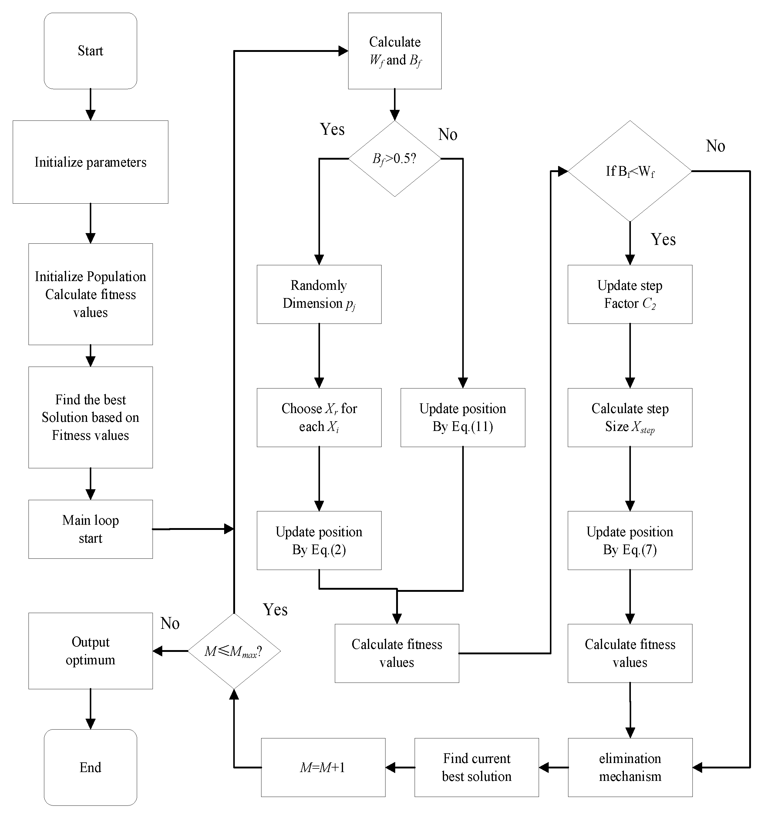
2. The Proposed Method
2.1. Beluga Whale Optimization (BWO)
2.1.1. Exploration Phase
2.1.2. Exploitation Phase
2.1.3. Whale Fall
2.2. Proposed Method
2.2.1. Spiral Motion
2.2.2. Elimination Mechanism
2.3. Framework of IBWO
2.4. Computational Complexity
3. Numerical Experiments to Verify the Performance of the IBWO Method
3.1. Benchmark Functions Set I
3.1.1. Classic Test Functions
3.1.2. Parameter Settings
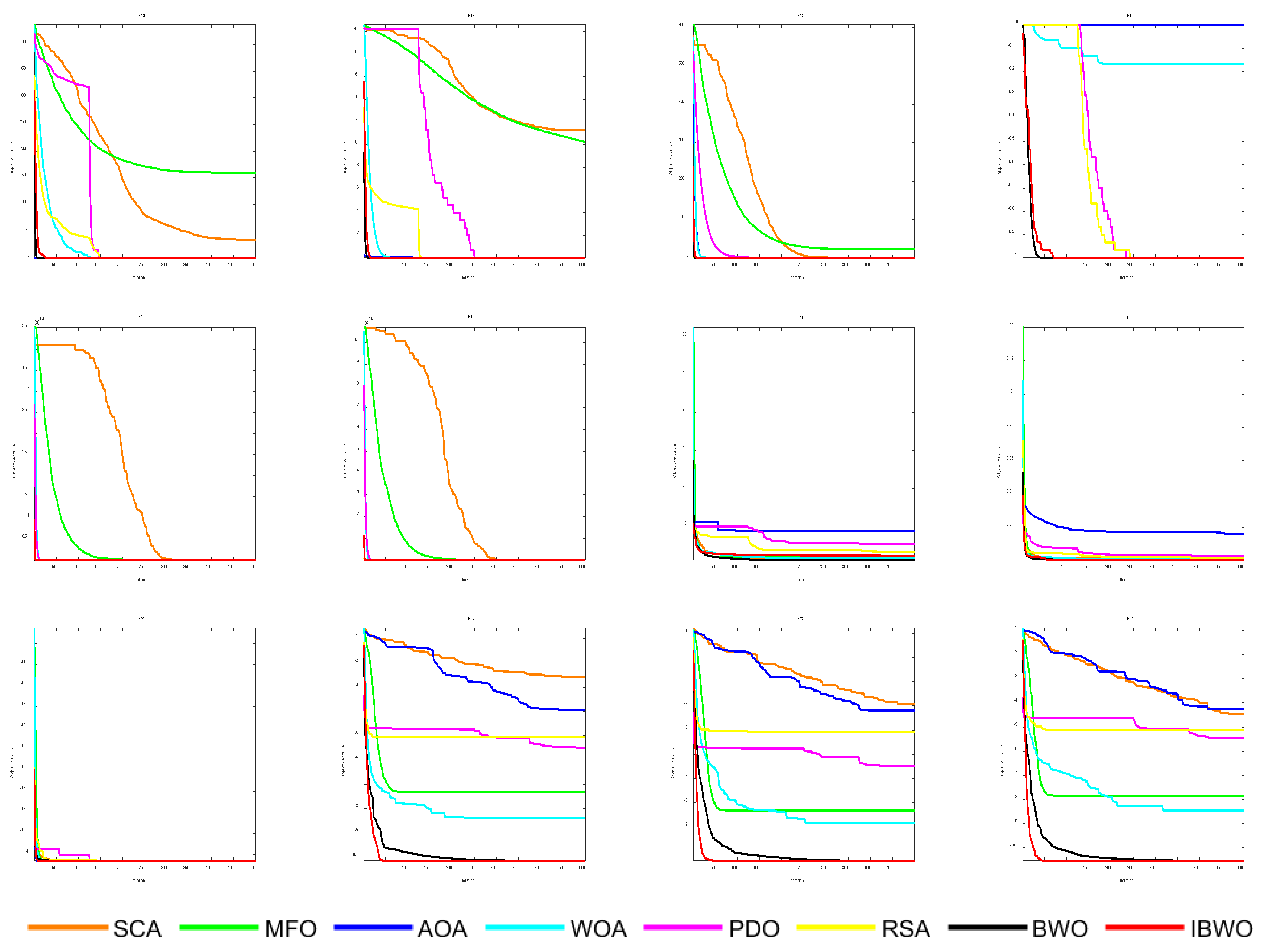
3.1.3. Experimental Results
3.2. Benchmark Functions Set II: IEEE CEC2017
3.2.1. CEC2017 Test Functions
3.2.2. Statistical Results Analysis
4. IBWO Algorithm for Solving the Optimal Scheduling Problem of Hydro–Solar Complementary System
4.1. Mathematical Model
4.1.1. Objective Function
4.1.2. Physical Constraints
4.2. Details of IBWO for the Optimal Scheduling Problem of Hydro–Solar Systems
4.2.1. Individual Structure and Swarm Initialization
4.2.2. Constraint Handling Method
- Constrained corridor
- 2.
- Constrained objective method
4.3. Overall Implementation Framework
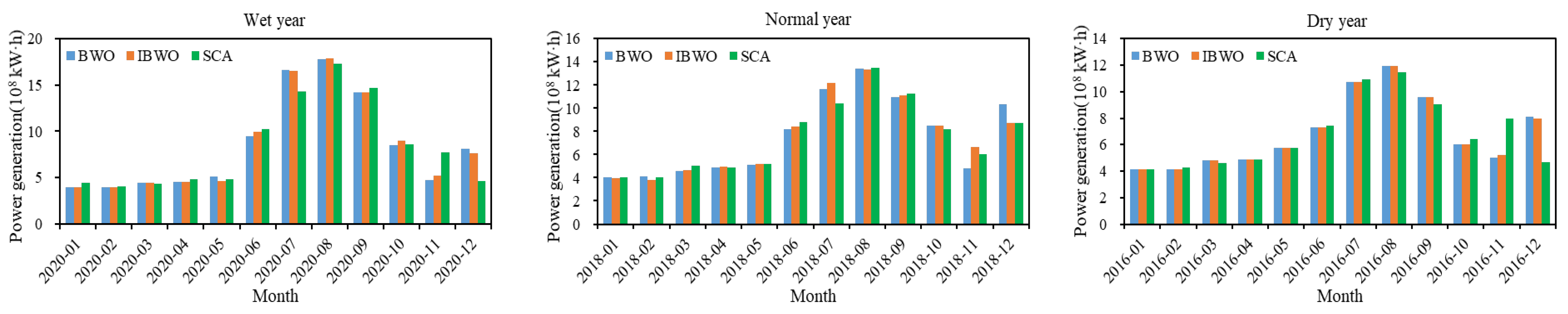
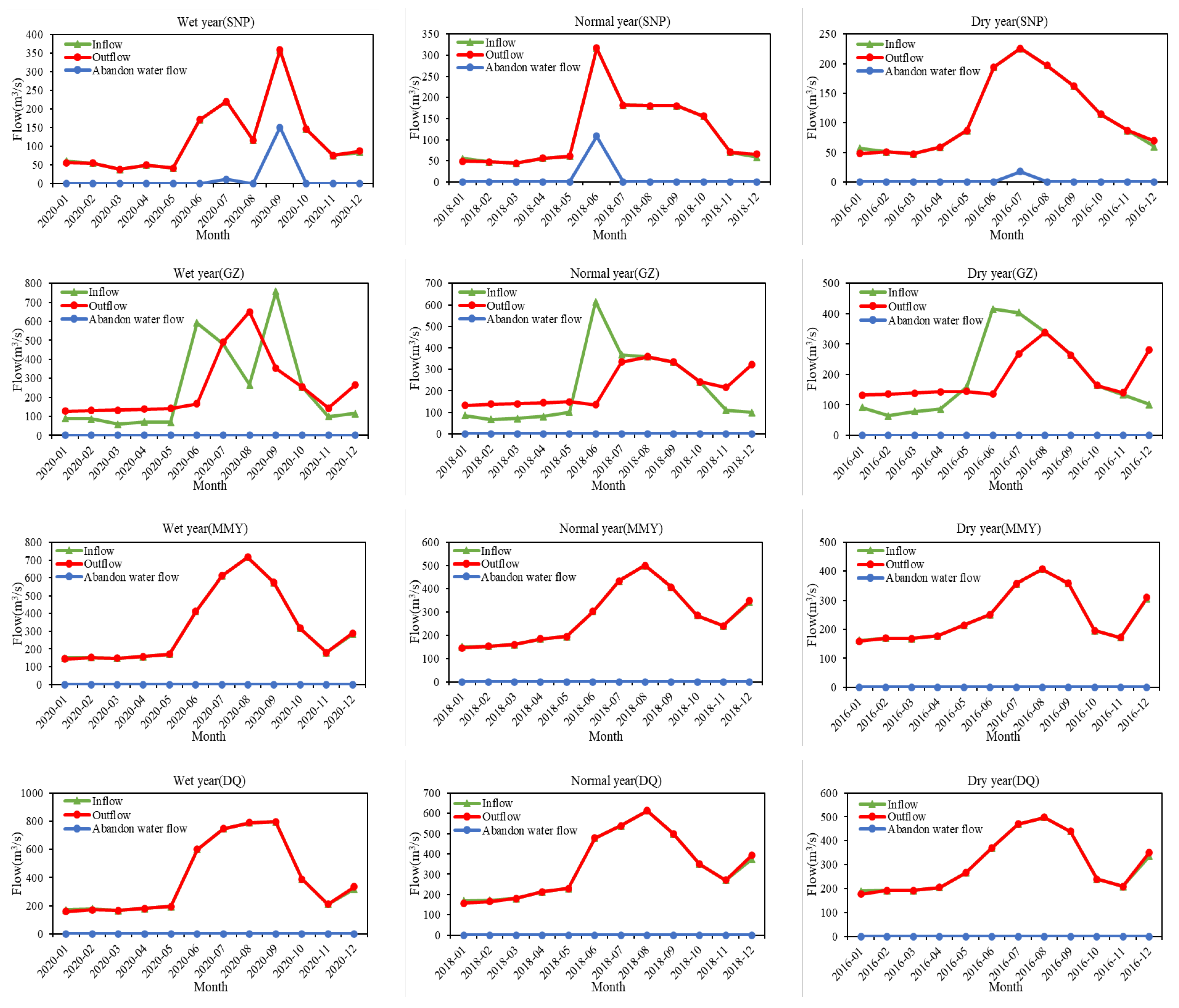
5. Case Study
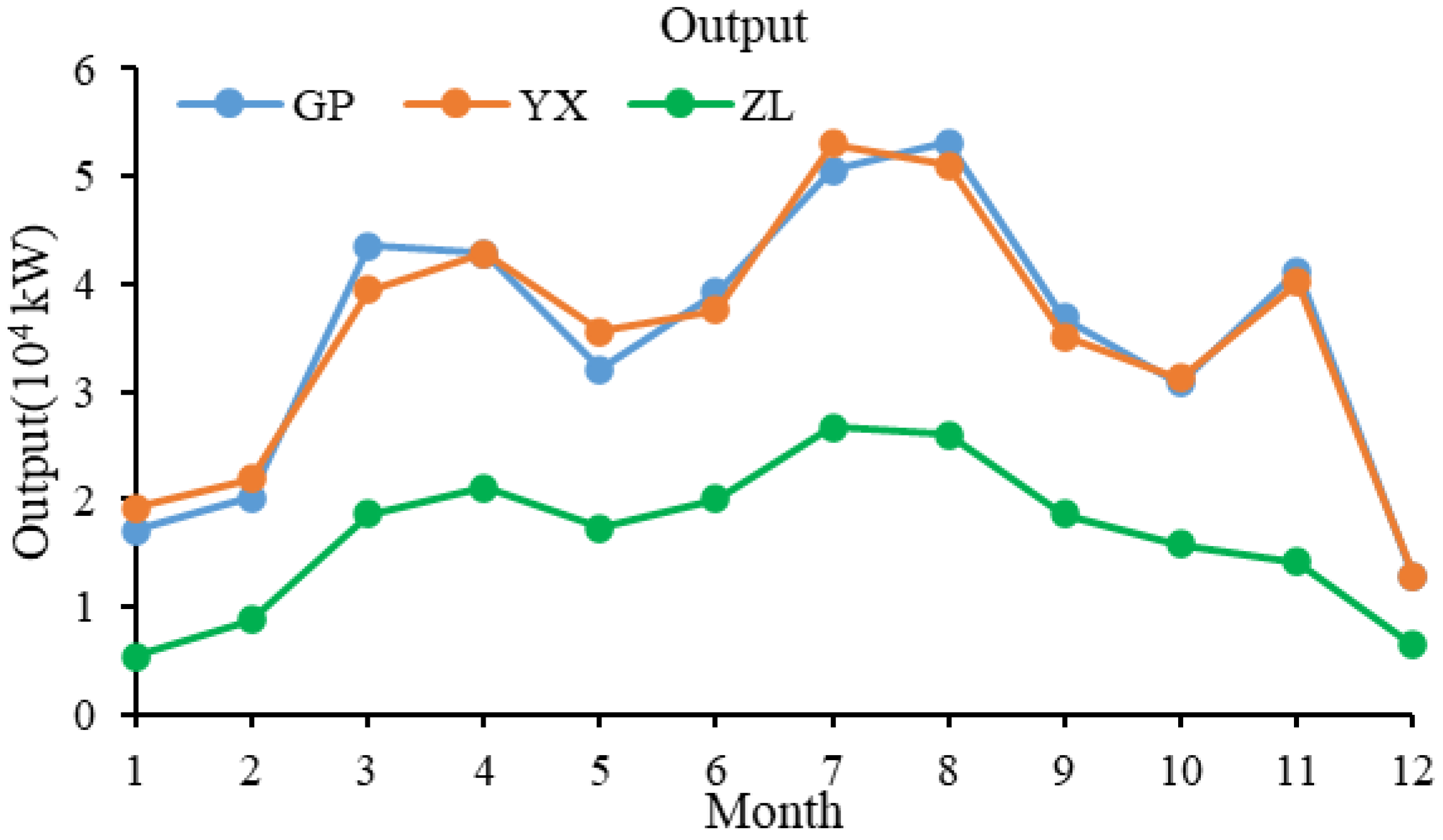
5.1. Engineering Background
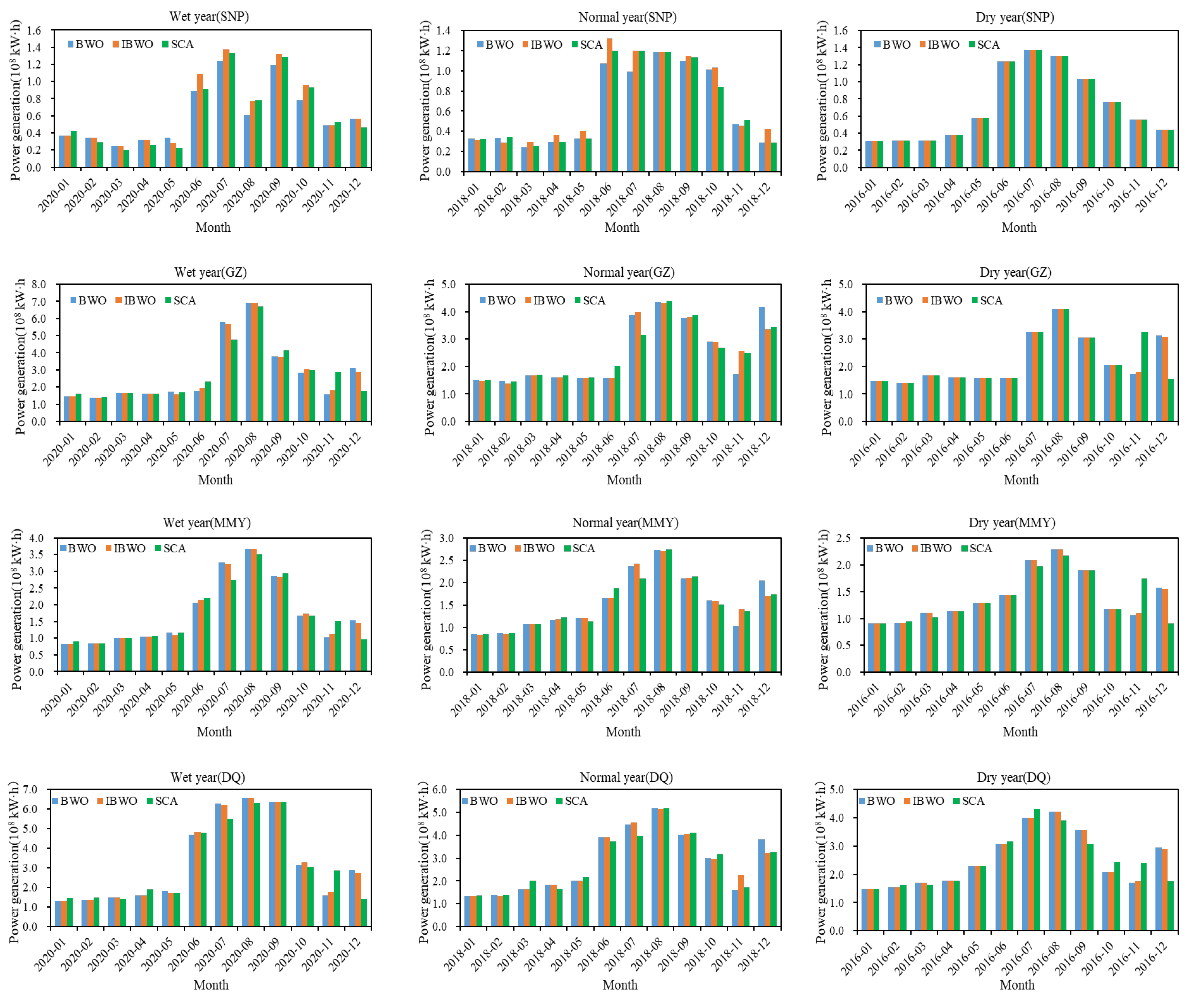
5.2. Statistical Result Comparison
6. Conclusions
Author Contributions
Funding
Data Availability Statement
Acknowledgments
Conflicts of Interest
References
- Ming, B.; Liu, P.; Guo, S.; Zhang, X.; Feng, M.; Wang, X. Optimizing utility-scale photovoltaic power generation for integration into a hydropower reservoir by incorporating long-and short-term operational decisions. Appl. Energy 2017, 204, 432–445. [Google Scholar] [CrossRef]
- Cai, X.; McKinney, D.C.; Lasdon, L.S. Solving nonlinear water management models using a combined genetic algorithm and linear programming approach. Adv. Water Resour. 2001, 24, 667–676. [Google Scholar] [CrossRef]
- Catalo, J.P.S.; Pousinho, H.M.I.; Contreras, J. Optimal hydro scheduling and offering strategies considering price uncertainty and risk management. Energy 2012, 37, 237–244. [Google Scholar] [CrossRef]
- dos Santos Teixeira, A.; Mariño, M.A. Coupled reservoir operation-irrigation scheduling by dynamic programming. J. Irrig. Drain. Eng. 2002, 128, 63–73. [Google Scholar] [CrossRef]
- Feng, Z.; Niu, W.; Cheng, C. Optimization of hydropower reservoirs operation balancing generation benefit and ecological requirement with parallel multi-objective genetic algorithm. Energy 2018, 153, 706–718. [Google Scholar] [CrossRef]
- Yang, T.; Gao, X.; Sorooshian, S.; Li, X. Simulating California reservoir operation using the classification and regression-tree algorithm combined with a shuffled cross-validation scheme. Water Resour. Res. 2016, 52, 1626–1651. [Google Scholar] [CrossRef]
- Jiang, Z.; Duan, J.; Xiao, Y.; He, S. Elite collaborative search algorithm and its application in power generation scheduling optimization of cascade reservoirs. J. Hydrol. 2022, 615, 128684. [Google Scholar] [CrossRef]
- Niu, W.; Feng, Z.; Cheng, C.; Zhou, J. Forecasting daily runoff by extreme learning machine based on quantum-behaved particle swarm optimization. J. Hydrol. Eng. 2018, 23, 04018002. [Google Scholar] [CrossRef]
- Liu, J.; Liu, X.; Wu, Y.; Yang, Z.; Xu, J. Dynamic multi-swarm differential learning Harris Hawks Optimizer and its application to optimal dispatch problem of cascade hydropower stations. Knowl. Based Syst. 2022, 242, 108281. [Google Scholar] [CrossRef]
- Niu, W.; Feng, Z.; Liu, S.; Chen, Y.; Xu, Y.; Zhang, J. Multiple hydropower reservoirs operation by hyperbolic grey wolf optimizer based on elitism selection and adaptive mutation. Water Resour. Manag. 2021, 35, 573–591. [Google Scholar] [CrossRef]
- Nguyen, T.T.; Pham, L.H.; Mohammadi, F.; Kien, L.C. Optimal scheduling of large-scale wind-hydro-thermal systems with fixed-head short-term model. Appl. Sci. 2020, 10, 2964. [Google Scholar] [CrossRef]
- Mantawy, A.H.; Soliman, S.A.; El-Hawary, M.E. An innovative simulated annealing approach to the long-term hydroscheduling problem. Int. J. Electr. Power Energy Syst. 2003, 25, 41–46. [Google Scholar] [CrossRef]
- Niu, W.; Feng, Z.; Liu, S. Multi-strategy gravitational search algorithm for constrained global optimization in coordinative operation of multiple hydropower reservoirs and solar photovoltaic power plants. Appl. Soft Comput. 2021, 107, 107315. [Google Scholar] [CrossRef]
- Tao, Y.; Mo, L.; Yang, Y.; Liu, Z.; Liu, Y.; Liu, T. Optimization of Cascade Reservoir Operation for Power Generation, Based on an Improved Lightning Search Algorithm. Water 2023, 15, 3417. [Google Scholar] [CrossRef]
- Kougias, I.P.; Theodossiou, N.P. Application of the harmony search optimization algorithm for the solution of the multiple dam system scheduling. Optim. Eng. 2013, 14, 331–344. [Google Scholar] [CrossRef]
- Roy, P.K.; Sur, A.; Pradhan, D.K. Optimal short-term hydro-thermal scheduling using quasi-oppositional teaching learning based optimization. Eng. Appl. Artif. Intell. 2013, 26, 2516–2524. [Google Scholar] [CrossRef]
- Hashim, F.A.; Hussien, A.G. Snake Optimizer: A novel meta-heuristic optimization algorithm. Knowl.-Based Syst. 2022, 242, 108320. [Google Scholar] [CrossRef]
- MiarNaeimi, F.; Azizyan, G.; Rashki, M. Horse herd optimization algorithm: A nature-inspired algorithm for high-dimensional optimization problems. Knowl.-Based Syst. 2021, 213, 106711. [Google Scholar] [CrossRef]
- Abdel-Basset, M.; Mohamed, R.; Azeem, S.A.A.; Jameel, M.; Abouhawwash, M. Kepler optimization algorithm: A new metaheuristic algorithm inspired by Kepler’s laws of planetary motion. Knowl. Based Syst. 2023, 268, 110454. [Google Scholar] [CrossRef]
- Nguyen, T.T.; Vo, D.N.; Dinh, B.H. An effectively adaptive selective cuckoo search algorithm for solving three complicated short-term hydrothermal scheduling problems. Energy 2018, 155, 930–956. [Google Scholar] [CrossRef]
- Yin, H.; Wu, F.; Meng, X.; Lin, Y.; Fan, J.; Meng, A. Crisscross optimization based short-term hydrothermal generation scheduling with cascaded reservoirs. Energy 2020, 203, 117822. [Google Scholar] [CrossRef]
- Feng, Z.K.; Liu, S.; Niu, W.J.; Li, S.S.; Wu, H.J.; Wang, J.Y. Ecological operation of cascade hydropower reservoirs by elite-guide gravitational search algorithm with Lévy flight local search and mutation. J. Hydrol. 2020, 581, 124425. [Google Scholar] [CrossRef]
- Niu, W.J.; Feng, Z.K.; Chen, Y.B.; Min, Y.W.; Liu, S.; Li, B.J. Multireservoir system operation optimization by hybrid quantum-behaved particle swarm optimization and heuristic constraint handling technique. J. Hydrol. 2020, 590, 125477. [Google Scholar] [CrossRef]
- Wolpert, D.H.; Macready, W.G. No free lunch theorems for optimization. IEEE Trans. Evol. Comput. 1997, 1, 67–82. [Google Scholar] [CrossRef]
- Zhong, C.; Li, G.; Meng, Z. Beluga whale optimization: A novel nature-inspired metaheuristic algorithm. Knowl. Based Syst. 2022, 251, 109215. [Google Scholar] [CrossRef]
- Yuan, X.; Hu, G.; Zhong, J.; Wei, G. HBWO-JS: Jellyfish search boosted hybrid beluga whale optimization algorithm for engineering applications. J. Comput. Des. Eng. 2023, 10, 1615–1656. [Google Scholar] [CrossRef]
- Hussien, A.G.; Abu Khurma, R.; Alzaqebah, A.; Amin, M.; Hashim, F.A. Novel memetic of beluga whale optimization with self-adaptive exploration–exploitation balance for global optimization and engineering problems. Soft Comput. 2023, 27, 13951–13989. [Google Scholar] [CrossRef]
- Mantegna, R.N. Fast, accurate algorithm for numerical simulation of Levy stable stochastic processes. Phys. Rev. E Stat. Phys. Plasmas Fluids Relat. Interdiscip. 1994, 49, 4677–4683. [Google Scholar] [CrossRef]
- Hu, P.; Pan, J.S.; Chu, S.C. Improved binary grey wolf optimizer and its application for feature selection. Knowl. Based Syst. 2020, 195, 105746. [Google Scholar] [CrossRef]
- Mirjalili, S. SCA: A sine cosine algorithm for solving optimization problems. Knowl. Based Syst. 2016, 96, 120–133. [Google Scholar] [CrossRef]
- Mirjalili, S. Moth-flame optimization algorithm: A novel nature-inspired heuristic paradigm. Knowl. Based Syst. 2015, 89, 228–249. [Google Scholar] [CrossRef]
- Abualigah, L.; Diabat, A.; Mirjalili, S.; Abd Elaziz, M.; Gandomi, A.H. The arithmetic optimization algorithm. Comput. Methods Appl. Mech. Eng. 2021, 376, 113609. [Google Scholar] [CrossRef]
- Mirjalili, S.; Lewis, A. The whale optimization algorithm. Adv. Eng. Softw. 2016, 95, 51–67. [Google Scholar] [CrossRef]
- Ezugwu, A.E.; Agushaka, J.O.; Abualigah, L.; Mirjalili, S.; Gandomi, A.H. Prairie dog optimization algorithm. Neural Comput. Appl. 2022, 34, 20017–20065. [Google Scholar] [CrossRef]
- Abualigah, L.; Abd Elaziz, M.; Sumari, P.; Geem, Z.W.; Gandomi, A.H. Reptile Search Algorithm (RSA): A nature-inspired meta-heuristic optimizer. Expert Syst. Appl. 2022, 191, 116158. [Google Scholar] [CrossRef]
- Arini, F.Y.; Chiewchanwattana, S.; Soomlek, C.; Sunat, K. Joint Opposite Selection (JOS): A premiere joint of selective leading opposition and dynamic opposite enhanced Harris’ hawks optimization for solving single-objective problems. Expert Syst. Appl. 2022, 188, 116001. [Google Scholar] [CrossRef]
- Braik, M.; Hammouri, A.; Atwan, J.; Al-Betar, M.A.; Awadallah, M.A. White Shark Optimizer: A novel bio-inspired meta-heuristic algorithm for global optimization problems. Knowl. Based Syst. 2022, 243, 108457. [Google Scholar] [CrossRef]
- Wang, X.; Virguez, E.; Kern, J.; Chen, L.; Mei, Y.; Patiño-Echeverri, D.; Wang, H. Integrating wind, photovoltaic, and large hydropower during the reservoir refilling period. Energy Convers. Manag. 2019, 198, 111778. [Google Scholar] [CrossRef]
- Zhang, R.; Zhou, J.; Zhang, H.; Liao, X.; Wang, X. Optimal operation of large-scale cascaded hydropower systems in the upper reaches of the Yangtze River, China. J. Water Resour. Plan. Manag. 2014, 140, 480–495. [Google Scholar] [CrossRef]


| Algorithm | Parameter | Value |
|---|---|---|
| SCA | a | 2 |
| MFO | r | [−1, −2] |
| b | 1 | |
| AOA | α | 5 |
| μ | 0.5 | |
| WOA | a | [0, 2] |
| b | 1 | |
| PDO | ρ | 0.1 |
| ε | 2.2204 × 10⁻¹⁶ | |
| Δ | 0.005 | |
| RSA | α | 0.1 |
| β | 0.005 | |
| BWO | [0.1, 0.05] | |
| IBWO | [0.1, 0.05] | |
| P | 0.9 |
| Function | Metrics | SCA | MFO | AOA | WOA | PDO | RSA | BWO | IBWO |
|---|---|---|---|---|---|---|---|---|---|
| F1 | mean | 3.2242E+00 | 1.3352E+03 | 7.6977E-17 | 4.0616E-84 | 0.0000E+00 | 0.0000E+00 | 1.5616E-260 | 0.0000E+00 |
| std | 1.0548E+01 | 4.3426E+03 | 4.2162E-16 | 1.3089E-83 | 0.0000E+00 | 0.0000E+00 | 0.0000E+00 | 0.0000E+00 | |
| rank | 5 | 6 | 4 | 3 | 1 | 1 | 2 | 1 | |
| F2 | mean | 6.1054E-03 | 3.0420E+01 | 0.0000E+00 | 1.0724E-53 | 0.0000E+00 | 0.0000E+00 | 1.2409E-132 | 0.0000E+00 |
| std | 7.7817E-03 | 1.6471E+01 | 0.0000E+00 | 4.7709E-53 | 0.0000E+00 | 0.0000E+00 | 4.0593E-132 | 0.0000E+00 | |
| rank | 4 | 5 | 1 | 3 | 1 | 1 | 2 | 1 | |
| F3 | mean | 2.7574E-04 | 7.4043E-11 | 0.0000E+00 | 2.7967E-125 | 0.0000E+00 | 0.0000E+00 | 1.7939E-268 | 0.0000E+00 |
| std | 1.4679E-03 | 2.2222E-10 | 0.0000E+00 | 1.4117E-124 | 0.0000E+00 | 0.0000E+00 | 0.0000E+00 | 0.0000E+00 | |
| rank | 5 | 4 | 1 | 3 | 1 | 1 | 2 | 1 | |
| F4 | mean | 6.5723E+03 | 1.5910E+04 | 8.0211E-04 | 2.5703E+04 | 0.0000E+00 | 0.0000E+00 | 1.1366E-243 | 0.0000E+00 |
| std | 4.2141E+03 | 1.1468E+04 | 2.3477E-03 | 9.3763E+03 | 0.0000E+00 | 0.0000E+00 | 0.0000E+00 | 0.0000E+00 | |
| rank | 4 | 5 | 3 | 6 | 1 | 1 | 2 | 1 | |
| F5 | mean | 2.9048E+01 | 5.9273E+01 | 2.0937E-02 | 4.1845E+01 | 0.0000E+00 | 0.0000E+00 | 3.3556E-127 | 0.0000E+00 |
| std | 1.0695E+01 | 8.6989E+00 | 2.0075E-02 | 2.9555E+01 | 0.0000E+00 | 0.0000E+00 | 1.7852E-126 | 0.0000E+00 | |
| rank | 4 | 6 | 3 | 5 | 1 | 1 | 2 | 1 | |
| F6 | mean | 9.7224E+03 | 1.2939E+04 | 2.8113E+01 | 2.7359E+01 | 1.5831E+01 | 1.4434E+01 | 5.0851E-07 | 0.0000E+00 |
| std | 3.2669E+04 | 3.0859E+04 | 3.6536E-01 | 3.4013E-01 | 1.3555E+01 | 1.4682E+01 | 8.6442E-07 | 0.0000E+00 | |
| rank | 7 | 8 | 6 | 5 | 4 | 3 | 2 | 1 | |
| F7 | mean | 1.0192E+01 | 2.0349E+03 | 2.8802E+00 | 7.3462E-02 | 2.8800E+00 | 6.6892E+00 | 5.4244E-15 | 0.0000E+00 |
| std | 9.3800E+00 | 5.5346E+03 | 2.5169E-01 | 7.4832E-02 | 1.7797E+00 | 8.3102E-01 | 1.0420E-14 | 0.0000E+00 | |
| rank | 7 | 8 | 5 | 3 | 4 | 6 | 2 | 1 | |
| F8 | mean | 7.1233E-02 | 2.4413E+00 | 4.8053E-05 | 2.4605E-03 | 6.5014E-05 | 8.2912E-05 | 5.4864E-05 | 1.5437E-04 |
| std | 6.0893E-02 | 4.9077E+00 | 4.1995E-05 | 3.1039E-03 | 5.6623E-05 | 9.5413E-05 | 4.8615E-05 | 1.2198E-04 | |
| rank | 7 | 8 | 1 | 6 | 3 | 4 | 2 | 5 | |
| F9 | mean | 2.1605E+01 | 2.9727E+02 | 2.5190E+02 | 4.9563E+02 | 0.0000E+00 | 0.0000E+00 | 2.5765E-229 | 0.0000E+00 |
| std | 1.2379E+01 | 1.0254E+02 | 6.9551E+01 | 1.0795E+02 | 0.0000E+00 | 0.0000E+00 | 0.0000E+00 | 0.0000E+00 | |
| rank | 3 | 5 | 4 | 6 | 1 | 1 | 2 | 1 | |
| F10 | mean | −3.8421E+03 | −8.7436E+03 | −5.5681E+03 | −1.1475E+04 | −3.8941E+03 | −5.4649E+03 | −1.2569E+04 | −1.2569E+04 |
| std | 2.9956E+02 | 8.5520E+02 | 3.7483E+02 | 1.3621E+03 | 3.0733E+02 | 2.3343E+02 | 1.5377E-09 | 1.8501E-12 | |
| rank | 7 | 3 | 4 | 2 | 6 | 5 | 1 | 1 | |
| F11 | mean | 5.4649E+00 | 4.3542E+00 | 0.0000E+00 | 5.1502E-01 | 6.9728E-01 | 0.0000E+00 | 0.0000E+00 | 0.0000E+00 |
| std | 1.6102E+00 | 9.1082E-01 | 0.0000E+00 | 6.2531E-01 | 1.8217E+00 | 0.0000E+00 | 0.0000E+00 | 0.0000E+00 | |
| rank | 5 | 4 | 1 | 2 | 3 | 1 | 1 | 1 | |
| F12 | mean | −5.9748E+02 | −1.0176E+03 | −5.0816E+02 | −1.1170E+03 | −9.3361E+02 | −5.1794E+02 | −1.1750E+03 | −1.1750E+03 |
| std | 3.6289E+01 | 3.5747E+01 | 5.9751E+01 | 8.3461E+01 | 4.2913E+01 | 3.9949E+01 | 4.8559E-12 | 2.2737E-13 | |
| rank | 5 | 3 | 7 | 2 | 4 | 6 | 1 | 1 | |
| F13 | mean | 3.3682E+01 | 1.5923E+02 | 0.0000E+00 | 0.0000E+00 | 0.0000E+00 | 0.0000E+00 | 0.0000E+00 | 0.0000E+00 |
| std | 2.9614E+01 | 3.4366E+01 | 0.0000E+00 | 0.0000E+00 | 0.0000E+00 | 0.0000E+00 | 0.0000E+00 | 0.0000E+00 | |
| rank | 2 | 3 | 1 | 1 | 1 | 1 | 1 | 1 | |
| F14 | mean | 1.1265E+01 | 1.0235E+01 | 4.4409E-16 | 5.0626E-15 | 4.4409E-16 | 4.4409E-16 | 4.4409E-16 | 4.4409E-16 |
| std | 9.4945E+00 | 9.2496E+00 | 0.0000E+00 | 2.4948E-15 | 0.0000E+00 | 0.0000E+00 | 0.0000E+00 | 0.0000E+00 | |
| rank | 4 | 3 | 1 | 2 | 1 | 1 | 1 | 1 | |
| F15 | mean | 8.0157E-01 | 2.1818E+01 | 1.0701E-01 | 2.1114E-02 | 0.0000E+00 | 0.0000E+00 | 0.0000E+00 | 0.0000E+00 |
| std | 2.5551E-01 | 5.1185E+01 | 7.3064E-02 | 4.6353E-02 | 0.0000E+00 | 0.0000E+00 | 0.0000E+00 | 0.0000E+00 | |
| rank | 4 | 5 | 3 | 2 | 1 | 1 | 1 | 1 | |
| F16 | mean | 2.7228E-10 | 1.9924E-12 | 4.7285E-08 | −1.6667E-01 | −1.0000E+00 | −1.0000E+00 | −1.0000E+00 | −1.0000E+00 |
| std | 1.2556E-10 | 3.6208E-12 | 3.4877E-08 | 3.7905E-01 | 0.0000E+00 | 0.0000E+00 | 0.0000E+00 | 0.0000E+00 | |
| rank | 4 | 3 | 5 | 2 | 1 | 1 | 1 | 1 | |
| F17 | mean | 2.0158E+02 | 4.3588E+00 | 4.3839E-01 | 8.6896E-03 | 5.3793E-01 | 1.2737E+00 | 1.8681E-14 | 1.5705E-32 |
| std | 7.9299E+02 | 2.8094E+00 | 5.0238E-02 | 8.7275E-03 | 5.1242E-01 | 3.0668E-01 | 2.8914E-14 | 5.5674E-48 | |
| rank | 8 | 7 | 4 | 3 | 5 | 6 | 2 | 1 | |
| F18 | mean | 1.3525E+04 | 9.5031E+00 | 2.7996E+00 | 2.1295E-01 | 2.8969E+00 | 2.6829E-01 | 9.4598E-14 | 1.3498E-32 |
| std | 3.6220E+04 | 6.5449E+00 | 1.1654E-01 | 1.3747E-01 | 2.8863E-01 | 8.2246E-01 | 1.5943E-13 | 5.5674E-48 | |
| rank | 8 | 7 | 5 | 3 | 6 | 4 | 2 | 1 | |
| F19 | mean | 1.3303E+00 | 1.7882E+00 | 8.6437E+00 | 1.6212E+00 | 5.2960E+00 | 3.0180E+00 | 9.9800E-01 | 2.1653E+00 |
| std | 7.5136E-01 | 1.6468E+00 | 4.3019E+00 | 1.8611E+00 | 4.6418E+00 | 1.7497E+00 | 2.6520E-09 | 3.5616E+00 | |
| rank | 2 | 4 | 8 | 3 | 7 | 6 | 1 | 5 | |
| F20 | mean | 1.0837E-03 | 9.7486E-04 | 1.5746E-02 | 7.2820E-04 | 2.7656E-03 | 1.3767E-03 | 3.2782E-04 | 3.1790E-04 |
| std | 3.2028E-04 | 3.2140E-04 | 2.3789E-02 | 4.7497E-04 | 1.0234E-02 | 6.9838E-04 | 1.6331E-05 | 1.5488E-05 | |
| rank | 5 | 4 | 8 | 3 | 7 | 6 | 2 | 1 | |
| F21 | mean | −1.0316E+00 | −1.0316E+00 | −1.0316E+00 | −1.0316E+00 | −1.0316E+00 | −1.0307E+00 | −1.0315E+00 | −1.0316E+00 |
| std | 2.7246E-05 | 6.7752E-16 | 1.0834E-07 | 2.2169E-10 | 4.0975E-08 | 1.3510E-03 | 1.0661E-04 | 5.1992E-16 | |
| rank | 1 | 1 | 1 | 1 | 1 | 3 | 2 | 1 | |
| F22 | mean | −2.5803E+00 | −7.3070E+00 | −3.9336E+00 | −8.3693E+00 | −5.4930E+00 | −5.0552E+00 | −1.0148E+01 | −1.0153E+01 |
| std | 1.8810E+00 | 3.2042E+00 | 1.2507E+00 | 2.5934E+00 | 2.7533E+00 | 3.2046E-07 | 6.3122E-03 | 5.5785E-15 | |
| rank | 8 | 4 | 7 | 3 | 5 | 6 | 2 | 1 | |
| F23 | mean | −3.9253E+00 | −8.3170E+00 | −4.1836E+00 | −8.8437E+00 | −6.5014E+00 | −5.0877E+00 | −1.0396E+01 | −1.0403E+01 |
| std | 1.8462E+00 | 3.2676E+00 | 1.4766E+00 | 2.6510E+00 | 2.9598E+00 | 9.4738E-07 | 1.1673E-02 | 4.7728E-13 | |
| rank | 8 | 4 | 7 | 3 | 5 | 6 | 2 | 1 | |
| F24 | mean | −4.4769E+00 | −7.8330E+00 | −4.2609E+00 | −8.4461E+00 | −5.4637E+00 | −5.1285E+00 | −1.0529E+01 | −1.0536E+01 |
| std | 1.4970E+00 | 3.6280E+00 | 1.7322E+00 | 3.0951E+00 | 3.1768E+00 | 1.4018E-06 | 1.1849E-02 | 1.7337E-11 | |
| rank | 7 | 4 | 8 | 3 | 5 | 6 | 2 | 1 | |
| mean rank | 5.17 | 4.75 | 4.08 | 3.13 | 3.13 | 3.25 | 1.67 | 1.33 | |
| final ranking | 7 | 6 | 5 | 3 | 3 | 4 | 2 | 1 | |
| Function | Metrics | SCA | MFO | AOA | WOA | PDO | RSA | BWO | IBWO |
|---|---|---|---|---|---|---|---|---|---|
| F1 | mean | 0.0572 | 0.0589 | 0.0478 | 0.0425 | 0.5892 | 0.4929 | 0.0986 | 0.0924 |
| rank | 3 | 4 | 2 | 1 | 8 | 7 | 6 | 5 | |
| F2 | mean | 0.0571 | 0.0605 | 0.0490 | 0.0443 | 0.5791 | 0.4788 | 0.1000 | 0.0926 |
| rank | 3 | 4 | 2 | 1 | 8 | 7 | 6 | 5 | |
| F3 | mean | 0.1059 | 0.1146 | 0.0980 | 0.1011 | 0.6031 | 0.5113 | 0.1468 | 0.1106 |
| rank | 3 | 5 | 1 | 2 | 8 | 7 | 6 | 4 | |
| F4 | mean | 0.1443 | 0.1455 | 0.1336 | 0.1428 | 0.6744 | 0.5745 | 0.1988 | 0.2872 |
| rank | 3 | 4 | 1 | 2 | 8 | 7 | 5 | 6 | |
| F5 | mean | 0.0579 | 0.0587 | 0.0475 | 0.0453 | 0.5740 | 0.4818 | 0.0983 | 0.0890 |
| rank | 3 | 4 | 2 | 1 | 8 | 7 | 6 | 5 | |
| F6 | mean | 0.0673 | 0.0713 | 0.0591 | 0.0612 | 0.5874 | 0.4966 | 0.1114 | 0.1155 |
| rank | 3 | 4 | 1 | 2 | 8 | 7 | 5 | 6 | |
| F7 | mean | 0.0581 | 0.0606 | 0.0470 | 0.0494 | 0.5795 | 0.4878 | 0.0994 | 0.0917 |
| rank | 3 | 4 | 1 | 2 | 8 | 7 | 6 | 5 | |
| F8 | mean | 0.1191 | 0.1203 | 0.1109 | 0.1362 | 0.6073 | 0.5161 | 0.1669 | 0.2308 |
| rank | 2 | 3 | 1 | 4 | 8 | 7 | 5 | 6 | |
| F9 | mean | 0.0714 | 0.0707 | 0.0602 | 0.0572 | 0.5894 | 0.5000 | 0.1128 | 0.1159 |
| rank | 4 | 3 | 2 | 1 | 8 | 7 | 5 | 6 | |
| F10 | mean | 0.0725 | 0.0689 | 0.0605 | 0.0596 | 0.5845 | 0.4945 | 0.1089 | 0.1148 |
| rank | 4 | 3 | 2 | 1 | 8 | 7 | 5 | 6 | |
| F11 | mean | 0.0730 | 0.0694 | 0.0536 | 0.0575 | 0.5871 | 0.4870 | 0.1051 | 0.1045 |
| rank | 4 | 3 | 1 | 2 | 8 | 7 | 6 | 5 | |
| F12 | mean | 0.1291 | 0.1279 | 0.1182 | 0.1272 | 0.6452 | 0.5502 | 0.1798 | 0.2550 |
| rank | 4 | 3 | 1 | 2 | 8 | 7 | 5 | 6 | |
| F13 | mean | 0.0665 | 0.0665 | 0.0479 | 0.0455 | 0.5768 | 0.4830 | 0.0998 | 0.0931 |
| rank | 4 | 3 | 2 | 1 | 8 | 7 | 6 | 5 | |
| F14 | mean | 0.0745 | 0.0720 | 0.0511 | 0.0495 | 0.5839 | 0.4966 | 0.1011 | 0.0981 |
| rank | 4 | 3 | 2 | 1 | 8 | 7 | 6 | 5 | |
| F15 | mean | 0.0780 | 0.0796 | 0.0614 | 0.0602 | 0.5871 | 0.4949 | 0.1105 | 0.1182 |
| rank | 3 | 4 | 2 | 1 | 8 | 7 | 5 | 6 | |
| F16 | mean | 0.0888 | 0.0836 | 0.0704 | 0.0772 | 0.5931 | 0.4991 | 0.1177 | 0.1287 |
| rank | 4 | 3 | 1 | 2 | 8 | 7 | 5 | 6 | |
| F17 | mean | 0.2283 | 0.2320 | 0.2174 | 0.2315 | 0.7426 | 0.6547 | 0.2833 | 0.4700 |
| rank | 2 | 4 | 1 | 3 | 8 | 7 | 5 | 6 | |
| F18 | mean | 0.2359 | 0.2379 | 0.2118 | 0.2365 | 0.7513 | 0.6586 | 0.2871 | 0.4704 |
| rank | 2 | 4 | 1 | 3 | 8 | 7 | 5 | 6 | |
| F19 | mean | 0.2928 | 0.2959 | 0.2928 | 0.3339 | 0.3555 | 0.3217 | 0.3460 | 0.6561 |
| rank | 2 | 3 | 1 | 5 | 7 | 4 | 6 | 8 | |
| F20 | mean | 0.0232 | 0.0244 | 0.0227 | 0.0403 | 0.1085 | 0.0825 | 0.0490 | 0.0635 |
| rank | 2 | 3 | 1 | 4 | 8 | 7 | 5 | 6 | |
| F21 | mean | 0.0223 | 0.0241 | 0.0222 | 0.0388 | 0.0733 | 0.0533 | 0.0467 | 0.0649 |
| rank | 2 | 3 | 1 | 4 | 8 | 6 | 5 | 7 | |
| F22 | mean | 0.0304 | 0.0318 | 0.0300 | 0.0511 | 0.1201 | 0.0909 | 0.0580 | 0.0808 |
| rank | 2 | 3 | 1 | 4 | 8 | 7 | 5 | 6 | |
| F23 | mean | 0.0336 | 0.0371 | 0.0337 | 0.0570 | 0.1254 | 0.0978 | 0.0622 | 0.0889 |
| rank | 1 | 3 | 2 | 4 | 8 | 7 | 5 | 6 | |
| F24 | mean | 0.0400 | 0.0408 | 0.0379 | 0.0607 | 0.1285 | 0.1019 | 0.0670 | 0.0997 |
| rank | 2 | 3 | 1 | 4 | 8 | 7 | 5 | 6 | |
| mean rank | 2.88 | 3.46 | 1.38 | 2.38 | 7.96 | 6.83 | 5.38 | 5.75 | |
| final ranking | 3 | 4 | 1 | 2 | 8 | 7 | 5 | 6 | |
| Function | Metrics | SCA | MFO | AOA | WOA | PDO | RSA | BWO | IBWO |
|---|---|---|---|---|---|---|---|---|---|
| F1 | mean | 1.21E+10 | 8.26E+09 | 4.16E+10 | 2.56E+06 | 3.61E+10 | 4.23E+10 | 4.43E+10 | 1.06E+05 |
| std | 1.87E+09 | 5.71E+09 | 5.20E+09 | 2.07E+06 | 9.65E+09 | 5.49E+09 | 3.89E+09 | 5.22E+04 | |
| rank | 4 | 3 | 6 | 2 | 5 | 7 | 8 | 1 | |
| F2 | NA | NA | NA | NA | NA | NA | NA | NA | |
| F3 | mean | 3.54E+04 | 8.76E+04 | 7.58E+04 | 1.43E+05 | 6.45E+04 | 7.15E+04 | 7.14E+04 | 6.71E+03 |
| std | 8.25E+03 | 5.44E+04 | 7.67E+03 | 4.76E+04 | 8.45E+03 | 8.83E+03 | 4.86E+03 | 2.56E+03 | |
| rank | 2 | 7 | 6 | 8 | 3 | 5 | 4 | 1 | |
| F4 | mean | 1.38E+03 | 9.04E+02 | 9.16E+03 | 5.51E+02 | 7.60E+03 | 8.31E+03 | 9.67E+03 | 5.00E+02 |
| std | 2.62E+02 | 3.67E+02 | 1.99E+03 | 4.87E+01 | 3.46E+03 | 2.27E+03 | 1.28E+03 | 2.47E+01 | |
| rank | 4 | 3 | 7 | 2 | 5 | 6 | 8 | 1 | |
| F5 | mean | 7.77E+02 | 6.99E+02 | 8.09E+02 | 7.97E+02 | 8.25E+02 | 8.93E+02 | 8.92E+02 | 7.03E+02 |
| std | 2.42E+01 | 4.67E+01 | 3.92E+01 | 7.18E+01 | 5.08E+01 | 3.11E+01 | 1.63E+01 | 5.09E+01 | |
| rank | 3 | 1 | 5 | 4 | 6 | 8 | 7 | 2 | |
| F6 | mean | 6.48E+02 | 6.34E+02 | 6.64E+02 | 6.67E+02 | 6.78E+02 | 6.79E+02 | 6.82E+02 | 6.10E+02 |
| std | 5.17E+00 | 1.06E+01 | 6.33E+00 | 8.73E+00 | 9.65E+00 | 4.45E+00 | 5.96E+00 | 8.97E+00 | |
| rank | 3 | 2 | 4 | 5 | 6 | 7 | 8 | 1 | |
| F7 | mean | 1.12E+03 | 1.06E+03 | 1.31E+03 | 1.26E+03 | 1.39E+03 | 1.35E+03 | 1.34E+03 | 1.10E+03 |
| std | 3.27E+01 | 1.64E+02 | 3.77E+01 | 7.94E+01 | 1.66E+02 | 4.58E+01 | 2.79E+01 | 8.81E+01 | |
| rank | 3 | 1 | 5 | 4 | 8 | 7 | 6 | 2 | |
| F8 | mean | 1.05E+03 | 9.93E+02 | 1.03E+03 | 1.01E+03 | 1.06E+03 | 1.12E+03 | 1.12E+03 | 9.43E+02 |
| std | 2.24E+01 | 5.24E+01 | 3.01E+01 | 5.61E+01 | 6.11E+01 | 1.38E+01 | 1.44E+01 | 2.56E+01 | |
| rank | 5 | 2 | 4 | 3 | 6 | 8 | 7 | 1 | |
| F9 | mean | 5.03E+03 | 6.46E+03 | 5.98E+03 | 8.04E+03 | 7.16E+03 | 9.14E+03 | 9.96E+03 | 4.92E+03 |
| std | 8.77E+02 | 2.24E+03 | 7.90E+02 | 2.68E+03 | 2.29E+03 | 8.37E+02 | 8.23E+02 | 9.09E+02 | |
| rank | 2 | 4 | 3 | 6 | 5 | 7 | 8 | 1 | |
| F10 | mean | 8.08E+03 | 5.08E+03 | 6.51E+03 | 6.18E+03 | 7.78E+03 | 7.76E+03 | 8.22E+03 | 4.69E+03 |
| std | 3.60E+02 | 8.61E+02 | 4.95E+02 | 7.86E+02 | 5.15E+02 | 3.45E+02 | 2.66E+02 | 6.44E+02 | |
| rank | 7 | 2 | 4 | 3 | 6 | 5 | 8 | 1 | |
| F11 | mean | 2.23E+03 | 3.60E+03 | 3.35E+03 | 1.51E+03 | 7.58E+03 | 6.69E+03 | 5.37E+03 | 1.21E+03 |
| std | 4.76E+02 | 2.85E+03 | 9.53E+02 | 1.77E+02 | 2.95E+03 | 1.22E+03 | 7.39E+02 | 4.37E+01 | |
| rank | 3 | 5 | 4 | 2 | 8 | 7 | 6 | 1 | |
| F12 | mean | 1.15E+09 | 1.87E+08 | 8.48E+09 | 5.33E+07 | 8.65E+09 | 1.27E+10 | 7.49E+09 | 2.59E+06 |
| std | 2.80E+08 | 5.18E+08 | 2.64E+09 | 3.00E+07 | 3.02E+09 | 3.47E+09 | 1.63E+09 | 1.81E+06 | |
| rank | 4 | 3 | 6 | 2 | 7 | 8 | 5 | 1 | |
| F13 | mean | 4.07E+08 | 9.94E+06 | 4.06E+04 | 1.40E+05 | 4.96E+09 | 8.58E+09 | 4.03E+09 | 2.63E+04 |
| std | 1.58E+08 | 2.47E+07 | 1.38E+04 | 8.08E+04 | 1.68E+09 | 4.18E+09 | 1.51E+09 | 4.09E+04 | |
| rank | 5 | 4 | 2 | 3 | 7 | 8 | 6 | 1 | |
| F14 | mean | 1.58E+05 | 3.00E+05 | 5.50E+04 | 9.19E+05 | 2.37E+06 | 2.94E+06 | 1.13E+06 | 1.92E+05 |
| std | 1.07E+05 | 1.19E+06 | 4.84E+04 | 8.32E+05 | 1.84E+06 | 1.84E+06 | 5.16E+05 | 1.50E+05 | |
| rank | 2 | 4 | 1 | 5 | 7 | 8 | 6 | 3 | |
| F15 | mean | 1.43E+07 | 6.39E+04 | 2.45E+04 | 7.96E+04 | 9.99E+07 | 5.06E+08 | 1.05E+08 | 1.02E+04 |
| std | 1.39E+07 | 6.89E+04 | 1.16E+04 | 6.70E+04 | 1.21E+08 | 1.45E+08 | 4.66E+07 | 1.04E+04 | |
| rank | 5 | 3 | 2 | 4 | 6 | 8 | 7 | 1 | |
| F16 | mean | 3.65E+03 | 3.12E+03 | 3.95E+03 | 3.60E+03 | 4.59E+03 | 4.66E+03 | 4.93E+03 | 2.65E+03 |
| std | 1.82E+02 | 3.97E+02 | 6.44E+02 | 4.25E+02 | 4.73E+02 | 5.34E+02 | 2.30E+02 | 3.43E+02 | |
| rank | 4 | 2 | 5 | 3 | 6 | 7 | 8 | 1 | |
| F17 | mean | 2.40E+03 | 2.58E+03 | 2.78E+03 | 2.49E+03 | 3.07E+03 | 4.12E+03 | 3.34E+03 | 2.31E+03 |
| std | 1.39E+02 | 2.60E+02 | 2.53E+02 | 2.98E+02 | 3.71E+02 | 1.84E+03 | 2.68E+02 | 2.51E+02 | |
| rank | 2 | 4 | 5 | 3 | 6 | 8 | 7 | 1 | |
| F18 | mean | 3.52E+06 | 1.48E+06 | 1.24E+06 | 1.93E+06 | 1.24E+07 | 4.09E+07 | 1.52E+07 | 1.20E+06 |
| std | 2.67E+06 | 3.24E+06 | 1.43E+06 | 1.98E+06 | 1.14E+07 | 3.28E+07 | 1.09E+07 | 1.46E+06 | |
| rank | 5 | 3 | 2 | 4 | 6 | 8 | 7 | 1 | |
| F19 | mean | 2.06E+07 | 8.91E+06 | 1.06E+06 | 2.19E+06 | 2.67E+08 | 5.01E+08 | 1.64E+08 | 1.58E+04 |
| std | 1.17E+07 | 3.50E+07 | 1.22E+05 | 1.71E+06 | 2.05E+08 | 6.88E+08 | 7.95E+07 | 1.71E+04 | |
| rank | 5 | 4 | 2 | 3 | 7 | 8 | 6 | 1 | |
| F20 | mean | 2.59E+03 | 2.67E+03 | 2.76E+03 | 2.77E+03 | 2.83E+03 | 2.88E+03 | 2.80E+03 | 2.50E+03 |
| std | 1.24E+02 | 2.54E+02 | 1.99E+02 | 1.93E+02 | 1.22E+02 | 1.08E+02 | 1.01E+02 | 1.95E+02 | |
| rank | 2 | 3 | 4 | 5 | 7 | 8 | 6 | 1 | |
| F21 | mean | 2.55E+03 | 2.49E+03 | 2.61E+03 | 2.58E+03 | 2.67E+03 | 2.66E+03 | 2.68E+03 | 2.48E+03 |
| std | 2.26E+01 | 4.32E+01 | 3.91E+01 | 5.01E+01 | 7.68E+01 | 3.49E+01 | 3.03E+01 | 8.89E+01 | |
| rank | 3 | 2 | 5 | 4 | 7 | 6 | 8 | 1 | |
| F22 | mean | 8.43E+03 | 6.26E+03 | 7.88E+03 | 6.91E+03 | 8.41E+03 | 7.96E+03 | 7.86E+03 | 4.91E+03 |
| std | 2.20E+03 | 1.73E+03 | 8.76E+02 | 1.91E+03 | 1.31E+03 | 1.03E+03 | 4.95E+02 | 2.06E+03 | |
| rank | 8 | 2 | 5 | 3 | 7 | 6 | 4 | 1 | |
| F23 | mean | 2.99E+03 | 2.82E+03 | 3.41E+03 | 3.04E+03 | 3.29E+03 | 3.26E+03 | 3.23E+03 | 2.88E+03 |
| std | 2.42E+01 | 2.73E+01 | 1.74E+02 | 9.07E+01 | 7.30E+01 | 1.18E+02 | 3.41E+01 | 6.71E+01 | |
| rank | 3 | 1 | 8 | 4 | 7 | 6 | 5 | 2 | |
| F24 | mean | 3.16E+03 | 2.97E+03 | 3.75E+03 | 3.17E+03 | 3.38E+03 | 3.35E+03 | 3.45E+03 | 3.16E+03 |
| std | 2.97E+01 | 2.76E+01 | 1.63E+02 | 9.65E+01 | 7.12E+01 | 1.02E+02 | 5.88E+01 | 8.71E+01 | |
| rank | 2 | 1 | 7 | 3 | 5 | 4 | 6 | 2 | |
| F25 | mean | 3.20E+03 | 3.31E+03 | 4.44E+03 | 2.95E+03 | 4.39E+03 | 4.49E+03 | 4.17E+03 | 2.90E+03 |
| std | 7.91E+01 | 4.37E+02 | 5.54E+02 | 3.31E+01 | 6.34E+02 | 5.81E+02 | 1.25E+02 | 1.99E+01 | |
| rank | 3 | 4 | 7 | 2 | 6 | 8 | 5 | 1 | |
| F26 | mean | 6.84E+03 | 5.79E+03 | 9.76E+03 | 7.61E+03 | 9.06E+03 | 9.82E+03 | 9.72E+03 | 6.11E+03 |
| std | 4.82E+02 | 4.03E+02 | 1.02E+03 | 1.29E+03 | 1.14E+03 | 1.10E+03 | 5.46E+02 | 7.51E+02 | |
| rank | 3 | 1 | 7 | 4 | 5 | 8 | 6 | 2 | |
| F27 | mean | 3.40E+03 | 3.25E+03 | 4.24E+03 | 3.36E+03 | 3.64E+03 | 3.72E+03 | 3.76E+03 | 3.27E+03 |
| std | 4.15E+01 | 2.15E+01 | 2.90E+02 | 1.02E+02 | 8.03E+01 | 3.59E+02 | 9.74E+01 | 2.35E+01 | |
| rank | 4 | 1 | 8 | 3 | 5 | 6 | 7 | 2 | |
| F28 | mean | 3.79E+03 | 4.13E+03 | 6.07E+03 | 3.30E+03 | 5.46E+03 | 6.05E+03 | 5.87E+03 | 3.23E+03 |
| std | 1.11E+02 | 7.18E+02 | 8.61E+02 | 4.91E+01 | 7.46E+02 | 7.57E+02 | 2.29E+02 | 2.27E+01 | |
| rank | 3 | 4 | 8 | 2 | 5 | 7 | 6 | 1 | |
| F29 | mean | 4.65E+03 | 4.01E+03 | 5.87E+03 | 4.95E+03 | 5.68E+03 | 5.82E+03 | 6.06E+03 | 3.89E+03 |
| std | 2.03E+02 | 2.39E+02 | 6.74E+02 | 5.00E+02 | 4.51E+02 | 7.73E+02 | 4.19E+02 | 2.83E+02 | |
| rank | 3 | 2 | 7 | 4 | 5 | 6 | 8 | 1 | |
| F30 | mean | 7.14E+07 | 4.15E+05 | 2.17E+08 | 8.90E+06 | 8.82E+08 | 2.31E+09 | 5.46E+08 | 1.21E+04 |
| std | 2.07E+07 | 5.90E+05 | 7.02E+08 | 6.51E+06 | 4.29E+08 | 9.85E+08 | 2.08E+08 | 4.65E+03 | |
| rank | 4 | 2 | 5 | 3 | 7 | 8 | 6 | 1 | |
| mean rank | 3.66 | 2.76 | 4.97 | 3.55 | 6.07 | 7.00 | 6.52 | 1.28 | |
| final ranking | 4 | 2 | 5 | 3 | 6 | 8 | 7 | 1 | |
| Power Station | Type | Installed Capacity (MW) | Normal Water Level (m) | Dead Water Level (m) | Maximum Power Generation Flow (m3/s) | Minimum Generation Flow (m3/s) | Minimum Discharge Flow (m3/s) | Maximum Output (104 kw) | Minimum Output (104 kw) |
|---|---|---|---|---|---|---|---|---|---|
| SNP | hydropower reservoir | 185.5 | 885 | 865 | 208.42 | 0 | 7 | 18.55 | 2.042 |
| GZ | hydropower reservoir | 1040 | 745 | 691 | 866 | 0 | 27.6 | 104 | 18.02 |
| MMY | hydropower reservoir | 558 | 585 | 580 | 923.5 | 0 | 31 | 55.8 | 8.73 |
| DQ | hydropower reservoir | 880 | 490 | 483 | 917.2 | 0 | 50 | 88 | 17.2 |
| GP | photovoltaic power plant | 300 | — | — | — | — | — | 30 | — |
| YX | photovoltaic power plant | 300 | — | — | — | — | — | 30 | — |
| ZL | photovoltaic power plant | 150 | — | — | — | — | — | 15 | — |
| Runoff | Algorithm | Average Value | Best | Worst | Standard Deviation |
|---|---|---|---|---|---|
| Wet year | BWO | 100.26 | 101.12 | 99.23 | 0.50 |
| IBWO | 101.83 | 101.94 | 101.74 | 0.09 | |
| SCA | 99.32 | 99.88 | 98.62 | 0.31 | |
| Normal year | BWO | 90.54 | 90.70 | 90.38 | 0.09 |
| IBWO | 91.45 | 91.49 | 91.44 | 0.02 | |
| SCA | 89.67 | 90.30 | 89.16 | 0.28 | |
| Dry year | BWO | 82.43 | 82.43 | 82.43 | 0 |
| IBWO | 82.43 | 82.43 | 82.43 | 0 | |
| SCA | 81.11 | 81.54 | 80.84 | 0.23 |
Disclaimer/Publisher’s Note: The statements, opinions and data contained in all publications are solely those of the individual author(s) and contributor(s) and not of MDPI and/or the editor(s). MDPI and/or the editor(s) disclaim responsibility for any injury to people or property resulting from any ideas, methods, instructions or products referred to in the content. |
© 2025 by the authors. Licensee MDPI, Basel, Switzerland. This article is an open access article distributed under the terms and conditions of the Creative Commons Attribution (CC BY) license (https://creativecommons.org/licenses/by/4.0/).
Share and Cite
Yuan, X.; Qin, H.; Cao, W.; Zhang, T.; Niu, X. Optimal Scheduling Study of Hydro–Solar Complementary System Based on Improved Beluga Whale Algorithm. Water 2025, 17, 878. https://doi.org/10.3390/w17060878
Yuan X, Qin H, Cao W, Zhang T, Niu X. Optimal Scheduling Study of Hydro–Solar Complementary System Based on Improved Beluga Whale Algorithm. Water. 2025; 17(6):878. https://doi.org/10.3390/w17060878
Chicago/Turabian StyleYuan, Xiaofeng, Hui Qin, Wei Cao, Taiheng Zhang, and Xinqiang Niu. 2025. "Optimal Scheduling Study of Hydro–Solar Complementary System Based on Improved Beluga Whale Algorithm" Water 17, no. 6: 878. https://doi.org/10.3390/w17060878
APA StyleYuan, X., Qin, H., Cao, W., Zhang, T., & Niu, X. (2025). Optimal Scheduling Study of Hydro–Solar Complementary System Based on Improved Beluga Whale Algorithm. Water, 17(6), 878. https://doi.org/10.3390/w17060878