Article

Slope Stability Analysis Considering Degradation of Soil Properties Induced by Intermittent Rainfall

School of Civil Engineering, Qingdao University of Technology, Qingdao 266033, China
*
Author to whom correspondence should be addressed.
Water 2025, 17(6), 814; https://doi.org/10.3390/w17060814
Submission received: 5 February 2025 / Revised: 9 March 2025 / Accepted: 11 March 2025 / Published: 12 March 2025

Abstract

:
This paper aims to emphasize the importance of considering the degradation of soil properties induced by intermittent rainfall infiltration in the slope stability analysis of unsaturated soils. A simplified linear degradation model and an exponential degradation model, which are characterized by degradation rate and maximum degradation degree, are used to determine the degradation coefficient at specific time steps within the intermittent rainfall. The proposed simplified linear degradation model is implemented through the commercial software package, Geo-studio 2018, specifically the Seep/w and Slope/w modules. The incorporation of soil degradation into the slope stability analysis is justified via comparisons against an example on the Geo-studio website. It is found that the number of sub-rainfalls exerts a significant influence on the minimum Factor of Safety (FoS) of the unsaturated soil slope stability, whereas the effect of rainfall intervals on the minimum FoS at the end of each sub-rainfall is trivial. The degradation of soil properties induced by intermittent rainfall infiltration can be properly simulated by the proposed simplified linear and nonlinear degradation models. It must be noted that decision making on early warnings can be different even for moderate rainfall with and without consideration of the degradation of soil properties.

1. Introduction

Arising from global climate change, extreme rainfall incidents are observed in geotechnical slope engineering [1,2,3,4,5,6,7]. Rainfall may deteriorate slope stability and, further, lead to landslides, avalanches and other undesirable consequences on slopes, which pose great threats to residents and infrastructure [8,9]. Therefore, a comprehensive study of the effect of rainfall on slope stability is necessary for sustainable geotechnical engineering.
Many scholars worldwide have been committed to investigating the influence of rainfall on slope stability. A conceptual model was developed to deal with rainfall-induced shallow landslides with a wide range of parameters, and it was found that the most significant influencing factor in regional landslides is the initial water content, followed by rainfall duration and intensity [10]. The effects of rainfall intensity, rainfall pattern and rainfall duration on the slope stability were investigated, and it was demonstrated that rainfall intensities exhibit a significant influence on the slope failure mechanism [11,12,13]. For example, rainfall with lower intensity tends to trigger deep landslides, whereas higher-intensity rainfall leads to shallow landslides. The variation of the failure mechanism from deep to shallow landslides is dependent on the variation in the water content within the slope. Since higher-intensity rainfall leads to a rapid increase in water content within the surficial and shallower portion of the slope, a shallow landslide is likely to be observed [14]. The slope stability is more rapidly deteriorated and landslides are observed earlier under higher rainfall intensity [15]. Furthermore, the rainfall pattern, rainfall duration, slope geometry and slope geology also affect slope stability under rainfall conditions. For example, steep slopes are more prone to landslides under rainfall conditions, as compared to flat slopes [16,17,18,19,20]. The vegetation and groundwater level are also important factors affecting slope stability under rainfall conditions [21,22,23]. It is noticed that the effect of the root system of vegetation is to reduce the scouring effect of runoff generated by rainfall on slopes. Rainfall infiltration leads to changes in the groundwater level and the soil’s degree of saturation within the slope and, finally, deteriorates the slope stability.
Apart from the aforementioned factors, another important and straightforward factor influencing slope stability under rainfall conditions is the degradation in shear strength parameters caused by rainfall infiltration. The factor of safety (FoS) of a highway slope was estimated using the finite element method (FEM), and it was revealed that extreme rainfall tends to reduce the soil shear strength, thereby enhancing the probability of landslides [24]. In situ borehole shear tests on expansive soils with different degrees of saturation were conducted, and the results provide insight into the shear strength characteristics of expansive soils under rainfall conditions [25]. The stability of unsaturated loess slopes was evaluated considering the effect of wetting–drying cycles, and it was concluded that the slope stability decreases with the increase in volumetric water content [26]. It is intuitively conceived that within the duration of rainfall, the time-dependent variation of the water content of soils within the slope results in dynamic changes in the degree of saturation and, finally, leads to alternations in shear strength parameters (e.g., cohesion and internal friction angle). To address this variation of the saturation degree of soils in slope stability, 1-D and 2-D rainfall infiltration models were established, and it was demonstrated that with the increase in rainfall duration and rainfall intensity, the cohesion and internal friction angle of the soil decrease, subsequently leading to a decrease in slope stability [27]. Direct shear tests were performed to study the effect of water content on soil shear strength parameters, and this effect was subsequently incorporated into a slope stability analysis. It was manifested that ignoring the effect of water content on the shear strength parameters tends to overestimate the stability of slopes [28]. The degradation of soil properties caused by repeated variations in water level was considered in a stability analysis of upstream and downstream dam slopes [29].
Previous studies have revealed the importance of accounting for the degradation of soil cohesion and internal friction angle during rainfall, and constant and instantaneous degradation models have been developed in [29]. Li et al [29] assumed that repeated immersion in water would lead to an overall degradation of soil parameters. Actually, the intermittent rainfall pattern leads to the re-infiltration of rainwater into soils instead of sustained infiltration. This re-infiltration results in the degradation of soil properties in relation to the number of cycles during which the soil is exposed to rainfall infiltration. As a result, the use of a degradation model that varies with the number of re-infiltrations in slope stability analysis is warranted. Therefore, how to simulate the degradation of cohesion and internal friction angle with the number of re-infiltrations remains an unresolved issue.
In this paper, the basic theory of the seepage and stability analysis of unsaturated soil slopes is first briefly introduced. Next, the proposed methodology is described in detail and illustrated with an existing example from the Geo-studio website, emphasizing the effects of rainfall intensity, rainfall interval time and parameter degradation on the factor of safety (FoS). Finally, conclusions are drawn.

2. Fundamental Theories and Degradation Model

2.1. Theory of Seepage in Unsaturated Soils

The seepage of water within unsaturated soils is governed by generalized Darcy’s Law, Richard’s equation and continuity of water flow. On one hand, the generalized Darcy’s law articulates the relationship between water flow velocity and hydraulic gradient. On the other hand, Richard’s equation delineates how the flow velocity varies with the volumetric water content [30]. Finally, the continuity of water flow implies that the difference between the outflow and inflow of water into a soil element at specific time step equals the soil element’s water storage. Therefore, the general governing differential equation of water seepage within unsaturated soils can be expressed as
θ ( h ) t = θ x i K ( h ) h x j
where θ is the volumetric water content; t is time; h is the pore water pressure head; xi is the spatial coordinates using Einstein’s summation convention; and K is the permeability coefficient of soil, and it varies with h in unsaturated soil.
The relationship between θ and pressure head (i.e., θ(h) in Equation (1)) in unsaturated soils can be properly modeled by a soil water characteristic curve (SWCC). The model proposed by Van Genuchten (1980) is used in this paper [31]:
θ θ r θ s θ r = S e = 1 1 + α μ a μ w n m
where θs is the saturated water content; θr is the residual water content; Se is the effective saturation; a, m and n are the fitting parameters of the model, and m = 1 − 1/n; μa is the pore air pressure; μw is the pore water pressure.
In unsaturated soils, the permeability coefficient K hinges on h, and it is often determined as K = Kr × Ks, where Ks is the saturated permeability coefficient, and Kr is the relative permeability coefficient that varies with h. The relationship between K and h can be determined either by measurements or by using empirical models. For example, the Mualem model is often used in conjunction with the SWCC model described above and is expressed as [32]
K ( h ) = K s S e 1 / 2 1 ( 1 S e 1 / m ) m 2
The analytical solution to Equation (1) cannot be easily obtained, since the control equation is nonlinear. An alternative tool, FEM simulation, is widely employed to determine the hydraulic response of unsaturated soil owing to rainfall infiltration. For seepage analysis, boundary conditions and initial conditions are required in addition to the controlling equations. Seep/w module is used to perform seepage analysis within unsaturated soils and the obtained results are used in the slope stability analysis.

2.2. Shear Strength of Unsaturated Soils

The shear strength of unsaturated soils differs from that of saturated soil owing to the existence of matric suction, which is defined as [33]
δ = μ a μ w
where δ is the matric suction. The shear strength of unsaturated soils is determined in this study by the following equation [34]:
τ f = c + σ μ a tan φ + μ a μ w θ θ r θ s θ r tan φ
where τf is the shear strength; c′ is the effective cohesion for the fully saturated soil; φ′ is the effective friction angle for the fully saturated soil; and σ is the total normal stress.
Equation (5) is implemented into the stability analysis for unsaturated soil slope in Slope/w, where the FoS of the slope can be calculated using the circular traditional limit equilibrium method. In this study, circular slip surface and simplified Bishop method are adopted based on two reasons. The first reason is that noncircular slip is really necessitated for slope scenarios with predominant controlling surfaces, like inter-seams, fissures, joints, which are often observed for rock slopes. The second reason is that failure to converge is always noticed with noncircular slip surfaces, which is more likely to violate the assumptions used in limit equilibrium. As a result, in view of the current scope, the stability analysis for unsaturated soil slope utilizes circular slip surface and simplified Bishop method.

2.3. Degradation of Soil Properties for Unsaturated Soils Under Intermittent Rainfall

The interaction between hydraulic parameters (e.g., rainfall intensity, permeability) and mechanical properties of the soil (e.g., cohesion, internal friction angle) is crucial in slope stability analysis [35,36,37]. As described in introduction section, the degradation of soil properties may be induced by intermittent rainfall. Let Tri denote the ith rainfall duration, and Tei the ith time interval between ith and i + 1th rainfall. Only cohesion and internal friction angle have the potential to be degraded in this study. Before the slope stability analysis, site characterization and laboratory tests are conducted to determine the original cohesion and internal friction angle, denoted by c0 and φ0.

2.3.1. Simplified Linear Degradation Model

The simplified linear degradation model is adopted in this study as an illustration:
D = 1.0                                                         i b 1.0 k i b                   b < i E D min                                                   i > E
where D is the degradation coefficient, D = 1.0 means no degradation of soil properties, i is the sequential number of sub-rainfalls within one intermittent rainfall. The degraded cohesion and internal friction angle are denoted by cD = Dc0 and φD = 0, respectively. It is assumed in this study that cohesion and internal friction angle have exactly the same degradation coefficient. b is the bth sub-rainfall with duration Trb. E is the Eth sub-rainfall with duration TrE. Dmin is the minimum degradation coefficient indicating the maximum degradation degree. k is the coefficient describing the degradation rate. Three independent parameters, Dmin, b and E, can be determined by laboratory test and the dependent parameter k can be determined. It is noted that specific degradation model can be implemented into the proposed method. The use of simplified linear degradation model aims to emphasize the importance of considering degradation in slope stability analysis under intermittent rainfall.

2.3.2. Nonlinear Degradation Model

Nonlinear characteristics of soil behavior, including the nonlinear Mohr–Coulomb failure criterion, are essential in analyzing slope stability [38]. Previous studies have indicated that the degradation of soil parameters is not necessarily linear [39,40,41]. The degradation of cohesion or internal friction angle generally exhibits a negative exponential correlation with the number of water infiltrations [42]. Therefore, a nonlinear degradation model, as shown in Equation (7), is proposed to facilitate the comparison between linear and nonlinear degradation models.
D = 1.0                                       i b e ξ ( i b )                         b < i E D min                                 i > E
The crucial independent parameters b, E and Dmin follow the same meanings as those in Equation (6). The function of ξ is similar to that of k in Equation (6)), and it is a dependent parameter. Once the independent parameters are determined using the laboratory test, ξ can be derived using Equation (7).

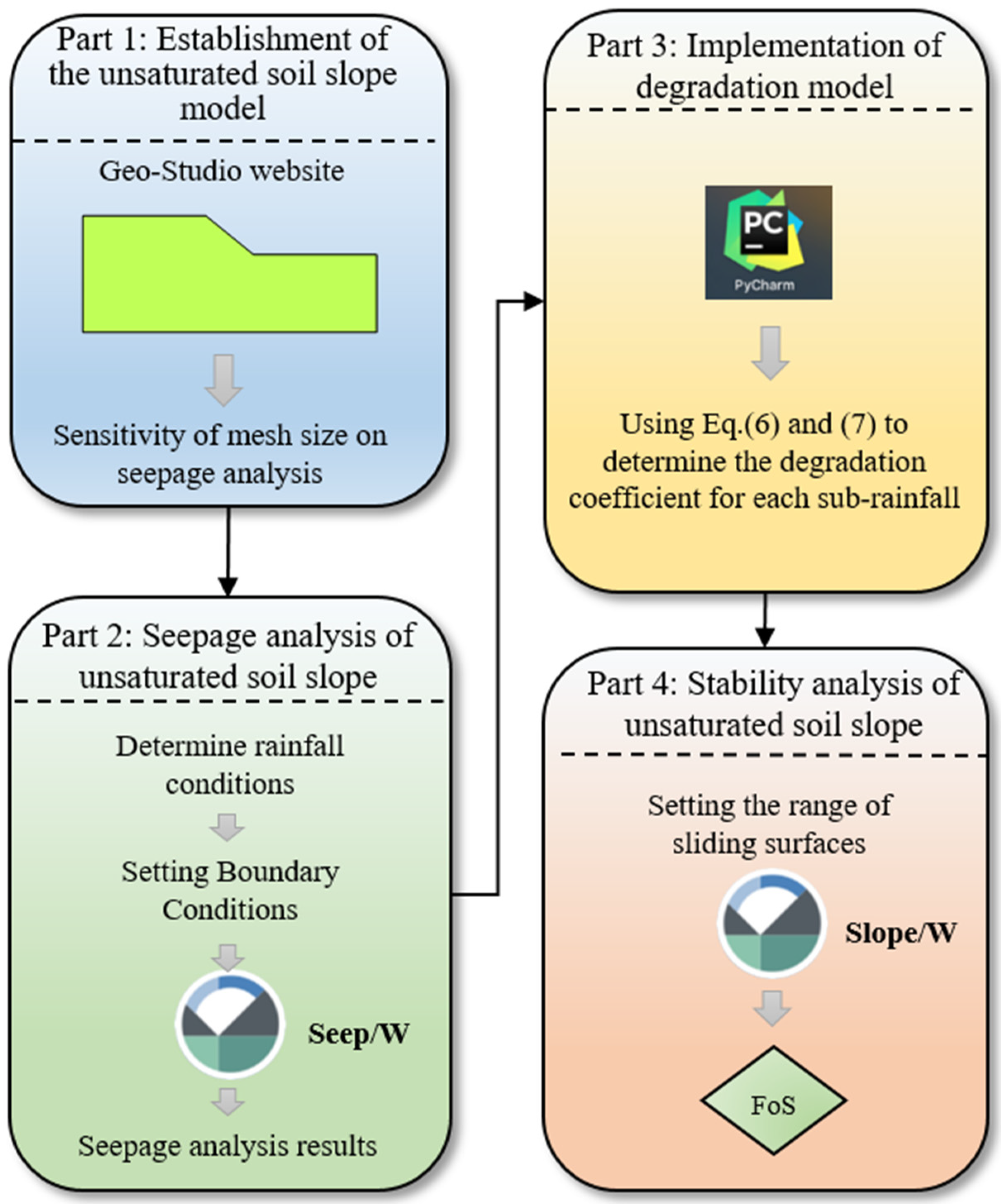
3. The Proposed Methodology

The flowchart of the proposed methodology is demonstrated in Figure 1. It can be seen that the proposed methodology consists of four parts: Part 1: establishment of the unsaturated soil slope model; Part 2: configuration of rainfall conditions; Part 3: implementation of degradation model; Part 4: stability analysis of unsaturated soil slope.
Referring to Figure 1, in Part 1, the unsaturated soil slope model is built using Geo-studio 2018 software package. To build the slope model, the slope geometry and the parameters of soil properties, such as unit weight, cohesion, internal friction angle, saturated permeability coefficient and SWCC related parameters, etc., should be determined in accordance with the site characterization report, and in situ or laboratory tests may be required if needed. Next, the sensitivity study of effect of mesh size on steady seepage analysis results is conducted to find a well-balanced mesh size from the perspectives of accuracy and efficiency. Finally, using the seepage analysis as parent analysis, the slope stability analysis is configured in Slope/w, where the circular slip surfaces and simplified Bishop method are selected. In Part 2, the intermittent rainfall conditions are configured, and then the seepage analysis is conducted via Seep/W module. In the second part, much attention is paid to applying rainfall boundary conditions and planning the calculation time steps. A rainfall infiltration boundary condition with surface run-off is imposed on the slope surface. A zero-flux boundary condition is applied on the bottom of slope. Finally, the seepage analyses are conducted following the designed calculation time steps regarding the intermittent rainfall. The obtained seepage results at all the designed time steps are stored for subsequent use in Slope/w. In Part 3, degradation model simulated using Equations (6) and (7) is implemented to obtain the degradation coefficient at all the designed time steps. Next, the degraded cohesion cD and internal friction angle φD are stored for the slope stability analysis. In Part 4, the degraded cohesion and internal friction angle are substituted for the original values to perform slope stability analysis. FoS values with degradation and without degradation are calculated using Slope/w and comparisons are made to provide insight into stability analysis of unsaturated soil slope.

4. Illustrative Examples

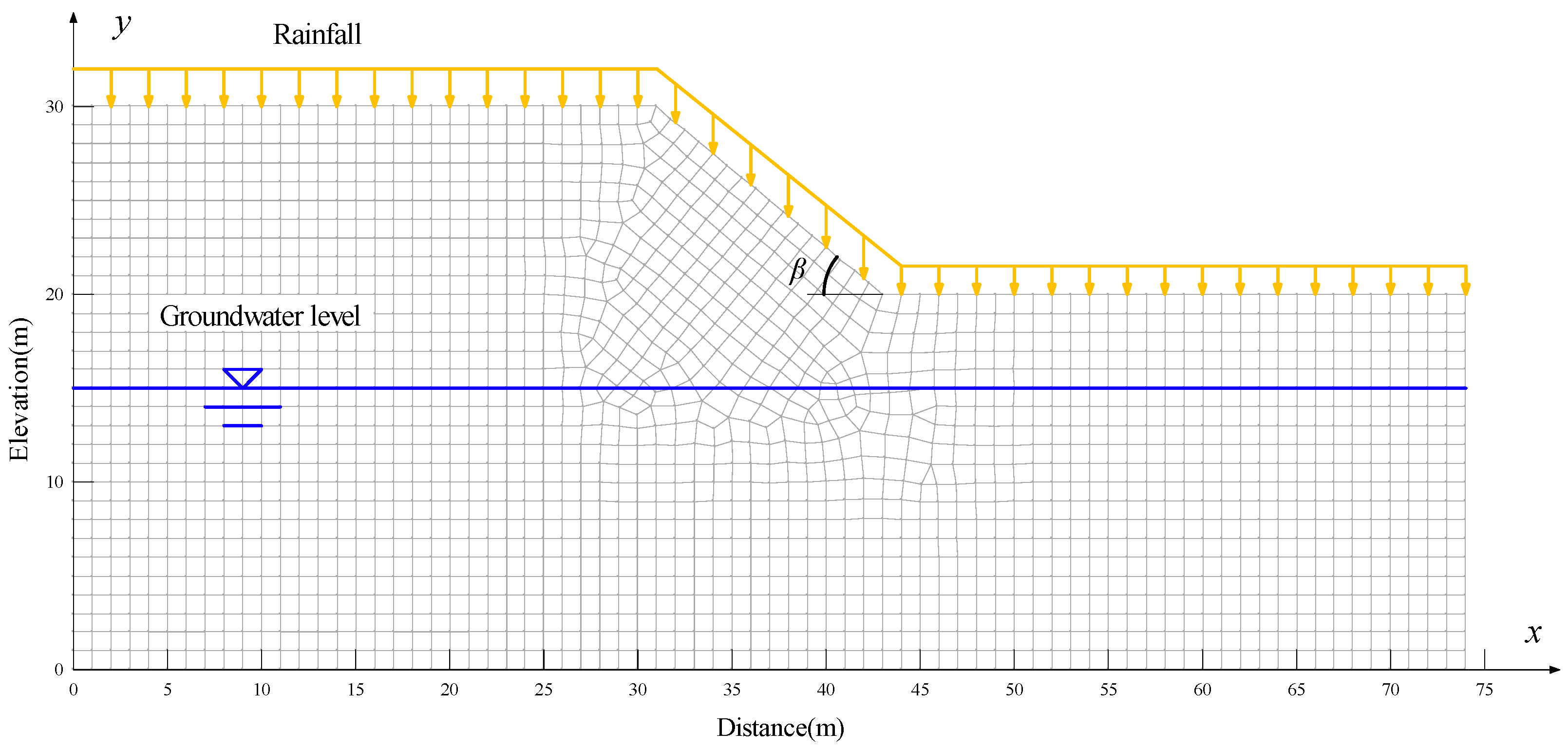
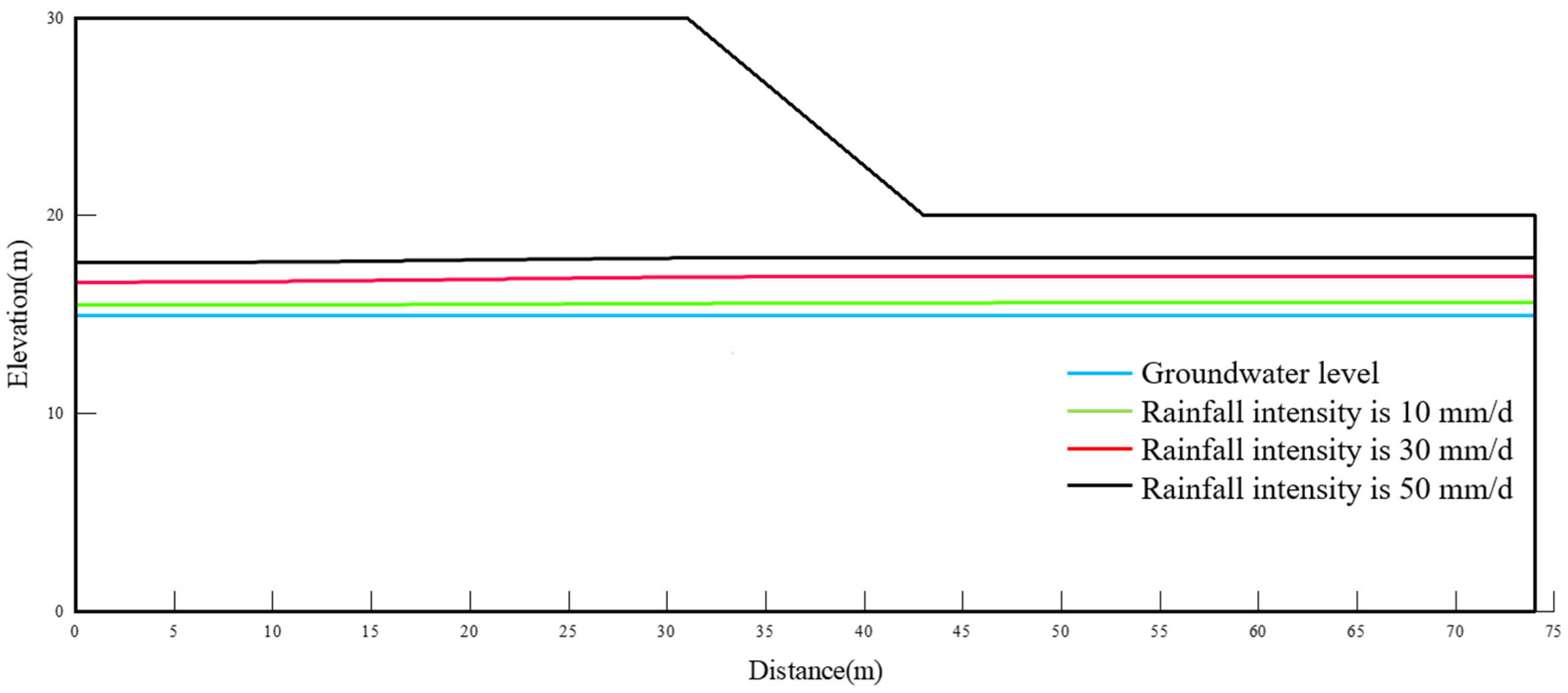
4.1. Establishment of Unsaturated Soil Slope Model

An illustrative example under rainfall conditions on the official website of Geo-studio (www.geoslope.com) is revisited in this study.
As shown in Figure 2, the homogeneous soil slope has a height of 10 m with an inclination angle (β) of 39.81°. Following the assumption in [5], the horizontal groundwater level is found 15 m below the top slope surface (i.e., at y = 15 m). It is worth noting that the horizontal groundwater level assumption may not be the case in practice, and the field monitoring records can be easily incorporated into the proposed study. The unit weight of soil denoted by γ is 20 kN/m3. The respective original cohesion c0 and friction angle φ0 are 2 kPa and 26°. The saturated permeability coefficient Ks is 1.0 × 10⁻⁶ m/s. Following the configurations at www.geoslope.com, the detailed parameters for the seepage and stability analysis are summarized in Table 1. The proper choice of hydraulic boundaries is important for seepage analysis. The left and right sides of the slope have a constant water head of 15 m to simulate an initial groundwater level. As signified by the hollow arrows in Figure 2, the rainfall infiltration condition with surface run-off is imposed on the slope surface. A zero-flux boundary condition is applied on the bottom and the left and right sides above the groundwater level. The results from the official website, www.geoslope.com, are regarded as the benchmark. A sensitivity study of the effect of mesh size on steady state seepage analysis was performed, and the consequent recommendation is a balanced mesh size = 0.5 m, leading to the combination of 7348 quadrilateral and triangular elements. Therefore, the mesh configuration of 7348 quadrilateral and triangular elements was adopted to conduct the transient seepage analysis with intermittent rainfall.
In the stability analysis using the Slope/w module in Geo-studio, the circular slip surface and simplified Bishop method are selected to calculate the FoS. The critical slip surface with the minimum FoS can be obtained by applying the entrance point on the slope surface between (25 m, 30 m) and (35 m, 26.7 m) and the exit point on the slope surface between (39 m, 23.3 m) and (50 m, 20 m). The default values for other related inputs in Slope/w are retained. Finally, the minimum FoS is used to evaluate the slope stability of unsaturated soils with intermittent rainfall.

4.2. Seepage and Stability Analysis of Slope with Intermittent Rainfall Without Considering Degradation of Soil Properties

Let Ri denote the intensity for the ith sub-rainfall, Tri denote the ith sub-rainfall duration, M denote the number of sub-rainfall, and Tei denote the rainfall intervals between the ith and i + 1th sub-rainfall within an intermittent rainfall. Based on the Rainfall Grade Standard published by the China Meteorological Administration (https://www.cma.gov.cn), the selected representative intensity values for moderate rain, heavy rain and torrential rain are 10, 30 and 50 mm/d, respectively. Table 2 lists the details of the designed intermittent rainfall. This section will investigate the impact of rainfall intensity, rainfall duration and rainfall intervals on the slope stability. As demonstrated in Table 2, a variety of intermittent rainfall scenarios can be designed by choosing one potential value from the corresponding list. Only part of the full total of combinations is considered in this section to study the influence of rainfall parameters.

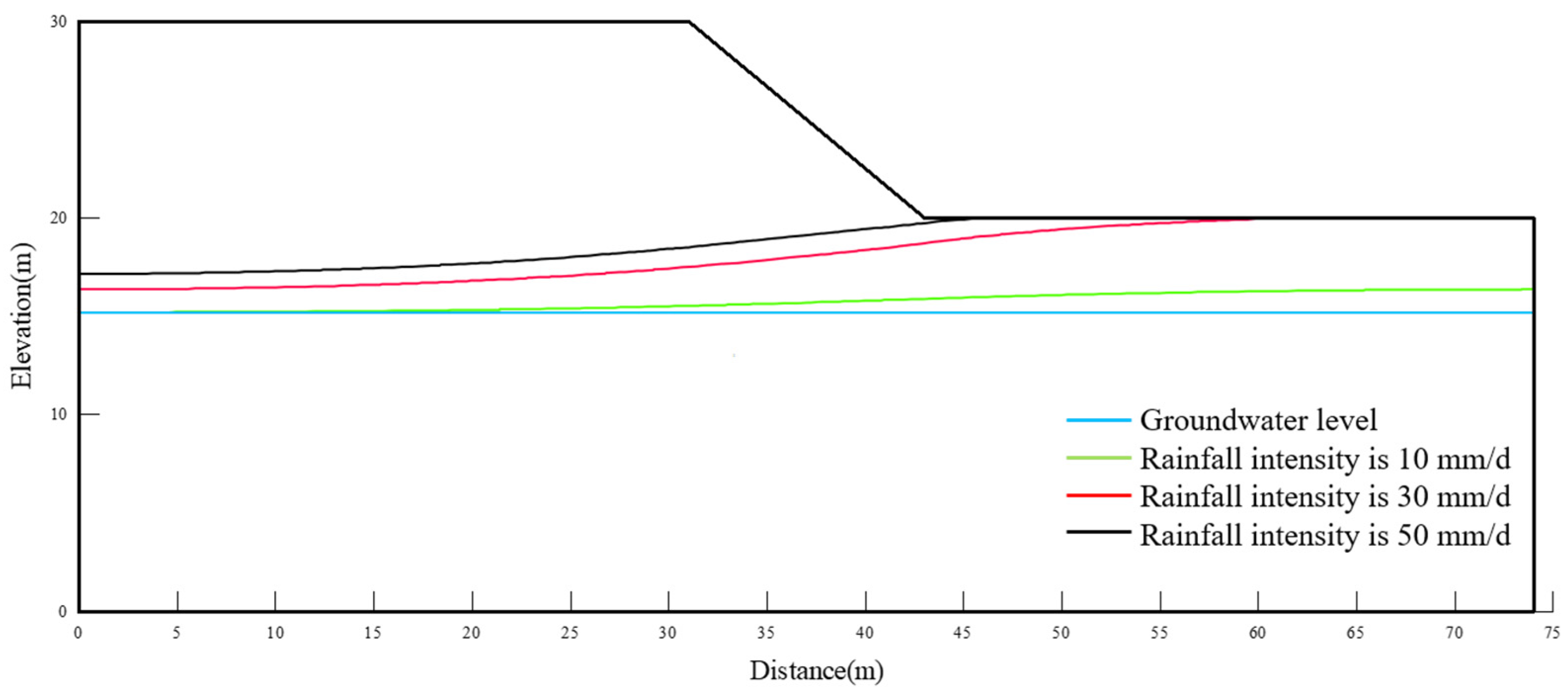
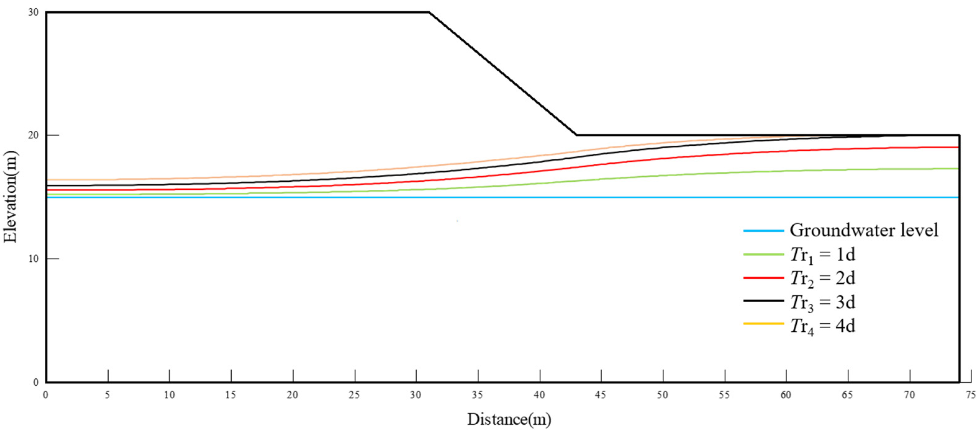
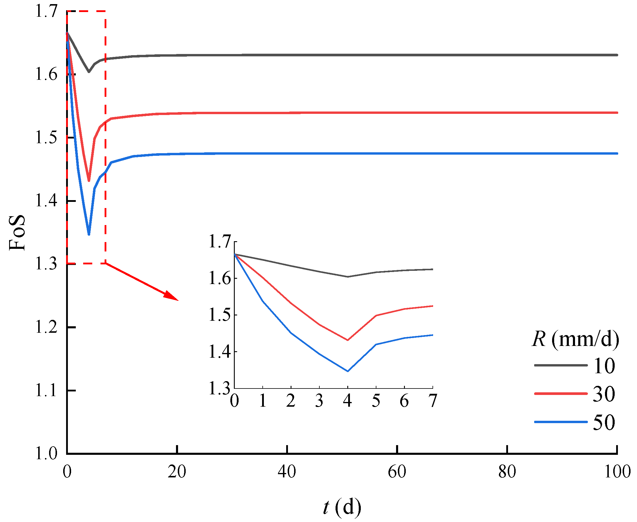
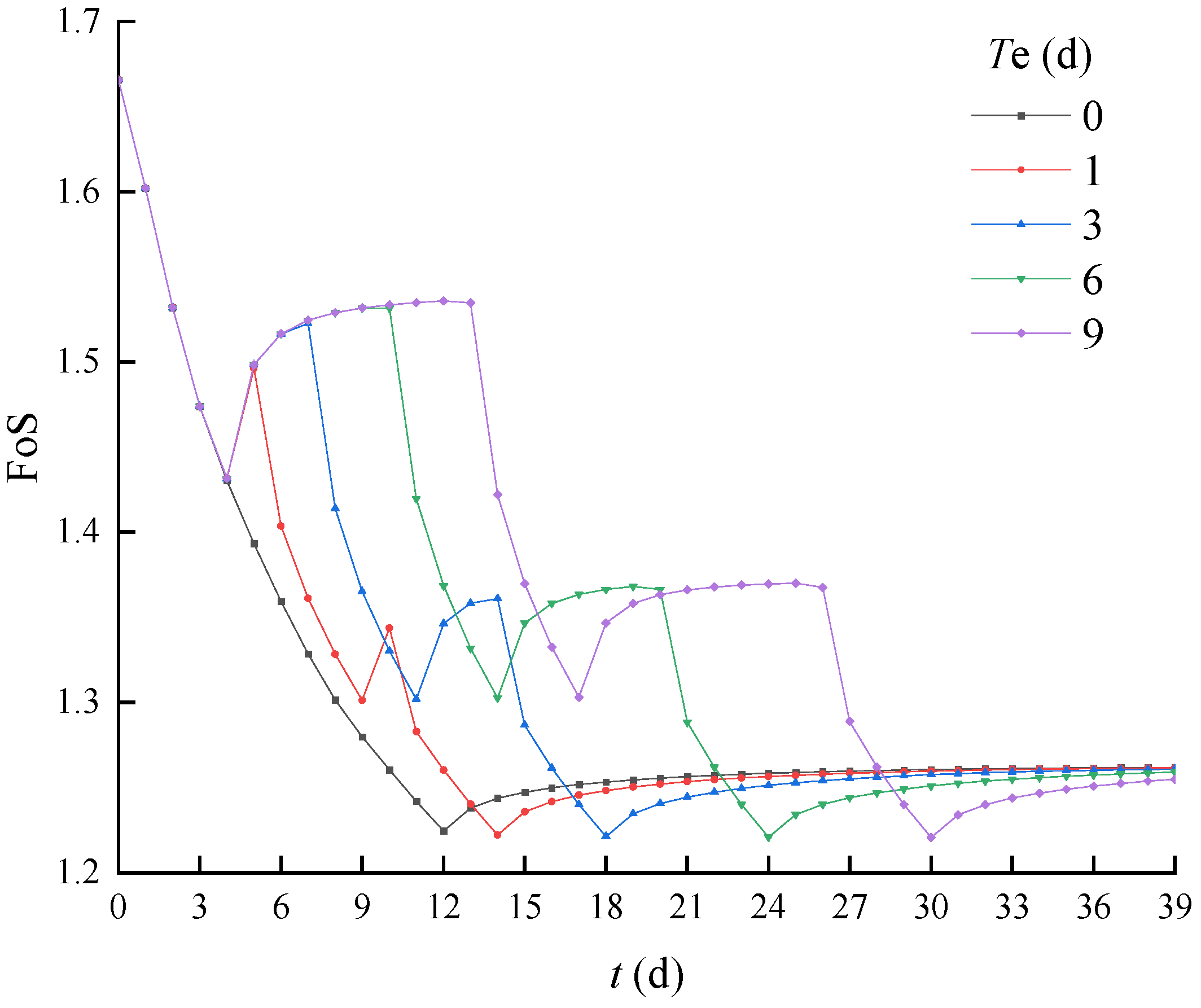
4.2.1. Impact of Rainfall Intensity and Rainfall Duration

Consider a special case of intermittent rainfall as an example, i.e., M = 1 and Tr1 = 4 d. R1 takes the values of 10, 30 and 50 mm/d, corresponding to moderate, heavy and torrential rainfall, respectively. The transient seepage analysis is conducted using the Seep/W module. The phreatic line connecting sequentially the points with zero pore water pressure is a straightforward indicator of slope stability, other things being equal. Usually, a higher phreatic line implies a lower slope stability, i.e., a smaller FoS. The respective phreatic lines corresponding to 10, 30 and 50 mm/d are depicted in Figure 3. The blue dashed line represents the initial phreatic line corresponding to the groundwater level, while the green, red and black dashed lines represent the phreatic line corresponding to R1 = 10, 30 and 50 mm/d, respectively. It can be seen that the originally horizontal phreatic line is ‘attracted’ to the slope surface, where the rainwater infiltrates into the slopes, facilitating the saturation of unsaturated soils and raising the phreatic line. It is expected that an intensity of 50 mm/d rainfall will have a larger flow velocity and a higher phreatic line than intensities of 30 mm/d and 10 mm/d. According to Figure 3, it can be observed that with the same Tr1, a larger R yields a higher phreatic line within the slope and a smaller resultant FoS.
Consider M = 1 and R1 = 30 mm/d (corresponding to heavy rainfall) as an example. Tr1 takes 1, 2, 3 and 4 d. The transient seepage analysis for each Tr1 is executed, and the phreatic line within the slope at t = Tr1 is located and plotted in Figure 4. As shown in Figure 4, the blue line represents the initial phreatic line corresponding to the groundwater level (y = 15 m), while the green, red, black and orange lines are the phreatic lines corresponding to t = Tr1 of 1, 2, 3 and 4 d, respectively. It is anticipated that for the same intensity of 30 mm/d rainfall, the phreatic line will tend to be closer to the slope surface at y = 20 m as the rainfall duration increases from 1 d to 4 d. As a result, when the rainfall intensity remains constant, the longer the rainfall duration, the higher the phreatic line within the slope. An elevated phreatic line increases the pore water pressure in the soil, which in turn reduces the effective stress and shear strength of the soil. As a result, the risk of slope failure (e.g., landslides or debris flows) may increase.
The seepage analysis results are further used for a slope stability analysis within the Slope/W module. Consider M = 1, Tr1 = 4 d and R1 = 10, 30 and 50 mm/d as an example. The calculation time step t ranges from 0 to 100 d. This means that 96 additional days are involved after the end of the rainfall. Figure 5 shows the variation of the FoS with t under R1 = 10, 30 and 50 mm/d. Take the first 7 days as an example. When R1 is 10 mm/d, the FoS values are 1.67, 1.65, 1.63, 1.61, 1.60, 1.61, 1.62 and 1.62, corresponding to t = 0, 1, 2, 3, 4, 5, 6 and 7 d. When R1 is 30 mm/d, the respective FoS values are 1.67, 1.60, 1.53, 1.47, 1.43, 1.49, 1.51 and 1.52 for t = 0, 1, 2, 3, 4, 5, 6 and 7 d. When R1 is 50 mm/d, the FoS values are 1.67, 1.53, 1.45, 1.39, 1.34, 1.41, 1.43 and 1.44 for t = 0, 1, 2, 3, 4, 5, 6 and 7 d. It can be noted from Figure 5 that for a given intensity of rainfall, the FoS drops to the minimum at the end of the rainfall and rises on the additional three days. This phenomenon is attributed to the fact that as the rainfall continues, the unsaturated soils become fully saturated and the phreatic line is elevated. The phreatic line reaches its highest location at the end of the rainfall, leading to the minimum FoS, and it begins to drop on the additional three days, owing to the sustained rainwater infiltration causing a rise in the FoS. Very similar variation trends have been observed for different intensities of rainfall, but the minimum FoS at the end of the rainfall differs. A higher intensity of rainfall leads to a smaller minimum FoS. It must be noted that once the rainfall ceases, the FoS of the slope slowly rises and finally converges to a constant value. For example, it converges to 1.62, 1.55 and 1.48 for R1 = 10, 30 and 50 mm/d, respectively. The explanation for this phenomenon is that since the rainfall stops, the rainwater continues infiltrating downwards until the maximum water storage is reached. In other words, the phreatic line tends to be unchanged once the rainwater no longer infiltrates downwards. Consequently, it can be inferred that without considering the impact of water evaporation, the final phreatic line within the slope under different rainfall intensities will display distinct disparities even after a sufficiently large number of additional time steps t (96 d in this study).
To further illustrate the increases in FoS within the additional three days after the end of the rainfall, the locations of the phreatic lines for R1 = 10, 30 and 50 mm/d at t = 7 d are plotted in Figure 6. As shown in Figure 6, the blue dashed line represents the initial phreatic line, while the green, red and black lines denote the phreatic lines for R1 = 10, 30 and 50 mm/d, respectively, at t = 7d. By comparing the phreatic lines in Figure 3 and Figure 6, it becomes evident that the curved phreatic lines in Figure 3 are all reshaped as horizontal lines. This indicates that after the end of the rainfall, the rainwater continues to infiltrate downwards, making the saturated soils close to the slope surface unsaturated again. This transformation of the soils from saturated to unsaturated yields a rise in FoS, which can be observed in Figure 5. In addition, a higher intensity of rainfall results in a higher phreatic line at t = 7 d and, hence, the FoS with the higher intensity of rainfall is smaller than that with the lower intensity of rainfall.

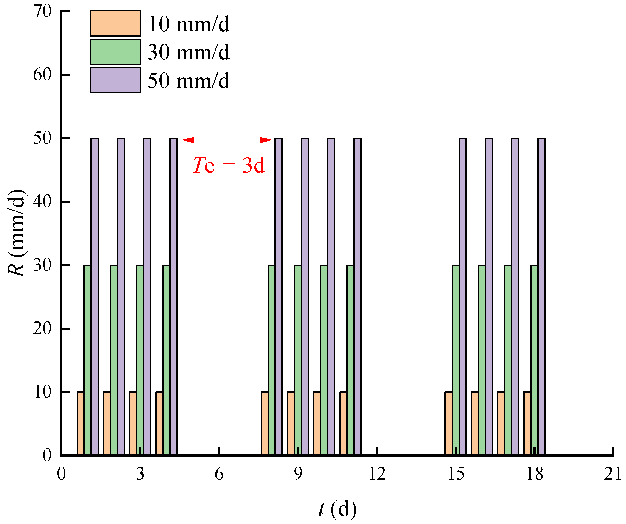
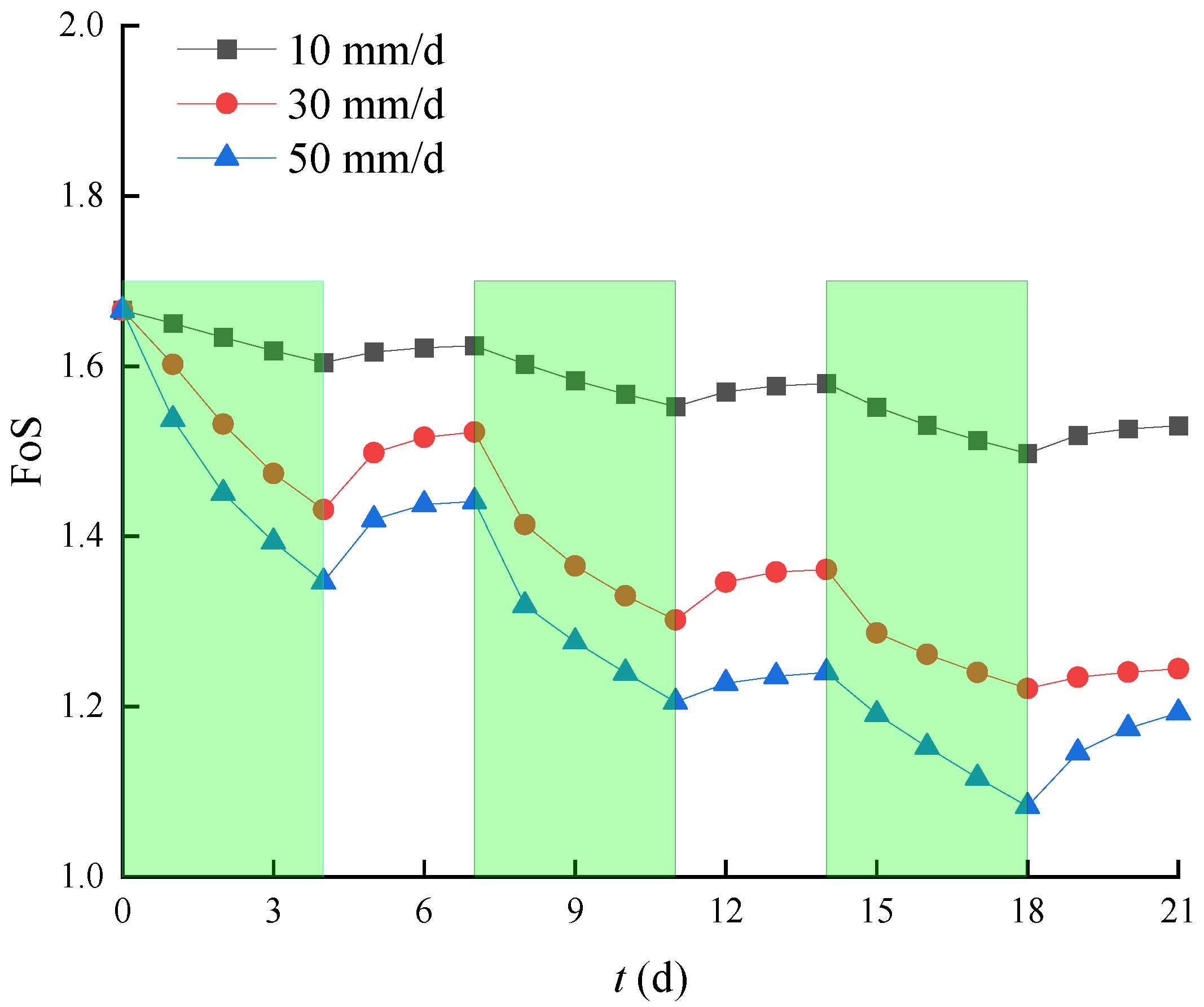
4.2.2. Impact of M and Rainfall Intervals

Figure 7 illustrates three scenarios of intermittent rainfall with M = 3, Tr1 = Tr2 = Tr3 = 4 d, Te1 = Te2 = 3 d and R1 = R2 = R3 = 10, 30 and 50 mm/d. The calculation time step t ranges from 0 to 21 d. For each rainfall intensity, the transient seepage analysis was conducted using Seep/w, and the obtained results were used in Slope/w to calculate the FoS.
Figure 8 plots the variation of the FoS with time step t for R1 = R2 = R3 = 10, 30 and 50 mm/d. The green part of the graph shows the rainfall holding time. Taking R1 = R2 = R3 = 50 mm/d (representative of torrential rainfall) as an example, the respective FoS values are 1.67, 1.53, 1.45, 1.39, 1.34, 1.41, 1.43, 1.44, 1.31, 1.27, 1.23, 1.20, 1.22, 1.23, 1.24, 1.19, 1.15, 1.11, 1.08, 1.14, 1.17 and 1.19. It is demonstrated that the variation curve of the FoS with time step t is divided into three separate sub-curves, each of which is similar to those in Figure 5. The minimum bold FoS 1.34, 1.20 and 1.08, are found at t = 4, 11 and 18 d, corresponding to the end of the first sub-rainfall, second sub-rainfall and third sub-rainfall, respectively. As explained in Section 4.2.1, the FoS after one sub-rainfall is unable to restore the original one (before the sub-rainfall, i.e., at t = 0, 7 and 14 d). It is anticipated that as M increases, the slope stability will deteriorate continuously until failure. As a result, the reinforcement works should be executed before the FoS is decreased to a value necessitating the early warning. Referring to the technical code for building slope engineering (GB 50330-2013) [43], the illustrative slope shown in Figure 2 is classified into Grade 3 and the allowable FoS is 1.25. From this perspective, after the end of the second rainfall, managers should implement reinforcement or drainage works to enhance the slope stability, because the FoS 1.20 is smaller than the recommended value of 1.25. Similarly, the minimum FoS values found at t = 4, 11 and 18 d are 1.60, 1.55 and 1.49 for an intensity of rainfall = 10 mm/d (representative of moderate rainfall), and they are 1.43, 1.30 and 1.22 for R1 = R2 = R3 = 30 mm/d (representative of heavy rainfall). It is found that for heavy rainfall, the reinforcement or drainage works should be executed after the end of the third sub-rainfall, and no reinforcement or drainage works is required for moderate rainfall under M = 3.
Figure 9 plots the variations of the FoS under different rainfall intervals. Consider M = 3, Tr1 = Tr2 = Tr3 = 4 d, R1 = R2 = R3 = 30 mm/d and Te1 = Te2 = 0, 1, 3, 6 and 9 d as an example. When Te1 = Te2 = 0 d, the intermittent rainfall turns out to be a special case, continuous rainfall. The initial FoS of the slope is 1.67, it drops dramatically to the minimum value of 1.22 at the end of the rainfall (t = 12 d), and then it rises slightly, and finally converges to a constant value, as described in Figure 5. In the case of Te1 = Te2 = Te3 = 1 d, the minimum FoS values at the end of three sub-rainfalls (t = 4, 9 and 14 d) are 1.43, 1.30 and 1.22. In the case of Te1 = Te2 = Te3 = 3 d, the minimum FoS values at the end of three sub-rainfalls (t = 4, 11 and 18 d) are 1.43, 1.30 and 1.22. As for Te1 = Te2 = Te3 = 6 d, the minimum FoS values at the end of three sub-rainfalls (t = 4, 14 and 24 d) are 1.43, 1.30 and 1.22. When the rainfall intervals are increased to 9 d, the minimum FoS values at the end of three sub-rainfalls (t = 4, 17 and 30 d) are 1.43, 1.30 and 1.22. It is observed that the minimum Fos values at the end of the first sub-rainfall, i.e., at t = 4 d for Te1 = Te2 = 0, 1, 3, 6 and 9 d, are all equal to 1.43. Furthermore, the minimum Fos values at the end of the second sub-rainfall, i.e., at t = 8, 9, 11, 14 and 17 d for Te1 = Te2 = 0, 1, 3, 6 and 9 d arrive at an identical value of 1.30. Finally, the minimum Fos values at the end of the third sub-rainfall i.e., at t = 12, 14, 18, 24 and 30 d for Te1 = Te2 = 0, 1, 3, 6 and 9 d reach an identical value of 1.22, demonstrating that the Te does not affect the minimum FoS caused by each sub-rainfall. It can be expected that the final converged FoS values after a sufficiently large number of additional days at the end of the third rainfall will be identical, in accordance with the observations in Figure 5.

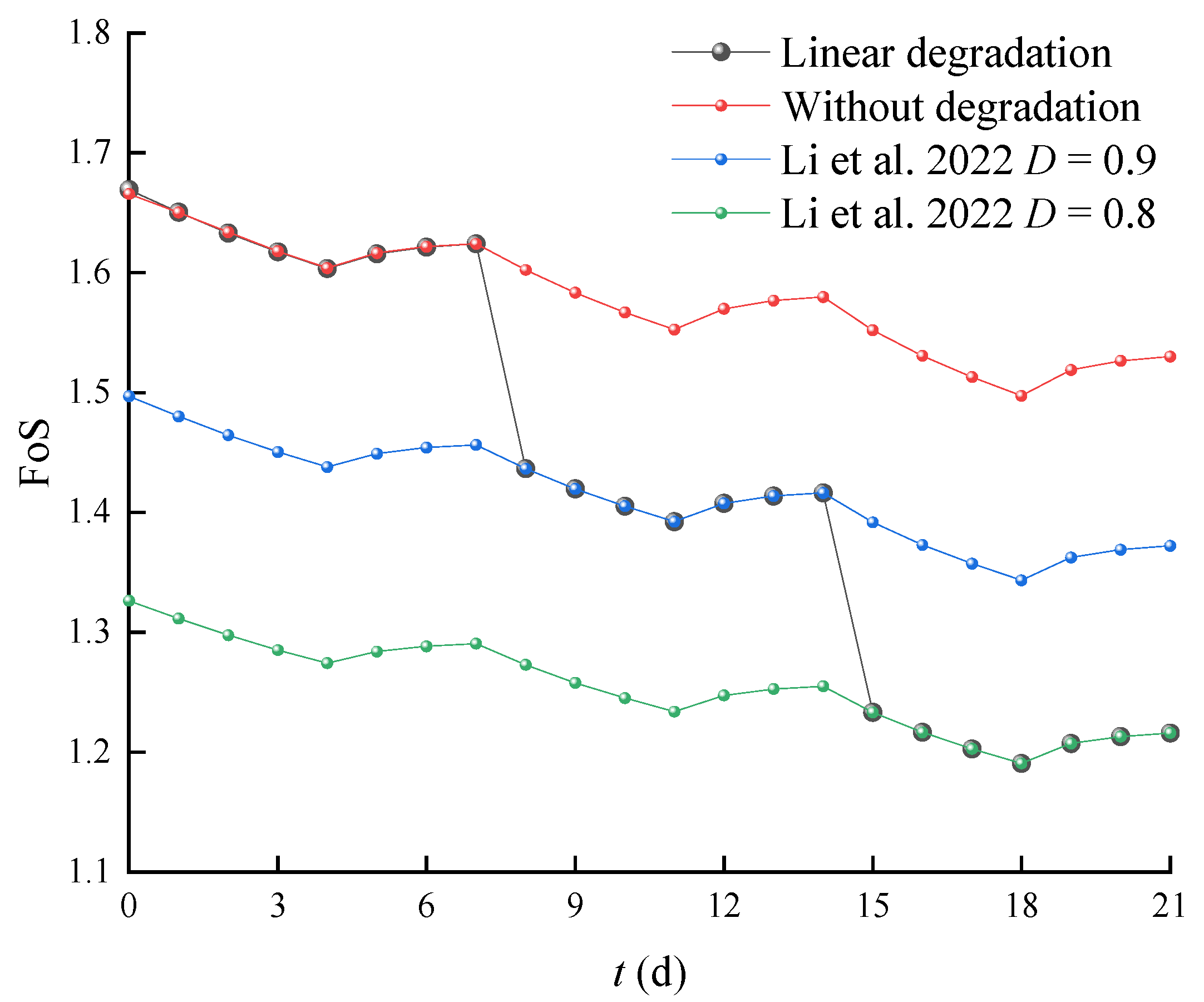
4.3. Slope Stability Analysis with Intermittent Rainfall Considering Linear Degradation of Soil Properties

The simplified linear degradation model described in Equation (6) is illustrated in this section. It must be noted that the crucial parameters for the simplified degradation model are b, E and Dmin. The determination of these three parameters should be based on laboratory tests. In the current study, b = 1, E = 6 and Dmin = 0.5 are tentatively specified, simply to demonstrate the necessity of considering the degradation of soil properties in the stability analysis of unsaturated soil slopes. Referring to Equation (6), k = 0.1 is determined.
Consider M = 3, Tr1 = Tr2 = Tr3 = 4 d, R1 = R2 = R3 = 10 mm/d and Te1 = Te2 = 3 d as an example. The seepage analysis presented in Section 4.2.2 was reused for a further stability analysis, since the degradation of hydraulic parameters such as the permeability coefficient is not considered in this study. Referring to Equation (6), the degradation coefficient of soil properties such as cohesion and friction angle is determined to be 1.0, 0.9 and 0.8 for the first, second and third sub-rainfalls. The original cohesion and friction angle are multiplied by the degradation coefficient to determine the degraded cohesion and internal friction angle, which are substituted for the original cohesion and internal friction angle in the stability analysis in Slope/w. Figure 10 plots the variations of the FoS with time step t for the scenarios of considering degradation and without considering degradation.
It can be noted from Figure 10 that as t ranges from 0 to 21 d, the corresponding FoS values are 1.67, 1.65, 1.63, 1.61, 1.60, 1.61, 1.62, 1.62, 1.60, 1.58, 1.56, 1.55, 1.56, 1.57, 1.58, 1.55, 1.53, 1.51, 1.49, 1.51, 1.52 and 1.53 without considering the degradation of the soil properties. The corresponding FoS values of the slope are 1.67, 1.65, 1.63, 1.61, 1.60, 1.61, 1.62, 1.62, 1.43, 1.41, 1.40, 1.39, 1.40, 1.41, 1.41, 1.23, 1.21, 1.20, 1.19, 1.20, 1.21 and 1.22 when the degradation of the soil properties is considered using the simplified linear degradation model. This comparison indicates that the second and third minimum FoS values of 1.55 and 1.49 change to 1.39 and 1.19 after the degradation of the soil properties is considered. Referring to the technical code for building slope engineering (GB 50330-2013) [43], the illustrative slope shown in Figure 2 is classified into Grade 3, and the allowable FoS is 1.25. When the degradation of the soil properties is considered, reinforcement and drainage works should be implemented, since the third minimum FoS 1.19 is smaller than the allowable FoS, 1.25, although they are not necessary, as mentioned in the previous section, when the degradation of the soil properties is omitted. Since the degradation of soil properties is inevitable, its influence on the stability of unsaturated soil slopes should be properly considered. The simplified linear degradation model is a promising attempt.
The results calculated by the constant and instantaneous degradation model proposed in [29] are included in Figure 10 for comparison. In the constant and instantaneous degradation model in [29], a constant degradation coefficient is applied. D = 0.9 and 0.8 are assumed for the constant and instantaneous degradation model. As depicted in Figure 10 using blue circles, the minimum FoS values at the end of each sub-rainfall (at t = 4, 11 and 18 d) are 1.44, 1.39 and 1.34, respectively, for D = 0.9. In the case of D = 0.8, the respective minimum FoS values at the end of each sub-rainfall (at t = 4, 11 and 18 d) are 1.27, 1.23 and 1.19. These comparisons demonstrate that the constant and instantaneous degradation model cannot model the progressive deterioration in FoS owing to the degradation in soil properties due to the rainfall infiltrations. At D = 0.9, the constant and instantaneous degradation model tends to underestimate the FoS for the first sub-rainfall, while it tends to overestimate the FoS for the third sub-rainfall. In the case of D = 0.8, it leads to the underestimation of the FoS for the first and second sub-rainfalls. As a result, the simplified linear degradation model is warranted.

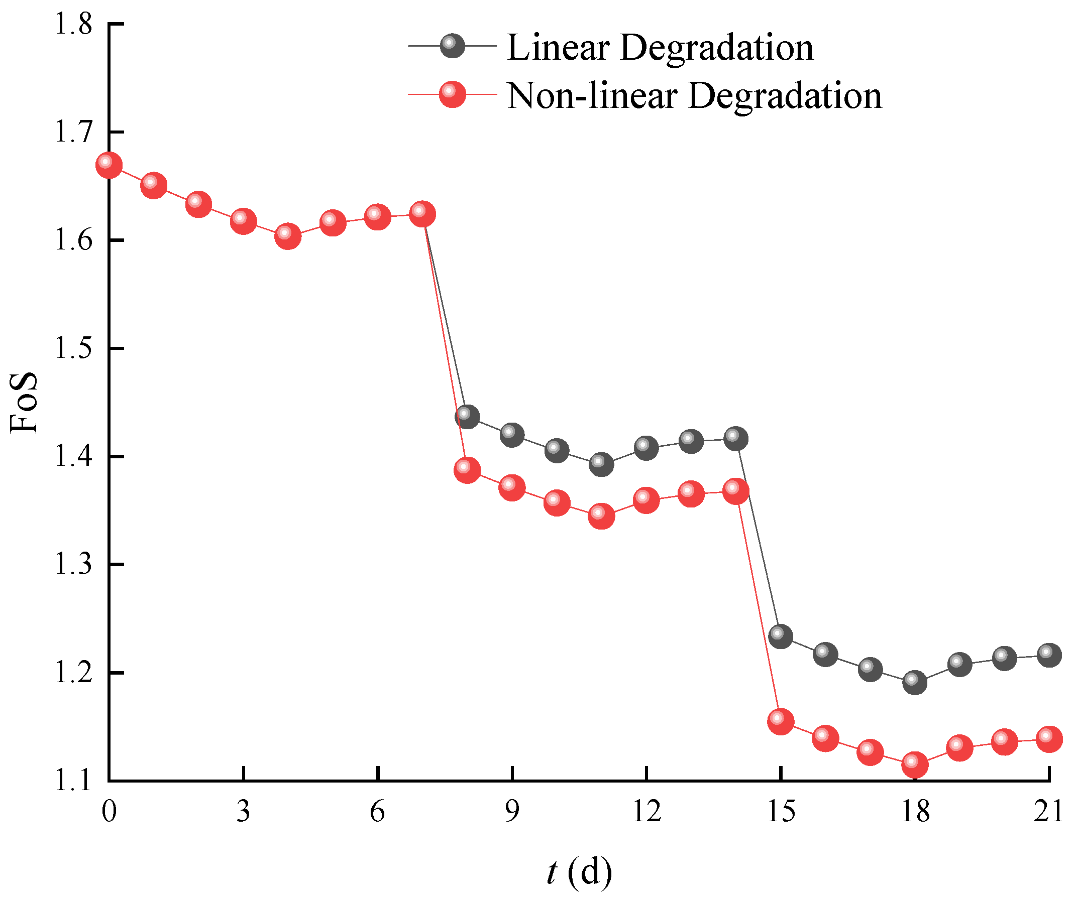
4.4. Slope Stability Analysis with Intermittent Rainfall Considering Non-Linear Degradation of Soil Properties

In Section 4.3, the results from the linear degradation model are discussed, whereas in this section, the results from the nonlinear degradation model are described. To ensure consistent comparison, the identical independent parameters are adopted, i.e., b = 1, E = 6 and Dmin = 0.5. Referring to Equation (7), the dependent ξ is determined to be 0.1386.
Consider M = 3, Tr1 = Tr2 = Tr3 = 4 d, R1 = R2 = R3 = 10 mm/d and Te1 = Te2 = 3 d as an example. The seepage analysis presented in Section 4.2.2 is reused for further stability analysis, since the degradation of hydraulic parameters such as the permeability coefficient is not considered in this study. Referring to Equation (7), the degradation coefficient of soil properties such as cohesion and friction angle is determined to be 1.0, 0.87 and 0.75 for the first, second and third sub-rainfalls. The original cohesion and friction angle are multiplied by the degradation coefficient to determine the degraded cohesion and internal friction angle, which are substituted for the original cohesion and internal friction angle in the stability analysis in Slope/w. Figure 11 compares the variations of the FoS with time step t between the linear and nonlinear degradation models.
Figure 11 shows that when t ranges from 0 to 21 d, the corresponding FoS values for the slope are 1.67, 1.65, 1.63, 1.61, 1.60, 1.61, 1.62, 1.62, 1.39, 1.37, 1.36, 1.34, 1.36, 1.37, 1.37, 1.15, 1.14, 1.13, 1.11, 1.13, 1.14 and 1.14, respectively, when the nonlinear degradation model is adopted. It is observed that the second and third minimum FoS values of 1.39 and 1.19 with the linear degradation model turn out to be 1.34 and 1.11 with the nonlinear degradation model. It is revealed that the nonlinear degradation model yields a smaller FoS (corresponding to a more conservative decision) than the linear degradation model.

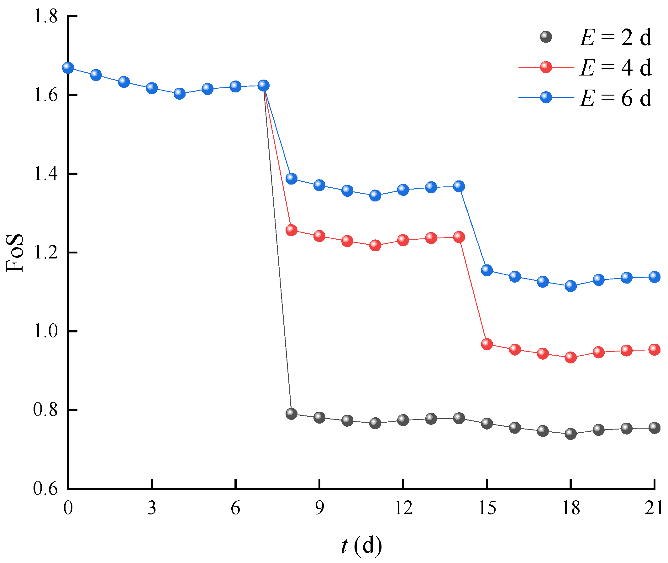
4.5. Sensitivity Analysis of Parameters in Nonlinear Degradation Model

The nonlinear degradation coefficient is influenced by the characteristics of rainfall, soil properties and slope geometry, which are crucial factors in slope stability analysis [44,45]. Sensitivity analysis is a crucial method for evaluating the degree to which model output results respond to changes in input parameters. Based on the two key input parameters determined in the previous sections, E and Dmin (the latter of which shows a significant correlation with rainfall intensity), this section will systematically assess the sensitivity of these parameters to the FoS using the nonlinear degradation model constructed in Section 4.4, emphasizing the patterns of the impact of E and Dmin on the FoS.

4.5.1. Impact of Parameter E

Although repeated water infiltration leads to a progressive degradation of the cohesion and internal friction angle, this degradation process exhibits a significant threshold effect, that is, when the number of infiltration cycles reaches a critical value E, the soil strength parameters tend to stabilize and form a new mechanical equilibrium state. To systematically reveal the control mechanism of this critical threshold in relation to slope stability, a parametric study is conducted using the control variable method, relying on the conditions listed in Table 3.
Consider M = 3, Tr1 = Tr2 = Tr3 = 4 d, R1 = R2 = R3 = 10 mm/d and Te1 = Te2 = 3 d as an example. Referring to the scenarios presented in Table 3, when E = 2 d and Dmin = 0.5, the value of ξ is determined to be 0.6931 using Equation (7). The degradation coefficient of soil properties such as cohesion and friction angle is determined to be 1.0, 0.5 and 0.5 for the first, second and third sub-rainfalls. When E = 4 d and Dmin = 0.5, the value of ξ is 0.2310. The degradation coefficient of the cohesion and friction angle is determined to be 1.0, 0.79 and 0.63 for the first, second and third sub-rainfalls. When E = 6 d and Dmin = 0.5, the value of ξ is 0.1386. The degradation coefficient of the cohesion and friction angle is determined to be 1.0, 0.87 and 0.75 for the first, second and third sub-rainfalls. The variation of the calculated FoS with t at different values of E is shown in Figure 12.
Figure 12 reveals that when E is equal to 2 d, the second and third minimum FoS values are 0.77 and 0.74, respectively. When E is 4 d, the corresponding minimum FoS values are 1.22 and 0.93. When E is 6 d, the second and third minimum FoS values are 1.34 and 1.11, respectively. It can be observed that the smaller the value of E, the lower the FoS.

4.5.2. Impact of Parameter Dmin

Since the Dmin is intuitively dependent on rainfall intensity, three scenarios for Dmin are designed in Table 4. It is noted that a larger rainfall intensity corresponds to a lower Dmin. The intrinsic interaction mechanism between rainfall intensity and Dmin needs to be elucidated through a comprehensive hydro-mechanical coupling model. To systematically reveal the impact of Dmin on FoS, a parametric study of Dmin is performed using the control variable method, depending on the scenarios listed in Table 4.
Consider M = 3, Tr1 = Tr2 = Tr3 = 4 d and Te1 = Te2 = 3 d as an example. Referring to the scenarios presented in Table 4, when E = 6 d, R = 10 mm/d and Dmin = 0.5, the value of ξ is determined to be 0.1386. The degradation coefficient of the cohesion and friction angle is determined to be 1.0, 0.87 and 0.75 for the first, second and third sub-rainfalls. When E = 6 d, R =20 mm/d and Dmin = 0.45, the value of ξ is 0.1597. The degradation coefficient of the cohesion and friction angle is determined to be 1.0, 0.85 and 0.73 for the first, second and third sub-rainfalls. When E = 6 d, R = 30 mm/d and Dmin = 0.4, the value of ξ is 0.1833. The degradation coefficient of the cohesion and friction angle is determined to be 1.0, 0.83 and 0.69 for the first, second and third sub-rainfalls. The variation of the calculated FoS with t at different values of Dmin is shown in Figure 13.
Figure 13 demonstrates that when Dmin = 0.5 and R = 10 mm/d, the second and third minimum FoS are 1.34 and 1.11, respectively. When Dmin = 0.45 and R = 20 mm/d, the corresponding minimum FoS values are 1.18 and 0.94. When Dmin = 0.4 and R = 30 mm/d, the second and third minimum FoS are 1.08 and 0.84, respectively. It can be observed that the smaller the value of Dmin, the lower the FoS.

5. Discussion

Intermittent rainfall is well acknowledged, and its influence on the stability of unsaturated soil slopes has attracted worldwide attention. In the introduction section, the literature review warranted the consideration of the degradation of soil properties in slope stability analysis. Previous research [29] developed a constant and instantaneous degradation model and underscored the significance of incorporating the degradation in the cohesion and internal friction angle within rainfall. The current study attempts to introduce simplified linear and nonlinear degradation models, whose crucial parameters can be determined based on laboratory tests. One limitation of this study is that the degradation of hydraulic parameters such as the permeability coefficient is not considered. The other limitation of this study is that it assumes identical degradation of the cohesion and internal friction angle, which may not be the case in practical engineering. Furthermore, the rainfall intensity is assumed to be identical for all the sub-rainfall durations, and the rainfall intervals are also identical between adjacent rainfalls. Last, but not least, the influence of rainfall intensity on the degradation of soil properties was missed due to the lack of experimental data. Despite the aforementioned limitations, the current study endeavors to investigate the influence of rainfall intervals and the number of rainfalls within intermittent rainfall on the FoS of unsaturated soil slopes. It is noted that before the simplified degradation model can be used for stability analysis, the original cohesion and internal friction angle should be re-determined using in situ or laboratory tests because the previous rainfalls may deteriorate the soil properties. In the future, attention may be paid to the development of a practical degradation model based on laboratory direct shear tests. In addition to the numerical models, the early warning system acts as an effective tool for predicting slope stability and making decisions on reinforcement works. It is worth noting that the combination of the proposed degradation model with an early warning system would contribute to the slope stability evaluation under rainfall conditions. For example, the field monitoring of rainfall records can be utilized in the proposed degradation models, and the degraded FoS facilitates the decision making in turn. Finally, it is noted that although short-term slope stability is focused on in the present study, in which a maximum 21 days is considered, the long-term slope stability can be properly assessed using the current method while carefully updating the crucial parameters of the degradation models. For example, the micro-structure of soils tends to be changed within no-rainfall periods, and the progressive failure behavior of soils may be incorporated into the long-term slope stability.

6. Conclusions

Rainfall-induced landslides are well recognized in tropical areas. To properly assess the stability of unsaturated soil slopes in order to facilitate decision making as to the early warning treatment, a simplified linear degradation model was developed. The sensitivity studies on a number of sub-rainfalls and rainfall intervals were conducted against an illustrative slope example extracted from the official Geo-studio website. The results from the simplified linear degradation model were compared with those from the previous constant and instantaneous degradation model. The comparisons manifest the following:
(1)
The number of sub-rainfalls within one intermittent rainfall exerts a significant influence on the FoS values of unsaturated soil slopes, whereas the influence of rainfall intervals on the minimum FoS at the end of each sub-rainfalls is negligible.
(2)
The simplified linear degradation model can simulate the progressive deterioration in the FoS due to the degradation of soil properties induced by rainfall infiltration, whilst the constant and instantaneous degradation model tends to overestimate or underestimate the FoS as compared to the linear degradation model.
(3)
Even for moderate rainfall, reinforcement and drainage works should be implemented after considering the degradation of the soil properties induced by intermittent rainfall infiltration, although they are unnecessary when the degradation of the soil properties is omitted.
It is noted that the incorporation of degradation models in slope stability analysis helps to make decisions on reinforcement and drainage works. In addition, employing Microbial Induced Carbonate Precipitation (MICP) technology to reduce the surface soil permeability and planting vegetation to enhance surface runoff are two promising measures for landslide risk mitigation.

Author Contributions

Conceptualization, L.L.; Original draft, M.W. All authors have read and agreed to the published version of the manuscript.

Funding

This research received no external funding.

Data Availability Statement

Most of the data generated during this study are included in the article. For other datasets, please contact the corresponding author at liliang@qut.edu.cn.

Acknowledgments

Thanks to all the anonymous reviewers for their valuable comments, which improved quality of our paper.

Conflicts of Interest

The authors declare no conflicts of interest.

References

  1. Guzzetti, F.; Mondini, A.C.; Cardinali, M.; Fiorucci, F.; Santangelo, M.; Chang, K.-T. Landslide inventory maps: New tools for an old problem. Earth-Sci. Rev. 2012, 112, 42–66. [Google Scholar] [CrossRef]
  2. Tang, G.; Huang, J.; Sheng, D.; Sloan, S.W. Stability analysis of unsaturated soil slopes under random rainfall patterns. Eng. Geol. 2018, 245, 322–332. [Google Scholar] [CrossRef]
  3. Wang, B.; Vardon, P.; Hicks, M. Rainfall-induced slope collapse with coupled material point method. Eng. Geol. 2018, 239, 1–12. [Google Scholar] [CrossRef]
  4. Song, X.; Tan, Y. Experimental study on failure of temporary earthen slope triggered by intense rainfall. Eng. Fail. Anal. 2020, 116, 104718. [Google Scholar] [CrossRef]
  5. Liu, X.; Wang, Y.; Leung, A.K. Numerical investigation of rainfall intensity and duration control of rainfall-induced landslide at a specific slope using slope case histories and actual rainfall records. Bull. Eng. Geol. Environ. 2023, 82, 1–20. [Google Scholar] [CrossRef]
  6. Zong, J.; Zhang, C.; Liu, L.; Liu, L. Modeling Rainfall Impact on Slope Stability: Computational Insights into Displacement and Stress Dynamics. Water 2024, 16, 554. [Google Scholar] [CrossRef]
  7. Zhuang, Y.; Hu, X.; He, W.; Shen, D.; Zhu, Y. Stability Analysis of a Rocky Slope with a Weak Interbedded Layer under Rainfall Infiltration Conditions. Water 2024, 16, 604. [Google Scholar] [CrossRef]
  8. Kluger, M.O.; Jorat, M.E.; Moon, V.G.; Kreiter, S.; de Lange, W.P.; Mörz, T.; Robertson, T.; Lowe, D.J. Rainfall threshold for initiating effective stress decrease and failure in weathered tephra slopes. Landslides 2020, 17, 267–281. [Google Scholar] [CrossRef]
  9. Ng, J.N.; Taib, A.M.; Razali, I.H.; Rahman, N.A.; Mohtar, W.H.M.W.; Karim, O.A.; Desa, S.M.; Awang, S.; Mohd, M.S.F. The Effect of Extreme Rainfall Events on Riverbank Slope Behaviour. Front. Environ. Sci. 2022, 10, 859427. [Google Scholar] [CrossRef]
  10. Li, L.; Ju, N.; He, C.; Li, C.; Sheng, D. A computationally efficient system for assessing near-real-time instability of regional unsaturated soil slopes under rainfall. Landslides 2019, 17, 893–911. [Google Scholar] [CrossRef]
  11. Zhang, J.; Li, J.; Lin, H. Models and influencing factors of the delay phenomenon for rainfall on slope stability. Eur. J. Environ. Civ. Eng. 2018, 22, 122–136. [Google Scholar] [CrossRef]
  12. Yang, Y.; Cai, R.; Zhang, G.; Su, S.; Liu, W. Evaluating and analyzing the stability of loess slope using intermittent rainfall and various rainfall patterns. Arab. J. Geosci. 2022, 15, 218. [Google Scholar] [CrossRef]
  13. Li, Z.; Zhao, J.; Lv, S.; Liu, L.; Zhang, C. Investigations of the Effect of Artificial Rainfall on the Pore Water Pressure and Slope Surface Displacement of Loess Slopes. Int. J. Géoméch. 2024, 24, 04024064. [Google Scholar] [CrossRef]
  14. Cai, J.-S.; Yeh, T.-C.J.; Yan, E.-C.; Tang, R.-X.; Hao, Y.-H.; Huang, S.-Y.; Wen, J.-C. Importance of variability in initial soil moisture and rainfalls on slope stability. J. Hydrol. 2019, 571, 265–278. [Google Scholar] [CrossRef]
  15. Yeh, H.-F.; Tsai, Y.-J. Effect of Variations in Long-Duration Rainfall Intensity on Unsaturated Slope Stability. Water 2018, 10, 479. [Google Scholar] [CrossRef]
  16. Lee, J.-U.; Cho, Y.-C.; Kim, M.; Jang, S.-J.; Lee, J.; Kim, S. The Effects of Different Geological Conditions on Landslide-Triggering Rainfall Conditions in South Korea. Water 2022, 14, 2051. [Google Scholar] [CrossRef]
  17. Chen, B.; Shui, W.; Liu, Y.; Deng, R. Analysis of Slope Stability with Different Vegetation Types under the Influence of Rainfall. Forests 2023, 14, 1865. [Google Scholar] [CrossRef]
  18. Haiou, S.; Fenli, Z.; Leilei, W. Effects of Rainfall Intensity and Slope Gradient on Rill Morphological Characteristics. Trans. Chin. Soc. Agric. Mach. 2015, 7, 162–170. (In Chinese) [Google Scholar]
  19. Liu, J.; Zeng, L.; Fu, H.Y.; Shi, Z.N.; Zhang, Y.J. Variation law of rainfall infiltration depth and saturation zone of soil slope. J. Cent. South Univ. 2019, 2, 452–459. [Google Scholar]
  20. Huang, S.P.; Chen, J.Y.; Xiao, H.L.; Tao, G.L. Test on rules of rainfall infiltration and runoff erosion on vegetated slopes with different gradients. Rock Soil Mech. 2023, 12, 3435–3447. (In Chinese) [Google Scholar] [CrossRef]
  21. Zhang, J.; Qiu, H.; Tang, B.; Yang, D.; Liu, Y.; Liu, Z.; Ye, B.; Zhou, W.; Zhu, Y. Accelerating Effect of Vegetation on the Instability of Rainfall-Induced Shallow Landslides. Remote Sens. 2022, 14, 5743. [Google Scholar] [CrossRef]
  22. Xu, G.Z.; Hu, J.B.; Zheng, H.L.; Ji, C.L.; Li, X.; Zhang, N. Stability analysis of unsaturated and non-homogeneous two-dimensional slope under seepage. Build. Struct. 2022, S2, 2624–2630. [Google Scholar] [CrossRef]
  23. Troncone, A.; Pugliese, L.; Conte, E. Rainfall Threshold for Shallow Landslide Triggering Due to Rising Water Table. Water 2022, 14, 2966. [Google Scholar] [CrossRef]
  24. Sengani, F.; Mulenga, F. Influence of Rainfall Intensity on the Stability of Unsaturated Soil Slope: Case Study of R523 Road in Thulamela Municipality, Limpopo Province, South Africa. Appl. Sci. 2020, 10, 8824. [Google Scholar] [CrossRef]
  25. Luo, X.Q.; Kong, L.W.; Yan, J.B.; Gao, Z.A.; Tian, S.K. In-situ borehole shear test and shear strength response characteristics of expansive soil under different saturations. Rock Soil Mech. 2024, 1, 153–163. (In Chinese) [Google Scholar] [CrossRef]
  26. Jing, J.; Hou, J.; Sun, W.; Chen, G.; Ma, Y.; Ji, G. Study on Influencing Factors of Unsaturated Loess Slope Stability under Dry-Wet Cycle Conditions. J. Hydrol. 2022, 612, 128187. [Google Scholar] [CrossRef]
  27. Sun, Z.H.; Wang, S.H.; Yang, T.J. Infiltration Mechanism and Stability Analysis of Multilayer Soil Slope Under Rainfall Conditions. J. Northeast. Univ. 2020, 8, 1201–1208. [Google Scholar] [CrossRef]
  28. Wang, C.L.; Tang, D.; Li, Y.F.; Jiang, Z.M.; Wang, Y.X. Slope stability analysis based on considering the effect of water content on soil shear strength parameters. Technol. Innov. Appl. 2024, 6, 61–64. (In Chinese) [Google Scholar] [CrossRef]
  29. Li, D.; Li, L.; Cheng, Y.; Hu, J.; Lu, S.; Li, C.; Meng, K. Reservoir slope reliability analysis under water level drawdown considering spatial variability and degradation of soil properties. Comput. Geotech. 2022, 151, 104947. [Google Scholar] [CrossRef]
  30. Richards, L.A. Capillary conduction of liquids through porous mediums. Physics 1931, 1, 318–333. [Google Scholar] [CrossRef]
  31. van Genuchten, M.T. A Closed-form Equation for Predicting the Hydraulic Conductivity of Unsaturated Soils. Soil Sci. Soc. Am. J. 1980, 44, 892–898. [Google Scholar] [CrossRef]
  32. Mualem, Y. A new model for predicting the hydraulic conductivity of unsaturated porous media. Water Resour. Res. 1976, 12, 513–522. [Google Scholar] [CrossRef]
  33. Xu, Y.; Su, C.; Huang, Z.; Yang, C.; Yang, Y. Research on the protection of expansive soil slopes under heavy rainfall by anchor-reinforced vegetation systems. Geotext. Geomembr. 2022, 50, 1147–1158. [Google Scholar] [CrossRef]
  34. Vanapalli, S.K.; Fredlund, D.G.; Pufahl, D.E.; Clifton, A.W. Model for the prediction of shear strength with respect to soil suction. Can. Geotech. J. 1996, 33, 379–392. [Google Scholar] [CrossRef]
  35. Lin, H.; Zhong, W.; Wang, H.; Xu, W. Effect of Soil–Water Characteristic Parameters on Saturation Line and Stability of Slope. Geotech. Geol. Eng. 2017, 35, 2715–2726. [Google Scholar] [CrossRef]
  36. Lin, H.; Zhong, W. Influence of Rainfall Intensity and Its Pattern on the Stability of Unsaturated Soil Slope. Geotech. Geol. Eng. 2019, 37, 615–623. [Google Scholar] [CrossRef]
  37. Wang, Y.; Shao, L.; Wan, Y.; Chen, H. Reliability analysis of three-dimensional reinforced slope considering the spatial variability in soil parameters. Stoch. Environ. Res. Risk Assess. 2024, 38, 1583–1596. [Google Scholar] [CrossRef]
  38. Tang, G.-P.; Zhao, L.-H.; Li, L.; Chen, J.-Y. Combined influence of nonlinearity and dilation on slope stability evaluated by upper-bound limit analysis. J. Cent. South Univ. 2017, 24, 1602–1611. [Google Scholar] [CrossRef]
  39. Gu, D.; Liu, H.; Gao, X.; Huang, D.; Zhang, W. Influence of Cyclic Wetting–Drying on the Shear Strength of Limestone with a Soft Interlayer. Rock Mech. Rock Eng. 2021, 54, 4369–4378. [Google Scholar] [CrossRef]
  40. Liao, K.; Wu, Y.; Miao, F.; Li, L.; Xue, Y. Time-varying reliability analysis of Majiagou landslide based on weakening of hydro-fluctuation belt under wetting-drying cycles. Landslides 2021, 18, 267–280. [Google Scholar] [CrossRef]
  41. Miao, F.; Wu, Y.; Li, L.; Tang, H.; Xiong, F. Weakening laws of slip zone soils during wetting–drying cycles based on fractal theory: A case study in the Three Gorges Reservoir (China). Acta Geotech. 2020, 15, 1909–1923. [Google Scholar] [CrossRef]
  42. Niu, G.; Sun, D.; Kong, L.; Shao, L.; Wang, H.; Wang, Z. Investigation into the shear strength of a weakly expansive soil over a wide suction range. Acta Geotech. 2024, 19, 3059–3073. [Google Scholar] [CrossRef]
  43. GB 50330-2013; Technical Code for Building Slope Engineering. National Standard of the People’s Republic of China: Beijing, China, 2013.
  44. Yang, Y.-S.; Yeh, H.-F.; Ke, C.-C.; Wei, L.-W.; Chen, N.-C. The Evaluation of Rainfall Warning Thresholds for Shallow Slope Stability Based on the Local Safety Factor Theory. Geosciences 2024, 14, 274. [Google Scholar] [CrossRef]
  45. Gu, X.; Song, L.; Xia, X.; Yu, C. Finite Element Method-Peridynamics Coupled Analysis of Slope Stability Affected by Rainfall Erosion. Water 2024, 16, 2210. [Google Scholar] [CrossRef]
Figure 1. Flowchart of the proposed methodology.
Water 17 00814 g001
Figure 2. Schematic of slope geometry.
Water 17 00814 g002
Figure 3. Location of phreatic lines at t = 4 d.
Water 17 00814 g003
Figure 4. Location of phreatic line at R1 = 30 mm/d and t = Tr1.
Water 17 00814 g004
Figure 5. Variation of FoS with t at Tr1 = 4 d.
Water 17 00814 g005
Figure 6. Location of phreatic lines R at t = 7 d.
Water 17 00814 g006
Figure 7. Schematic diagram of one intermittent rainfall.
Water 17 00814 g007
Figure 8. Variation of FoS with t at Tr1 = Tr2 = Tr3 = 4 d and Te1 = Te2 = 3 d.
Water 17 00814 g008
Figure 9. Variation of FoS with t at Te1 = Te2 = 0, 1, 3, 6, 9 d for R1 = R2 = R3 = 30 mm/d.
Water 17 00814 g009
Figure 10. Variation of FoS with t at Tr1 = Tr2 = Tr3 = 4 d and Te1 = Te2 = 3 d for R1 = R2 = R3 = 10 mm/d.
Water 17 00814 g010
Figure 11. Comparison of FoS values with t between linear and non-linear degradation models.
Water 17 00814 g011
Figure 12. The variation of FoS with t for different values of E.
Water 17 00814 g012
Figure 13. The variation of FoS with t for different values of Dmin.
Water 17 00814 g013
Table 1. Hydraulic and strength parameters for the illustrative example.
AnalysisPropertiesValues
Stabilityc02 kPa
φ026°
γ20 kN/m3
Seepageθs0.45
θr0.05
a0.01 kPa−1
n1.5
Ks1 × 10−6 m/s
Table 2. Combinations of intermittent rainfall parameters.
Ri/mm/dTri/dTei/dM
10131
30263
5039
4
Table 3. Sensitivity analysis scenarios of parameter E.
R10 mm/d10 mm/d10 mm/d
E2 d4 d6 d
Dmin0.50.50.5
Table 4. Sensitivity analysis scenarios for parameter Dmin.
R10 mm/d20 mm/d30 mm/d
E6 d6 d6 d
Dmin0.50.450.4
Disclaimer/Publisher’s Note: The statements, opinions and data contained in all publications are solely those of the individual author(s) and contributor(s) and not of MDPI and/or the editor(s). MDPI and/or the editor(s) disclaim responsibility for any injury to people or property resulting from any ideas, methods, instructions or products referred to in the content.

