The Effect of Entrainment Model on Debris-Flow Simulation—Comparison of Two Simple 1D Models

Abstract

Debris flows, consisting of water–sediment mixtures that travel rapidly along channels, often carry materials ranging from fine sediments, such as clay or silt, to large boulders, resulting in significant impacts on lives and infrastructure. Accurate estimation of the debris-flow behavior is crucial for establishing effective debris-flow mitigation strategies. However, the dynamic entrainment process complicates simulations because it significantly affects flow characteristics, including velocity, depth, and sediment concentration. In this study, we analyzed the effects of entrainment on debris flow simulations using two one-dimensional models for a debris-flow event that occurred in 2011 in Seoul, Republic of Korea. The results show that including entrainment improves the accuracy of the debris-flow simulation. Moreover, a scheme dealing with entrained sediment in the governing equations is important for reproducing debris-flow characteristics. These findings highlight the necessity of entrainment models for effective debris-flow simulation, with implications for enhancing debris-flow hazard mitigation strategies.

1. Introduction

Debris flows are a phenomenon in which a mixture of water and sediment rapidly descends along a stream, carrying materials ranging from fine particles to large boulders and driftwood [1,2]. Owing to the large volumes of sediment transported at high speeds, debris flows exert strong impact forces and deposits over wide areas, leading to significant damage to life and property [3,4,5].

Debris-flow mitigation strategies are typically categorized into structural and nonstructural methods [5]. As a well-known nonstructural mitigation strategy, early warning systems estimate hazardous or risky area and enable preparedness and evacuation [6,7]. On the other hand, structural measures, such as check dams or debris-flow barriers, are globally utilized to control debris flow directly and absorb the impact force exerted downstream [8,9]. Approximately 13,000 check dams were installed in the Republic of Korea by 2021, highlighting their adoption as a significant part of the mitigation strategy for debris flows [10].

As check dams directly block sediment discharge and endure the impact force of debris flows, the design of these structures should consider the impact force as part of the design loads to ensure both the stability and effectiveness of these structures. Many researchers have proposed methods for estimating debris-flow impact forces, primarily through hydrostatic [11] and hydrodynamic [9,12,13,14,15] equations, which commonly use flow depth and velocity as variables. Therefore, predicting debris-flow characteristics, mainly flow depth and velocity, is a key factor for effective mitigation using check dams.

Numerical models based on fluid dynamics are widely employed [16,17,18,19,20]. Predicting debris-flow characteristics through numerical models is more challenging than simulating typical water flows, owing to the entrainment characteristics of debris flows. During debris-flow events, significant physical energy causes the erosion of channel materials, and large amounts of sediment are deposited downstream [5]. The entrainment process continuously alters the sediment concentration within the flow, greatly influencing debris-flow dynamics, such as flow depth and velocity [21,22].

The importance of entrainment in debris-flow dynamics has been widely studied over the past few decades [19,23,24,25,26,27,28]. Egashira et al. [23] and Takahashi and Nakagawa [28] applied empirical formulas based on the concept of equilibrium volumetric sediment concentration, whereas McDougall and Hungr [27] and Frank et al. [24] proposed empirical entrainment models with constant entrainment rates. Denlinger and Iverson [29] introduced a model that minimizes empirical constants by explaining entrainment through the differences in shear stress between debris flow and the bottom layer, and Iverson and Ouyang [26] suggested a model that accounts for momentum jumps. Although Iverson and Ouyang [26] acknowledged the limitations of empirical models, Lee et al. [19] found that the method proposed by Frank et al. [24], which applies a constant entrainment rate, demonstrated the highest accuracy when comparing five different models at the study site. Similarly, Shen et al. [30] showed that the results from physically rigorous and empirical models were nearly identical. Building on previous research, Han et al. [25] developed a mechanical entrainment model and compared it with three empirical models. They found that while their proposed model was the most accurate, the differences from the empirical models were insignificant. Some studies have noted that even mechanical models require trial-and-error exploration of user-defined parameters, making it challenging to eliminate empirical factors [19,25,30].

Therefore, this study aims to analyze the impact of entrainment models on debris-flow simulations. We compared two simplified 1D debris-flow models incorporating entrainment mechanisms to examine changes in debris-flow characteristics, such as flow velocity and depth, under different entrainment conditions. Moreover, by comparing the changes in the flow characteristics for each model with and without the application of entrainment mechanisms, this study examined the importance of entrainment in debris-flow numerical simulations.

2. Materials and Methods

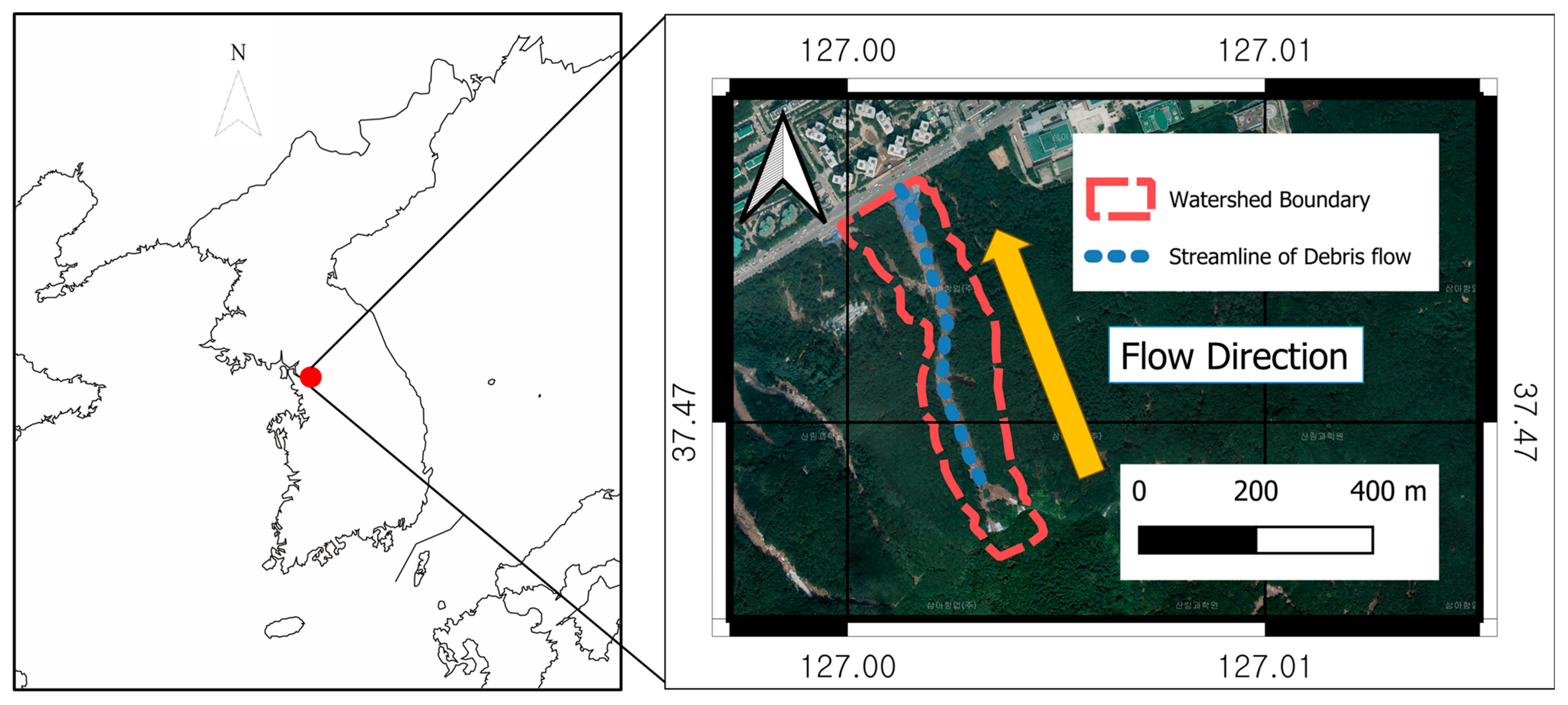
2.1. Study Site

We simulated debris flow on Mt. Umyeon in Seoul in 2011. On 27 July 2011, 151 landslides and 33 debris flows occurred simultaneously, owing to heavy rainfall on Mt. Umyeon, resulting in 16 fatalities [31]. This study focused on the debris flow of the Raemian watershed, for which information on the flow velocity is available (Figure 1). The watershed area is 75,600 m², with an average slope of 44° at the source area, 19° at the flow path, and a maximum flow length of 606.7 m [32]. Field investigations conducted shortly after the event indicated that the debris flow in this watershed was a landslide-induced debris flow, where a landslide in the upper region evolved into a debris flow and entrained channel-bed materials during the flow process. According to Lee et al. [18], the volume of the collapsed sediment evaluated using orthophotographs was 3580 m²; however, the total sediment outflow eventually increased to an estimated 46,125 m³. Although the actual flow velocity and depth were not measured because of the lack of monitoring systems, analysis using CCTV video and field surveys indicated that the maximum flow velocity was approximately 28 m s⁻¹ [32].

Regarding the disaster history, according to field investigations [32], landslide-induced colluvial layers were observed upstream, but the exact timing of the landslide occurrence remains unknown. Notably, DEMs from 2006 and 2009, which are available for the region, show no traces of landslides, suggesting that the landslide likely occurred prior to this period. Moreover, there is no evidence or record of debris flow in this watershed in the past. Meanwhile, debris flows often cause avulsion, forming new pathways as a result of their strong momentum [33]. However, the debris flow in this study followed the stream path detected in the DEMs from 2006 and 2009, indicating no evidence of avulsion.

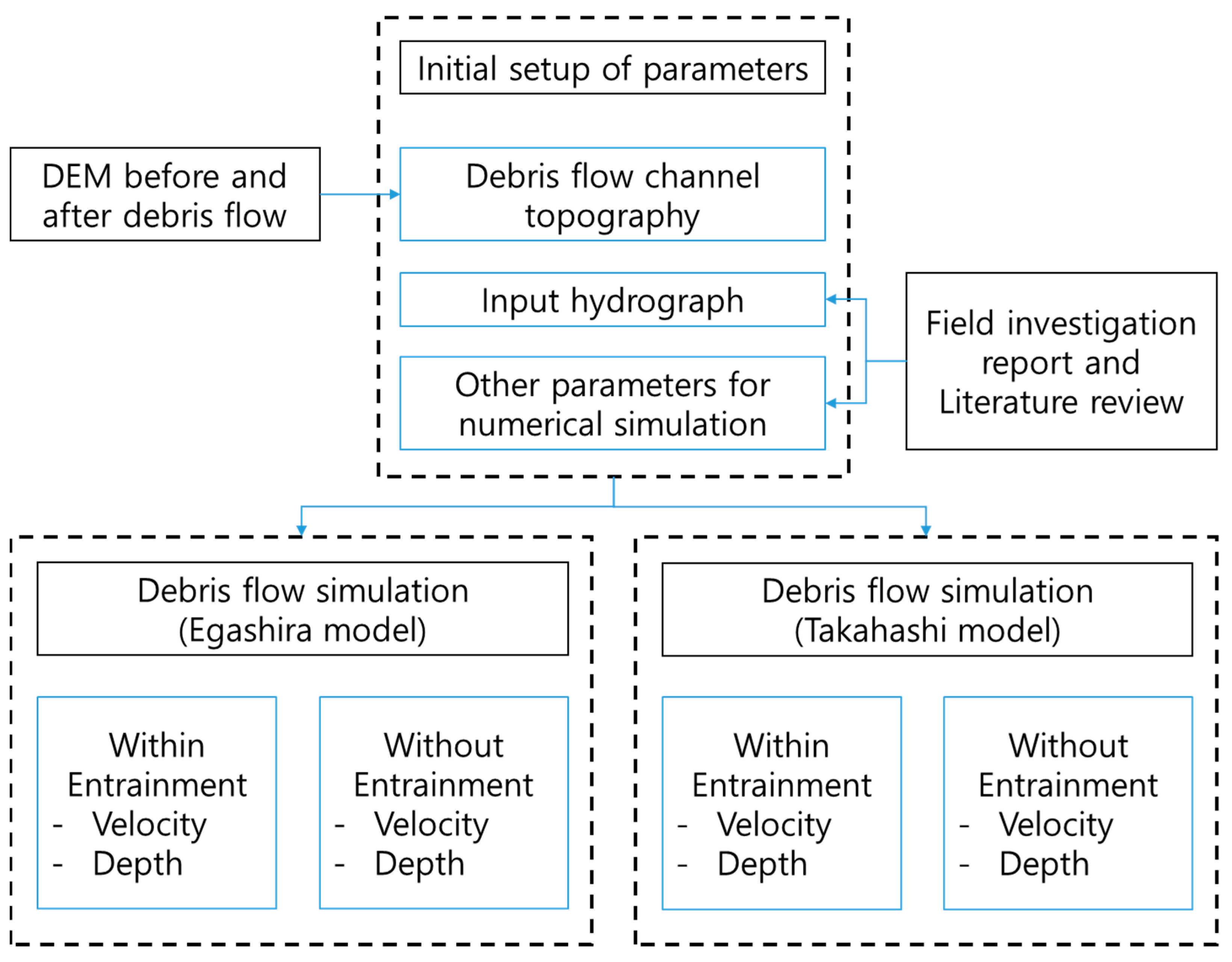
2.2. Debris-Flow Simulation

We conducted numerical simulations of the Raemian watershed debris flow in 2011 using two one-dimensional models, comparing the flow characteristics with and without entrainment terms in each numerical model. The overall process is illustrated in Figure 2.

2.2.1. Governing Equation

The debris flow in the Raemian watershed follows a single straight channel with minimal curvature. This means that this debris flow exhibits dominant flow characteristics of the profile direction compared to that of the cross-direction [34]. Considering this condition, we conducted a one-dimensional analysis because a one-dimensional model can sufficiently reproduce the fluid flow, even with abrupt changes in the cross-sectional shape [35]. To compare the differences in debris-flow characteristics based on the entrainment mechanism, we selected two debris-flow models that include the entrainment model suggested by Egashira et al. [23] (Egashira model) and Takahashi and Nakagawa [28] (Takahashi model).

In terms of the governing equations, the continuity equations of both models are expressed as Equations (1) and (2). As debris flow is a mixture of sediment and water, Equation (2) was applied to account for the change in the sediment content:

$${\displaystyle \frac{\partial h}{\partial t}}+{\displaystyle \frac{\partial Uh}{\partial x}}={\displaystyle \frac{\partial z}{\partial t}}$$

(1)

$${\displaystyle \frac{\partial Ch}{\partial t}}+{\displaystyle \frac{\partial CUh}{\partial x}}=C_{*}{\displaystyle \frac{\partial z}{\partial t}}$$

(2)

where h is the flow depth, U is the depth-averaged flow velocity, z is the bed elevation, C is the depth-averaged volumetric sediment concentration, and C_* is the volumetric sediment concentration in the erodible bed layer.

However, there are differences between the two models in terms of their equations of motion and entrainment mechanisms. In the case of equations of motion, the Egashira model distinguishes between the non-Newtonian stress of debris flow as Coulomb friction on the bed surface (τ_s) and the shear stress due to particle collisions and turbulence (τ_{d and f}) [23]. However, the Takahashi model does not apply separated frictional resistance. The entrainment models also differ. The Egashira model exhibits a continuous change in entrainment rates based on the concentration and slope of the debris flow, whereas the Takahashi model separately applies empirical coefficients for erosion and deposition rates. Equations (3) and (4) and Equations (5)–(7) represent the equations of motion and entrainment terms for the Egashira model, respectively. The Takahashi model comprises the equations of motion (Equations (8) and (9)) and the entrainment model (Equation (10)):

$${\displaystyle \frac{\partial Uh}{\partial t}}+\beta {\displaystyle \frac{\partial U\left(Uh\right)}{\partial x}}=gh{\displaystyle \frac{\partial H}{\partial x}}+{\displaystyle \frac{\tau }{{\rho }_m}}$$

(3)

$${\displaystyle \frac{\tau }{{\rho }_m}}={\displaystyle \frac{{\tau }_s+{\tau }_{d and f}}{{\rho }_m}}=sgn\left(U\right)C(\sigma -\rho )gh\mathit{cos}\theta \mathit{tan}\varphi +{\displaystyle \frac{25}{4}}(k_d\left(1-e^2\right)\sigma C^{{\displaystyle \frac{1}{3}}}+k_f{\displaystyle \frac{{(1-C)}^{5/3}}{C^{2/3}}}\rho ){\left(\frac{d}{h}\right)}^{2}U\left|U\right|$$

(4)

$${\displaystyle \frac{\partial z}{\partial t}}=C_{e}U\mathit{tan}(\theta -{\theta }_e)$$

(5)

$$C_e={\displaystyle \frac{\rho \mathit{tan}\theta }{(\sigma -\rho )(\mathit{tan}\varphi -\mathit{tan}\theta )}}$$

(6)

$${\theta }_e={\mathit{tan}}^{-1}\left({\displaystyle \frac{C(\sigma -\rho )\mathit{tan}\varphi }{C\left(\sigma -\rho \right)+\rho }}\right)$$

(7)

$${\displaystyle \frac{\partial U}{\partial t}}+U{\displaystyle \frac{\partial U}{\partial x}}=g\mathit{sin}\theta -{\displaystyle \frac{\tau }{\rho h}}$$

(8)

$${\displaystyle \frac{\tau }{\rho h}}=\left\{\begin{array}{cc}{\displaystyle \frac{U\left|U\right|d^2}{8h^3\left\{C+\left(1-C\right)\frac{\rho }{\sigma }\right\}\left\{{\left(\frac{C_{*}}{C}\right)}^{\frac{1}{3}}-1\right\}}}& \left(C>0.40C_{*}\right)\\ {\displaystyle \frac{U\left|U\right|d^2}{0.49h^3}}& (0.01<C<0.4C_{*})\end{array}\right.$$

(9)

$${\displaystyle \frac{\partial z}{\partial t}}=\left\{\begin{array}{c}{\delta }_d{\displaystyle \frac{C_e-C}{C_{*}}}U \left({\displaystyle \frac{\partial z}{\partial t}}<0\right) deposition\\ {\delta }_e{\displaystyle \frac{C_e-C}{C_{*}-C_e}}U \left({\displaystyle \frac{\partial z}{\partial t}}\ge 0\right) erosion\end{array}\right. (0.3\le C_e\le 0.9C_{*})$$

(10)

where β (1.25, [36]) is the momentum correction coefficient, g is the gravitational acceleration, H (z + h) represents the total head at the free surface of the debris flow, ρ_m is the debris-flow density, and τ is the non-Newtonian stress term of the debris flow. τ_s is the Coulomb friction acting on the bed surface, whereas τ_{d and f} represent the shear resistance due to particle collisions and turbulence of the interstitial fluid, respectively. θ is the bed slope, σ is the particle density of the sediment, ρ is the density of the interstitial fluid, ϕ is the internal friction angle of the channel bed, e is the restitution coefficient of the debris particles, d is the mean diameter of the particles in the debris flow, k_d is the energy dissipation coefficient due to particle collisions (0.0828, [36]), and k_f is the energy dissipation coefficient due to the turbulence of the interstitial fluid (0.16–0.25, [36]). C_e is the equilibrium volumetric sediment concentration for a given slope. θ_e is the slope at which the specific sediment concentration reaches the equilibrium. In Equation (10), δ_d and δ_e are the deposition and erosion rate coefficients, respectively.

Numerical calculations were performed using the one-dimensional finite difference method for the governing equations of the Egashira and Takahashi models. In this process, the upwind and staggered grid schemes were applied. More detailed numerical schemes are explained in Eu [34].

2.2.2. Parameters Settings

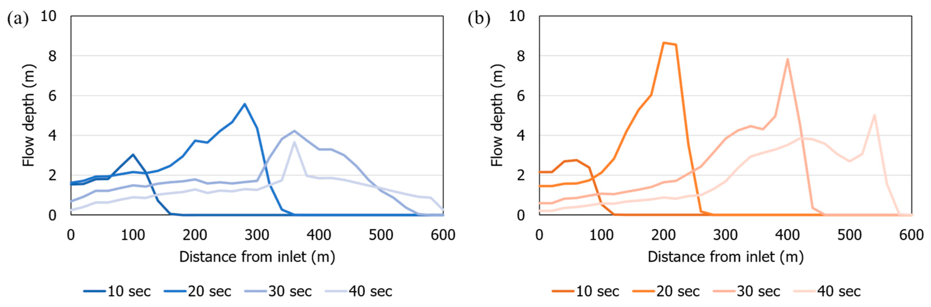
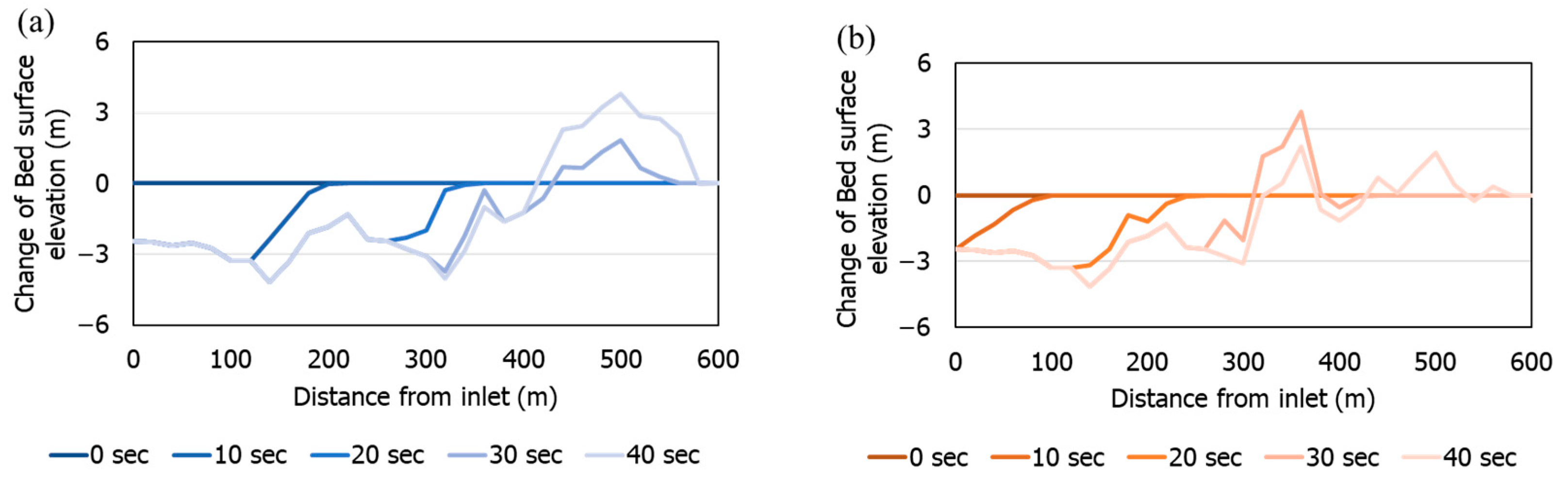
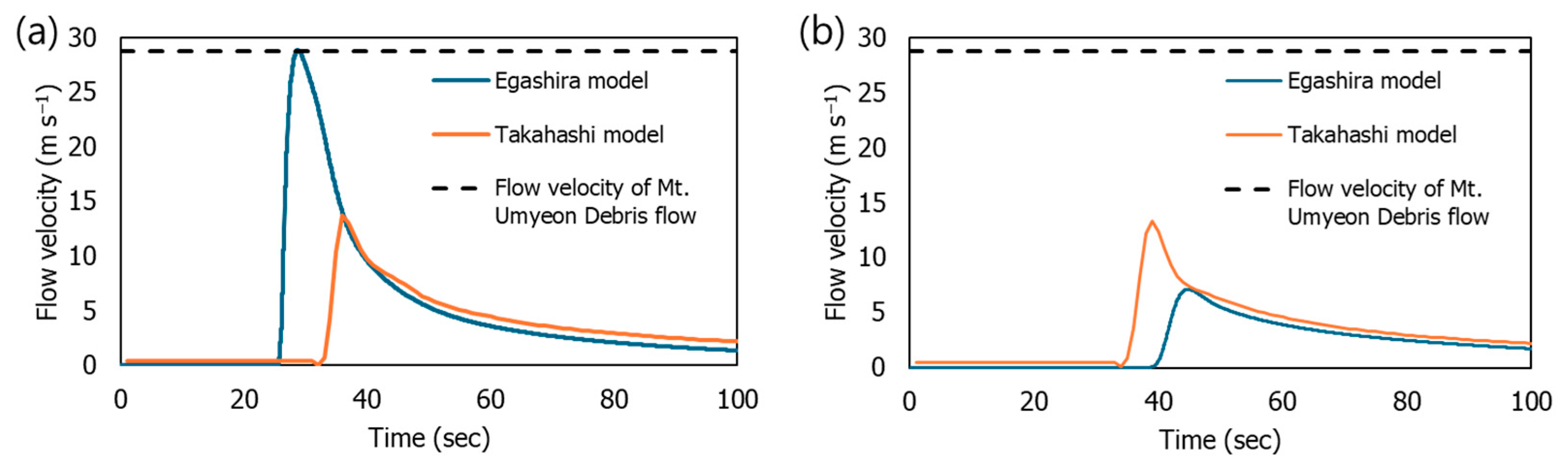
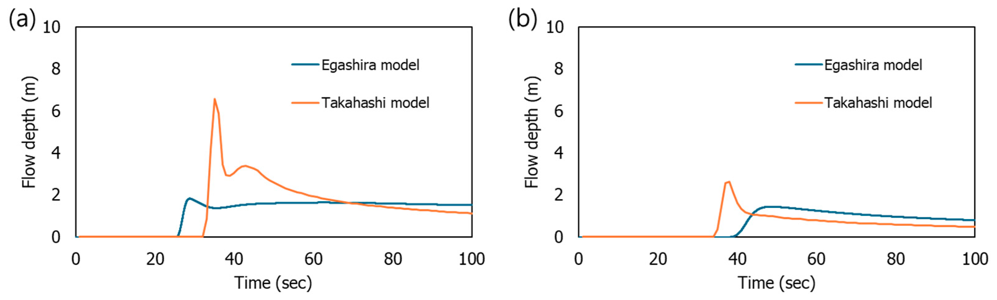
We applied the vertical profile of the debris-flow channel based on DEM data before (January 2009) and after (August 2011) the debris flow using airborne LiDAR at 20 m intervals, according to a field investigation report [32] (Figure 3a). The difference in DEM ranged from 0.83 m to 4.05 m, showing a mean value of 1.65 m. Regarding the channel width, the investigation reported that the stream width was 30 m in the upstream section and widened to 40 m at approximately 360 and 380 m downstream [32]. Therefore, we set the channel width to 30 m, 360 m, and 40 m after 400 m, with a gradual widening section between 360 and 400 m (Figure 3b).

It is challenging to input an accurate value for the initial flow conditions because of the lack of real-time observational data. The sediment volume fraction is generally inferred from the ratio of the mean sediment deposit depth to the mean flow marker depth when no direct observation data is available [37]. However, information regarding the flow marker depth could not be obtained from the field investigation reports and photographs at the time. Due to insufficient direct observational data and indirect evidence, the initial sediment concentration is very ambiguous. Meanwhile, numerical back-analysis conducted in field investigation reports [32] and previous studies [18] suggest that this debris-flow case seems solid-dominated, with a relatively higher solid volume fraction (0.35–0.52). Therefore, we estimated the input hydrograph based on the results of the field investigations [32] and previous studies [18]. The debris-flow density measured immediately after the event was 1886.41 kg m⁻³, and the particle density was approximately 2600 kg m⁻³ [38]. Regarding interstitial fluid density, several studies [39,40] have indicated that some fine particles exhibit phase-shift behavior as fluids. Moreover, previous studies on debris flows in Gangwon Province [41,42] have also successfully simulated debris-flow characteristics using an interstitial fluid density of 1200 kg m⁻³, which is larger than the density of water (1000 kg m⁻³). Although the amount of phase-shifted fine particles was uncertain, we applied an interstitial fluid density of 1200 kg m⁻³, resulting in an initial volume of 17,378 m³, with a 0.206 sediment concentration.

Meanwhile, debris flows in the Raemian watershed occurred over a very short duration. Lee et al. [18] reported that a simulation time of approximately 50 s was sufficient to reproduce a debris-flow event. However, since there are no records of the hydrograph for the initial flow during the event, we applied a triangular hydrograph, which is widely used in previous studies [28,42,43], and it was set that the peak discharge of 1158.57 m³ s⁻¹ occurred 15 s after the event.

The total computation time was set to 100 s, and the space interval was set to 20 m based on the cross-sectional survey intervals of the field investigation [32]. For the time step, a value of 0.01 s was applied to satisfy the Courant–Friedrichs–Lewy (CFL) condition [44], ensuring the stability of the finite difference method. The other parameters were set based on field investigations and previous studies, as listed in

Table 1. Summary of parameters and values used for the debris-flow simulations.

Parameter [Unit]	Symbol	Value	Reference
Internal friction angle (°)	Φ	0.50	[32]
Particle density (kg m−3)	Σ	2600	[32]
Restitution coefficient	e	0.8	[23]
Momentum correction coefficient	β	1.25	[23]
Erosion rate coefficient	δe	0.0007	[20]
Deposition rate coefficient	δd	0.05	[20]
Mean diameter of sediments [m]	d	0.2	[32]

.

3. Results

The results of the 2011 Mt. Umyeon debris-flow simulation using the Egashira and Takahashi models are shown in Figure 4. In the case of the Egashira model, the debris flow rapidly eroded the stream bed after initiation. It reached the outlet after 35.1 s, and sediments were deposited in the lower reaches, which had gentle slopes. The maximum velocity was 28.8 m s⁻¹ at 28.7 s 120 m upstream from the outlet, and the flow depth at that time was 1.84 m. Considering that the maximum debris-flow velocity was 28 m s⁻¹, the Egashira model seems to reproduce this well.

By contrast, the Takahashi model required 42 s to reach the outlet. The maximum velocity and flow depth were 24.33 m s⁻¹ at 24 s at 260 m and 12.04 m at 25 s at 320 m downstream. Meanwhile, 120 m upstream from the outlet, where the Egashira model showed the maximum velocity, the Takahashi model simulated 13.77 m s⁻¹ of the maximum velocity and a flow depth of 6.59 m at 36 s. As the estimated debris-flow velocity in this watershed was based on video footage taken downstream, the results of the Egashira model were considered to represent the actual debris flow on Mt. Umyeon more accurately.

When comparing the Egashira and Takahashi models, the Egashira model showed a very rapid velocity, with a relatively small increase in the flow depth. However, 400 m downstream, where the channel width widens, the flow depth decreased, and the velocity increased drastically. In contrast, the Takahashi model exhibited a characteristic where a distinct debris-flow front continuously appeared. Although the velocity was relatively slow, deeper flow depths were observed. Notably, there was little change in the waveform, despite the gentle slope and expanded channel width in the lower reach.

Regarding changes in the erodible bed (Figure 5), the Egashira model showed concentrated deposition in the lower reach, with the highest deposit height of 3.79 m at 500 m from the inlet. However, the Takahashi model showed a deposit height of 2.22 m 360 m from the inlet, indicating significant deposition in the middle of the channel, whereas relatively little deposition occurred downstream.

To analyze the impact of the entrainment model on the flow characteristics, we compared the cases in which the entrainment model was applied and not applied (∂z/∂t = 0) in both debris-flow models. Except for the entrainment model, all other calculation conditions, such as the input parameters, were identical in this comparison.

Figure 6 and Figure 7 compare the flow velocity and depth of the Egashira and Takahashi models, with and without the application of entrainment, 120 m upstream of the outlet. For the Egashira model, the maximum velocity was 28.8 m s⁻¹ with a flow depth of 1.84 m at 28.7 s when entrainment was considered, while the maximum velocity was 7.13 m s⁻¹ with a flow depth of 1.26 m at 44.8 s without entrainment. Meanwhile, when the entrainment model was applied to the Takahashi model, the maximum velocity of 13.77 m s⁻¹ occurred at 36 s, and the maximum flow depth of 6.59 m was observed at 35 s. Without entrainment, the Takahashi model produced a maximum velocity of 13.32 m s⁻¹ at 39 s and a maximum flow depth of 2.64 m at 38 s.

This indicates that the Egashira model shows a fourfold difference in the maximum velocity, with relatively little difference in the flow depth. In contrast, the Takahashi model showed similar maximum velocities but a 2.5-fold difference in the maximum flow depth. Given the lack of flow depth data and real-time observation data during an actual event, the Egashira model seems to show better results for reproducing the changes in flow characteristics due to entrainment when only velocity is considered.

4. Discussion

Entrainment is a crucial factor in simulating debris flows. Lee et al. [18] simulated debris flow using DAN3D and showed that the flow direction and volume deviated significantly from the observed data without considering entrainment, making it difficult to accurately reproduce the debris flow. Seo [45] compared the sediment yields from initiation and debris-flow channels and the total amount of sediment discharge from the outlet in debris-flow cases in South Korea. This shows that the entrained sediment volume from the debris-flow channel along the stream is critical for determining total sediment discharge. Furthermore, numerous field observations and large-scale flume experiments have reported that entrainment directly affects the mobility of debris flows, allowing them to travel further distances [22,27,46,47]. According to Pudasaini and Fischer [21], entrainment increases the total energy and momentum, owing to the added gravitational load from the eroded mass. In contrast, during deposition, the momentum decreased, owing to the increased frictional resistance on the bed surface and the reduced driving force from the mass decrease.

In this study, the Egashira model showed a fourfold reduction in velocity under conditions without entrainment, indicating that this model could account for the momentum increase due to entrainment. However, the Takahashi model showed little change in debris-flow velocity regardless of whether the entrainment model was applied. This suggests that it does not seem to reflect momentum changes, even when the entrainment model is included. This characteristic might stem from Takahashi’s entrainment mechanism, which relies on the empirically determined erosion and deposition coefficients. Furthermore, owing to differences in the governing equations, the Egashira model interprets an increase in sediment concentration due to entrainment as an increase in momentum induced by increased flow velocity, whereas in the Takahashi model, increased sediment concentration from entrainment results in decreased momentum, which limits the velocity increase and contributes to an increase in flow depth. Consequently, the Egashira model appears to capture momentum changes better than the Takahashi model, owing to entrainment.

In conclusion, when comparing the results of the Egashira and Takahashi models, the Egashira model appears more suitable for simulating debris flows that travel quickly over short distances, as in the case of the debris flow in this study. Although the Egashira model is an empirical model based on Japanese debris-flow cases, it seems to be relatively applicable because its formulation is based on energy slope and sediment concentration relationships, allowing it to be applied without empirical coefficient adjustments. However, as noted by Iverson and Ouyang [26], empirical entrainment models, such as Egashira’s entrainment model, may not be sufficient to express the mechanics of actual entrainment processes in terms of physical interpretation. Recent studies [24,25,26,30] have proposed various physically rigorous entrainment models that utilize more observable parameters, and it is necessary to examine the applicability of these models through further analysis.

This study focused only on analyzing the initial entrainment behavior of debris flows. Generally, debris flows consist of a head of coarse grains or boulders, followed by a liquefied tail that consists of a mixture of finer sediments with a higher water content [1,48]. Additionally, as Shen et al. [30] pointed out, continuous rainfall may lead to additional erosion due to after-flooding. In the case of the debris flow analyzed in this study, field observations showed erosion along the entire 600 m calculation domain, eroding 32,849 m³ of sediment volume, as shown in Figure 3a. However, the simulation results using the Egashira and Takahashi models indicate deposition up to approximately 200 m upstream of the outlet. The estimated eroded and deposited sediment volumes from the Egashira model were 23,936 m³ and 18,767 m³, and 21,212 m³ and 13,504 m³ from the Takahashi model. In this study, we could not conduct a continuous flooding simulation after the initial debris flow passed because of insufficient flood discharge data. However, given that rainfall of at least 68.5 mm continued following the initial debris flow on 27 July 2011, additional erosion due to subsequent runoff could have occurred in this case. Therefore, it is essential to consider erosion due to debris flow, followed by flooding after a debris-flow event, for a more precise comparison of entrainment characteristics.

This study has several limitations. First, we analyzed the effect of entrainment using only a single debris flow. Moreover, the entrainment models applied in this study were derived empirically. Thus, from the results of this study, it is hard to explain the entrainment mechanisms from a general perspective. To address this issue, further studies should be conducted by applying physical-based entrainment models involving field observations and experiments on various debris-flow phenomena.

Additionally, while the debris flow in this study was simplified to a single straight channel for one-dimensional analysis, actual debris flows typically occur in valleys with complex geomorphic conditions. Even in straight channels, the spatial heterogeneity of channel-bed and bank materials makes it challenging to analyze entrainment characteristics using a simple one-dimensional model. Furthermore, numerous researchers have successfully reproduced debris-flow entrainment characteristics using two-dimensional or higher-dimensional models, comparing the results across various approaches [19,25,37]. For instance, Lee et al. [19] conducted an analysis that simultaneously considered both rheological and entrainment models. Although previous studies have focused on determining the most appropriate entrainment model for accurately reproducing debris flows, they also offer valuable insights into how the inclusion or exclusion of entrainment mechanisms influences debris-flow dynamics. Therefore, it is essential to conduct two-dimensional or higher-dimensional spatial analyses to capture spatial heterogeneity and improve the understanding of debris-flow dynamics.

Accurate parameter estimation is also crucial for precise debris-flow simulation, particularly for the inflow hydrograph and initial sediment concentration, which significantly affect downstream debris-flow characteristics. Moreover, the parameters used in the simulation should be calibrated and validated based on actual debris-flow data. However, information on the initial stage of debris flow or real-time flow characteristics was not measured, and the available data were obtained only after the event. Thus, the initial parameter setup based on field investigation, such as geotechnical variables, might be significantly different from the condition of real debris flow, resulting in a discrepancy between the simulation and the real case. Given the close relationship between the initial sediment concentration and entrainment on the channel bed, precise estimation methods are required for the initial runoff and sediment volume when reproducing or predicting debris-flow behavior.

5. Conclusions

This study analyzed the impact of entrainment on debris-flow numerical simulations by reproducing a debris-flow case using two types of one-dimensional debris-flow models and comparing the influence of entrainment. The analysis shows that the estimated flow velocity and depth varied depending on the entrainment model in each simulation and that the Egashira model more accurately reproduced the debris-flow case in this study. Notably, the analysis results for conditions without entrainment did not effectively reproduce the actual flow characteristics of debris flow. This indicates that including an entrainment model is essential for reasonably simulating debris-flow characteristics, such as flow velocity.

Although this study highlights the importance of entrainment models in replicating debris-flow characteristics, the results of this study are difficult to apply to other debris-flow cases or to suggest an optimized entrainment model because we focused on analyzing the reproduction conditions for a specific event using a simple one-dimensional model and examining only two types of entrainment models. Future improvements to entrainment models and expansion to two-dimensional analyses to reproduce deposit fan formations could enable accurate predictions of debris-flow impact areas, providing a tool for effective hazard zonation for warning and evacuation planning in response to debris flows.

References

1. Hungr, O.; Evans, S.; Bovis, M.; Hutchinson, J. A review of the classification of landslides of the flow type. Environ. Eng. Geosci. 2001, 7, 221–238. [Google Scholar] [CrossRef]
2. Takahashi, T. Debris Flow: Mechanics, Prediction and Countermeasures, 2nd ed.; CRC Press/Balkema: Leiden, The Netherlands, 2014. [Google Scholar]
3. Dowling, C.A.; Santi, P.M. Debris flows and their toll on human life: A global analysis of debris-flow fatalities from 1950 to 2011. Nat. Hazards 2014, 71, 203–227. [Google Scholar] [CrossRef]
4. Hu, K.; Wei, F.; Li, Y. Real-time measurement and preliminary analysis of debris-flow impact force at Jiangjia Ravine, China. Earth Surf. Process. Landf. 2011, 36, 1268–1278. [Google Scholar] [CrossRef]
5. Jakob, M. Debris-flow hazard analysis. In Debris-flow Hazards and Related Phenomena; Jacob, M., Hungr, O., Eds.; Springer: Berlin/Heidelberg, Germany, 2005; pp. 411–443. [Google Scholar]
6. Guzzetti, F.; Gariano, S.L.; Peruccacci, S.; Brunetti, M.T.; Marchesini, I.; Rossi, M.; Melillo, M. Geographical landslide early warning systems. Earth-Sci. Rev. 2020, 200, 102973. [Google Scholar] [CrossRef]
7. Piciullo, L.; Calvello, M.; Cepeda, J.M. Territorial early warning systems for rainfall-induced landslides. Earth-Sci. Rev. 2018, 179, 228–247. [Google Scholar] [CrossRef]
8. Hübl, J.; Suda, J.; Proske, D.; Kaitna, R.; Scheidl, C. Debris flow impact estimation. In Proceedings of the 11th International Symposium on Water Management and Hydraulic Engineering, Ohrid, Macedonia, 1–5 September 2009; pp. 1–5. [Google Scholar]
9. Scheidl, C.; Chiari, M.; Kaitna, R.; Mullegger, M.; Krawtschuk, A.; Zimmermann, T.; Proske, D. Analysing Debris-Flow Impact Models, Based on a Small Scale Modeling Approach. Surv. Geophys. 2013, 34, 121–140. [Google Scholar] [CrossRef]
10. Korea Forest Service. Landslide Information System. Available online: https://sansatai.forest.go.kr/ (accessed on 17 November 2024).
11. Armanini, A. On the dynamic impact of debris flows. In Recent Developments on Debris Flows; Armanini, A., Michiue, M., Eds.; Springer: Berlin/Heidelberg, Germany, 1997; Volume 64, pp. 208–226. [Google Scholar]
12. Canelli, L.; Ferrero, A.M.; Migliazza, M.; Segalini, A. Debris flow risk mitigation by the means of rigid and flexible barriers—Experimental tests and impact analysis. Nat. Hazards Earth Syst. Sci. 2012, 12, 1693–1699. [Google Scholar] [CrossRef]
13. Hungr, O.; Morgan, G.; Kellerhals, R. Quantitative analysis of debris torrent hazards for design of remedial measures. Can. Geotech. J. 1984, 21, 663–677. [Google Scholar] [CrossRef]
14. Lo, D.O.K. Review of Natural Terrain Landslide Debris-Resisting Barrier Design; Geotechnical Engineering Office, Civil Engineering Department: Hong Kong, China, 2000.
15. National Institute for Land and Infrastructure Management. Manual of Technical Standard for Designing Sabo Facilities Against Debris Flow and Driftwood; National Institute for Land and Infrastructure Management: Tsukuba, Japan, 2016.
16. Christen, M.; Kowalski, J.; Bartelt, P. RAMMS: Numerical simulation of dense snow avalanches in three-dimensional terrain. Cold Reg. Sci. Technol. 2010, 63, 1–14. [Google Scholar] [CrossRef]
17. George, D.L.; Iverson, R.M. A depth-averaged debris-flow model that includes the effects of evolving dilatancy. II. Numerical predictions and experimental tests. Proc. R. Soc. A Math. Phys. Eng. Sci. 2014, 470, 20130820. [Google Scholar] [CrossRef]
18. Lee, D.-H.; Lee, S.R.; Park, J.-Y. Numerical Simulation of Debris Flow Behavior at Mt. Umyeon using the DAN3D Model. J. Korean Soc. Hazard Mitig. 2019, 19, 195–202. [Google Scholar] [CrossRef]
19. Lee, S.; An, H.; Kim, M.; Lee, G.; Shin, H. Evaluation of different erosion–entrainment models in debris-flow simulation. Landslides 2022, 19, 2075–2090. [Google Scholar] [CrossRef]
20. Nakatani, K.; Wada, T.; Satofuka, Y.; Mizuyama, T. Development of “Kanako 2D (Ver. 2.00),” a user-friendly one-and two-dimensional debris flow simulator equipped with a graphical user interface. Int. J. Eros. Control Eng. 2008, 1, 62–72. [Google Scholar] [CrossRef]
21. Pudasaini, S.P.; Fischer, J.-T. A mechanical erosion model for two-phase mass flows. Int. J. Multiph. Flow 2020, 132, 103416. [Google Scholar] [CrossRef]
22. Reid, M.E.; Iverson, R.M.; Logan, M.; LaHusen, R.G.; Godt, J.W.; Griswold, J.P. Entrainment of bed sediment by debris flows: Results from large-scale experiments. In Proceedings of the Fifth International Conference on Debris-Flow Hazards Mitigation, Mechanics, Prediction and Assessment, Editrice Universita La Sapienza, Rome, Italy, 14–17 June 2011; pp. 367–374. [Google Scholar]
23. Egashira, S.; Honda, N.; Itoh, T. Experimental study on the entrainment of bed material into debris flow. Phys. Chem. Earth Part C Sol. Terr. Planet. Sci. 2001, 26, 645–650. [Google Scholar] [CrossRef]
24. Frank, F.; McArdell, B.W.; Huggel, C.; Vieli, A. The importance of entrainment and bulking on debris flow runout modeling: Examples from the Swiss Alps. Nat. Hazards Earth Syst. Sci. 2015, 15, 2569–2583. [Google Scholar] [CrossRef]
25. Han, Z.; Chen, G.; Li, Y.; Tang, C.; Xu, L.; He, Y.; Huang, X.; Wang, W. Numerical simulation of debris-flow behavior incorporating a dynamic method for estimating the entrainment. Eng. Geol. 2015, 190, 52–64. [Google Scholar] [CrossRef]
26. Iverson, R.M.; Ouyang, C. Entrainment of bed material by Earth-surface mass flows: Review and reformulation of depth-integrated theory. Rev. Geophys. 2015, 53, 27–58. [Google Scholar] [CrossRef]
27. McDougall, S.; Hungr, O. Dynamic modeling of entrainment in rapid landslides. Can. Geotech. J. 2005, 42, 1437–1448. [Google Scholar] [CrossRef]
28. Takahashi, T.; Nakagawa, H. Prediction of Stony Debris Flow Induced by Severe Rainfall. J. Jpn. Soc. Eros. Control Eng. 1991, 44, 12–19. [Google Scholar]
29. Denlinger, R.P.; Iverson, R.M. Flow of variably fluidized granular masses across three-dimensional terrain: 2. Numerical predictions and experimental tests. J. Geophys. Res. Solid Earth 2001, 106, 553–566. [Google Scholar] [CrossRef]
30. Shen, P.; Zhang, L.; Wong, H.F.; Peng, D.; Zhou, S.; Zhang, S.; Chen, C. Debris flow enlargement from entrainment: A case study for comparison of three entrainment models. Eng. Geol. 2020, 270, 105581. [Google Scholar] [CrossRef]
31. Jeong, S.; Kim, Y.; Lee, J.K.; Kim, J. The 27 July 2011 debris flows at Umyeonsan, Seoul, Korea. Landslides 2015, 12, 799–813. [Google Scholar] [CrossRef]
32. Seoul Metropolitan Goverment. Supplimentary Investigation of Cause of Mt. Umyeon Landslide; Seoul Metropolitan Goverment: Seoul, Republic of Korea, 2014.
33. Schiavo, M.; Gregoretti, C.; Boreggio, M.; Barbini, M.; Bernard, M. Probabilistic identification of debris-flow pathways in mountain fans within a stochastic framework. J. Geophys. Res. Earth Surf. 2024, 129, e2024JF007946. [Google Scholar] [CrossRef]
34. Eu, S. Long-Term Stability Analysis of Erosion Control Dam Considering Debris-Flow Entrainment Impact Force Simulation. Doctoral Dissertation, Seoul National University, Seoul, Republic of Korea, 2020. [Google Scholar]
35. Cueto-Felgueroso, L.; Santillán, D.; García-Palacios, J.H.; Garrote, L. Comparison between 2D shallow-water simulations and energy-momentum computations for transcritical flow past channel contractions. Water 2019, 11, 1476. [Google Scholar] [CrossRef]
36. Egashira, S. Stoppage and Deposition Mechanism of Debris Flow (2). J. Jpn. Soc. Eros. Control Eng. 1993, 46, 51–56. [Google Scholar]
37. Barnhart, K.R.; Jones, R.P.; George, D.L.; McArdell, B.W.; Rengers, F.K.; Staley, D.M.; Kean, J.W. Multi-model comparison of computed debris flow runout for the 9 January 2018 Montecito, California post-wildfire event. J. Geophys. Res. Earth Surf. 2021, 126, e2021JF006245. [Google Scholar] [CrossRef]
38. Seoul Metropolitan Goverment. Mt. Umyeon Lansdlide Recovery Plan. Lot No.1: Raemian, Imgwang and Jeonwon Area; Seoul Metropolitan Government: Seoul, Republic of Korea, 2012.
39. Nishiguchi, Y.; Uchida, T. Long-runout-landslide-induced debris flow: The role of fine sediment deposition processes in debris flow propagation. J. Geophys. Res. F Earth Surf. 2022, 127, e2021JF006452. [Google Scholar] [CrossRef]
40. Uchida, T.; Nishiguchi, Y.; Nakatani, K.; Satofuka, Y.; Yamakoshi, T.; Okamoto, A.; Mizuyama, T. New numerical simulation procedure for large-scale debris flows (Kanako-LS). Int. J. Eros. Control Eng. 2013, 6, 58–67. [Google Scholar] [CrossRef]
41. Jang, S. Sediment-Related Disaster Risk Assessment by the Use of Physically-Based Models Considering the Effect of Tree Roots on Soil Reinforcement in a Forested Catchment. Doctoral Dissertation, Kangwon National University, Chuncheon, Republic of Korea, 2019. [Google Scholar]
42. Lim, Y.-H. A Study on the Application of Numerical Simulation to Erosion Control Facility using KANAKO 2D. Doctoral Dissertation, Kangwon National University, Chuncheon, Republic of Korea, 2017. [Google Scholar]
43. Liu, J.; Nakatani, K.; Mizuyama, T. Effect assessment of debris flow mitigation works based on numerical simulation by using Kanako 2D. Landslides 2013, 10, 161–173. [Google Scholar] [CrossRef]
44. Courant, R.; Friedrichs, K.; Lewy, H. On the partial difference equations of mathematical physics. IBM J. Res. Dev. 1967, 11, 215–234. [Google Scholar] [CrossRef]
45. Seo, J.; Woo, C.; Lee, C.; Kim, D. Characteristics of Sediment Discharge Based on GIS Spatial Analysis of Area Damaged by Debris Flow. J. Korean Soc. Hazard Mitig. 2018, 18, 89–96. [Google Scholar] [CrossRef]
46. Godt, J.W.; Coe, J.A. Alpine debris flows triggered by a 28 July 1999 thunderstorm in the central Front Range, Colorado. Geomorphology 2007, 84, 80–97. [Google Scholar] [CrossRef]
47. Rickenmann, D. Runout prediction methods. In Debris-Flow Hazards and Related Phenomena; Jacob, M., Hungr, O., Eds.; Springer: Berlin/Heidelberg, Germany, 2005; pp. 305–324. [Google Scholar]
48. Iverson, R.M. The physics of debris flows. Rev. Geophys. 1997, 35, 245–296. [Google Scholar] [CrossRef]
Figure 1. Location of the Raemian watershed. The red line shows the watershed boundary, and the blue line indicates the debris-flow channel of the watershed.
Water 17 00761 g001
Figure 2. Flow chart of debris-flow simulation conducted in this study.
Water 17 00761 g002
Figure 3. Longitudinal profile (a) and cross-sectional profile (b) of debris-flow channel in Raemian watershed. In (a), to describe change in debris-flow channel topography clearly, differences in elevation between pre- and post-debris-flow events are exaggerated by 5 times.
Water 17 00761 g003
Figure 4. Results of simulated debris-flow propagation using the Egashira (a) and Takahashi (b) models.
Water 17 00761 g004
Figure 5. Results of simulated channel bed surface elevation change using the Egashira (a) and Takahashi (b) models. Zero indicates the original bed elevation before the debris flow, and positive and negative values in the y-axis indicate deposition and erosion, respectively.
Water 17 00761 g005
Figure 6. Maximum flow velocity 120 m upstream from outlet when entrainment model includes (a) and does not include (b).
Water 17 00761 g006
Figure 7. Maximum flow depth at 120 m upstream from the outlet when the entrainment model includes (a) and does not include (b).
Water 17 00761 g007