Research on a DBSCAN-IForest Optimisation-Based Anomaly Detection Algorithm for Underwater Terrain Data

Abstract

The accurate acquisition of underwater topographic data is crucial for the representation of river morphology and early warning of water hazards. Owing to the complexity of the underwater environment, there are inevitably outliers in monitoring data, which objectively reduce the accuracy of the data; therefore, anomalous data detection and processing are key in effectively using data. To address anomaly detection in underwater terrain data, this paper presents an optimised DBSCAN-IForest algorithm model, which adopts a distributed computation strategy. First, the K-distance graph and Kd-tree methods are combined to determine the key computational parameters of the DBSCAN algorithm, and the DBSCAN algorithm is applied to perform preliminary cluster screening of underwater terrain data. The isolated forest algorithm is subsequently used to carry out refined secondary detection of outliers in multiple subclusters that were initially screened. Finally, the algorithm performance is verified through example calculations using a dataset of about 8500 underwater topographic points collected from the Yellow River Basin, which includes both elevation and spatial distribution attributes; the results show that compared with other methods, the algorithm has greater efficiency in outlier detection, with a detection rate of up to 93.75%, and the parameter settings are more scientifically sound and reasonable. This research provides a promising framework for anomaly detection in underwater terrain data.

1. Introduction

The accurate acquisition of underwater topographic data is highly important in the depiction of river morphology and early warning of water hazards. The acquisition of this type of data is costly and often requires high-precision measurement equipment, such as single-beam and multibeam sounders and side-scan sonar [1,2]. Owing to the complex monitoring environment in the field, there are inevitably outliers in monitoring data, which affects the overall accuracy; therefore, the detection and processing of outliers in underwater terrain monitoring data are key in the efficient use of such data [3].

Considering the trend of simplicity in monitoring equipment and its increasing popularity, the outliers in terrain monitoring data are affected increasingly little by human operation; they are mainly caused by errors in the monitoring equipment itself and by environmental factors [4,5,6]. There may be problems with monitoring equipment such as inaccurate calibration and equipment failure during the measurement process, resulting in errors in the collected data; environmental factors such as terrain undulation, vegetation cover, and climatic conditions also affect the terrain monitoring data. Outliers in data include isolated points, noise points, and error points, and their presence interferes with the accuracy and reliability of data analysis [7]. Generally, outliers are considered abnormal entities that deviate from the rest of the dataset and are traditionally regarded as singular. However, owing to the random distribution of underwater terrain washout patterns and the sampling characteristics of the temporal sensors that collect the data, population-based regional anomalies may arise, resulting in a variety of distributions for the outliers, such as appearing singly or in clusters. This increases the difficulty of applying traditional anomalous data detection methods to underwater terrain data.

To address the influence of underwater terrain data outliers on data analysis, experts and scholars have conducted much research in the field of bathymetry and have processed underwater terrain data with algorithms such as weighted averages [8], AR models, statistical principles, median filters, uncertainty, and Kalman waves [9] to identify and remove outliers. While existing algorithms have demonstrated a promising performance, they are constrained by several inherent limitations. Traditional approaches struggle to effectively capture complex nonlinear relationships, as seen in autoregressive models. Many methods exhibit high sensitivity to parameter selection, particularly in weighted averaging techniques, while others depend on restrictive assumptions rooted in statistical principles. The challenge of preserving fine-grained details during noise reduction processes remains prevalent, especially in median filtering applications. Furthermore, these approaches often face difficulties in quantifying predictive uncertainty and maintaining robustness against model inaccuracies, a notable issue in Kalman filtering implementations. Moreover, regional outliers may be misjudged and processed as ‘pseudo river core beach’ or ‘pseudo scour pits’. With the development of big data and artificial intelligence technology, more cutting-edge methods have been applied in anomaly data detection [10]; according to the different principles used, the relevant algorithms are divided into qualitative anomaly detection algorithms based on a priori knowledge, quantitative anomaly detection algorithms based on models, and data-driven anomaly detection algorithms. The recognition of anomalous features in complex underwater environments is insufficient [11]; in recent years, the above three types of anomaly recognition algorithms have been further improved [12], and the number of parameter settings used in the computational process has been substantially reduced, which greatly increases the computational efficiency. However, there are still studies that assume that artificial settings must be used for the key parameters in these methods, which is not sufficiently objective. Research on automated and efficient anomaly detection methods has become popular in recent years. Ruichen Zhang et al. [13] proposed a CVAE-GAN network by combining the CVAE and DCGAN for seabed pseudoterrain detection, which increased the detection efficiency and accuracy. Long, Jiawei et al. [14] proposed an unsupervised anomaly detection method based on deep learning by using the PCPNet architecture, which reduced the need for parameter adjustment; however, the above two algorithms are not efficient in regional anomaly identification. In contrast, DBSCAN is well-suited for complex datasets, including underwater terrain data, due to its ability to handle noise and identify clusters of varying densities, making it a robust choice for such applications [15]. Relevant studies have shown [16,17] that regional anomaly determination in underwater 3D spaces is still difficult, and due to the random distribution of underwater terrain, the error in anomaly detection on the basis of a priori knowledge and models is large. Current research focuses on data-driven anomaly detection, integrating advanced data processing technology and artificial intelligence algorithms to improve algorithm robustness, computational efficiency, and adaptability to complex underwater environments [16,17,18] to achieve accurate analysis and anomaly identification for underwater terrain data. In addition, the current research lacks a unified theoretical framework and evaluation standards, and there are difficulties in comparing and validating different methods, which limits the application and development of anomaly detection technology for underwater terrain data.

In summary, at present, there is abundant research on anomaly data detection worldwide, but because of the complexity of underwater terrain data, the efficiency of state-of-the-art methods in underwater terrain anomaly data detection is not high [19,20,21]. Thus, considering practical applications, an optimised DBSCAN-IForest anomaly data recognition model for anomaly detection in underwater terrain data is proposed. The main contributions of this paper are as follows: (1) A method of optimising the DBSCAN algorithm is proposed, which solves the problem of human-set parameters interfering with the results of the algorithm. This method minimises the uncertainty in setting the parameters of the DBSCAN algorithm by considering the specific data characteristics and improves the scientific validity and robustness of the algorithm. (2) A step-by-step screening method is proposed, in which the DBSCAN algorithm is used to carry out preliminary screening, the original data are divided into clusters, and then the IForest algorithm is used to screen the subclusters, which takes full advantage of the two algorithms and improves the efficiency and accuracy of data processing. (3) The algorithm is applied to underwater topographic data measured for the Madu Dangerous Project in the lower reaches of the Yellow River, and the results show that the algorithm has high detection accuracy; the research results provide useful reference data for the detection and processing of anomalous data.

2. Methodology

2.1. DBSCAN Algorithm

The DBSCAN algorithm implements clustering and anomaly detection on the basis of core objects and density reachability by taking a data point as a starting point, specifying the domain radius ε, calculating the number of points in its surrounding neighbourhood, and marking the point as a core object if the number of points is greater than or equal to a prespecified threshold Minpts [16]. For points around a core object, if these points are also core objects, they are density reachable with respect to each other, i.e., they can reach each other and form a cluster. For a noncore object, if it is located within the radius ε of a core object but the number of points around it is less than Minpts, it is considered a boundary point; however, it can still be densely connected to the core object through other core objects and thus classified into the corresponding cluster. Points that cannot reach any core object and are not core objects are regarded as anomalies. As shown in Figure 1.

2.1.1. Calculating the Sensitivity of Parameter Settings

The performance of the DBSCAN algorithm is highly dependent on two parameters, ε and Minpts. ε determines the size of the neighbourhood, whereas Minpts determines the number of points that must exist within the neighbourhood of a point for it to become a core point [17]. In 3D space, choosing the appropriate ε and Minpts is more difficult because of the increased distribution and density complexity of the data. If these parameters are not selected properly, the clustering results may deviate from reality. Therefore, in this study, K-distance plots and Kd-trees are used to calculate the values of these two parameters separately to reduce the influence of these two parameters on the model and increase the model’s stability and reliability. In addition, the uncertainty caused by manual parameter settings is avoided.

2.1.2. Limitations of 3D Data Anomaly Detection

Although the DBSCAN algorithm exhibits some robustness to noisy points, it may incorrectly include anomalous data points in a certain cluster in specific contexts, affecting the accuracy of the detection results. This is a result of its density-based clustering method, which tends to group points with similar densities into the same cluster. In 3D spatial data, the definition of anomalous points is more complex, and these points may have unique density or distribution characteristics, which are often difficult to quantify accurately. Therefore, the DBSCAN algorithm has some limitations in anomaly detection in 3D space. Considering the characteristics of the algorithm, which uses density for detection, in this study, the algorithm is used to divide the 3D data into clusters and perform initial screening, and then each subcluster is finely screened using the isolated forest algorithm.

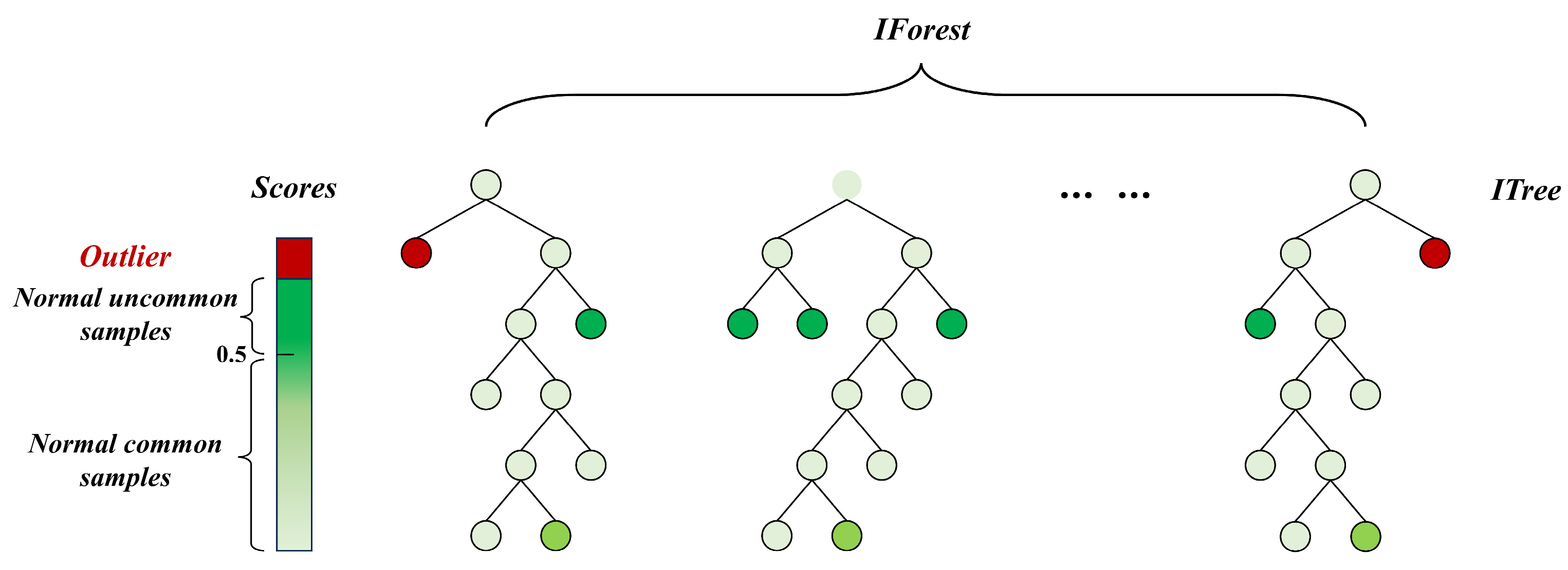
2.2. Isolated Forest Algorithm

The isolated forest algorithm identifies anomalies by constructing multiple randomised decision trees on the basis of isolating data points in the feature space [22]. Each tree randomly selects features and segmentation points and recursively divides the data until a single point or maximum depth is reached. The path length of a data point (the number of splits from the root to the leaf node) reflects its degree of isolation, and short paths are considered anomalous. The results of each tree are combined to calculate the anomaly score and identify anomalous data points. As shown in Figure 2 The formula is as follows:

• where $\mathrm{h}\left(\mathrm{x}\right)$ is the path length of node x in the isolated tree from the root to the leaf node. When the sample size of the dataset is n, the expected value of the average path length of the points $\mathrm{c}\left(\mathrm{n}\right)$ in the isolated tree is [23]

$$\mathrm{c}\left(\mathrm{n}\right)=2\mathrm{H}\left(\mathrm{n}-1\right)-{\displaystyle \frac{2\left(\mathrm{n}-1\right)}{\mathrm{n}}}$$

(1)

where h(i) is the ith summation number, defined as H(i) = ln(i) + y, and y ≈ 0.5772156649, known as the Euler–Marcheroni constant.

The anomaly score s(x, n) is defined as

$$\mathrm{s}\left(\mathrm{x},\mathrm{n}\right)=2^{-{\displaystyle \frac{\mathrm{E}\left(\mathrm{h}\left(\mathrm{x}\right)\right)}{\mathrm{c}\left(\mathrm{n}\right)}}}$$

(2)

E(h(x)) is the average path length of point x in all trees. If s(x, n) is close to 1, x is an anomaly point, and if it is close to 0, it is a normal point.

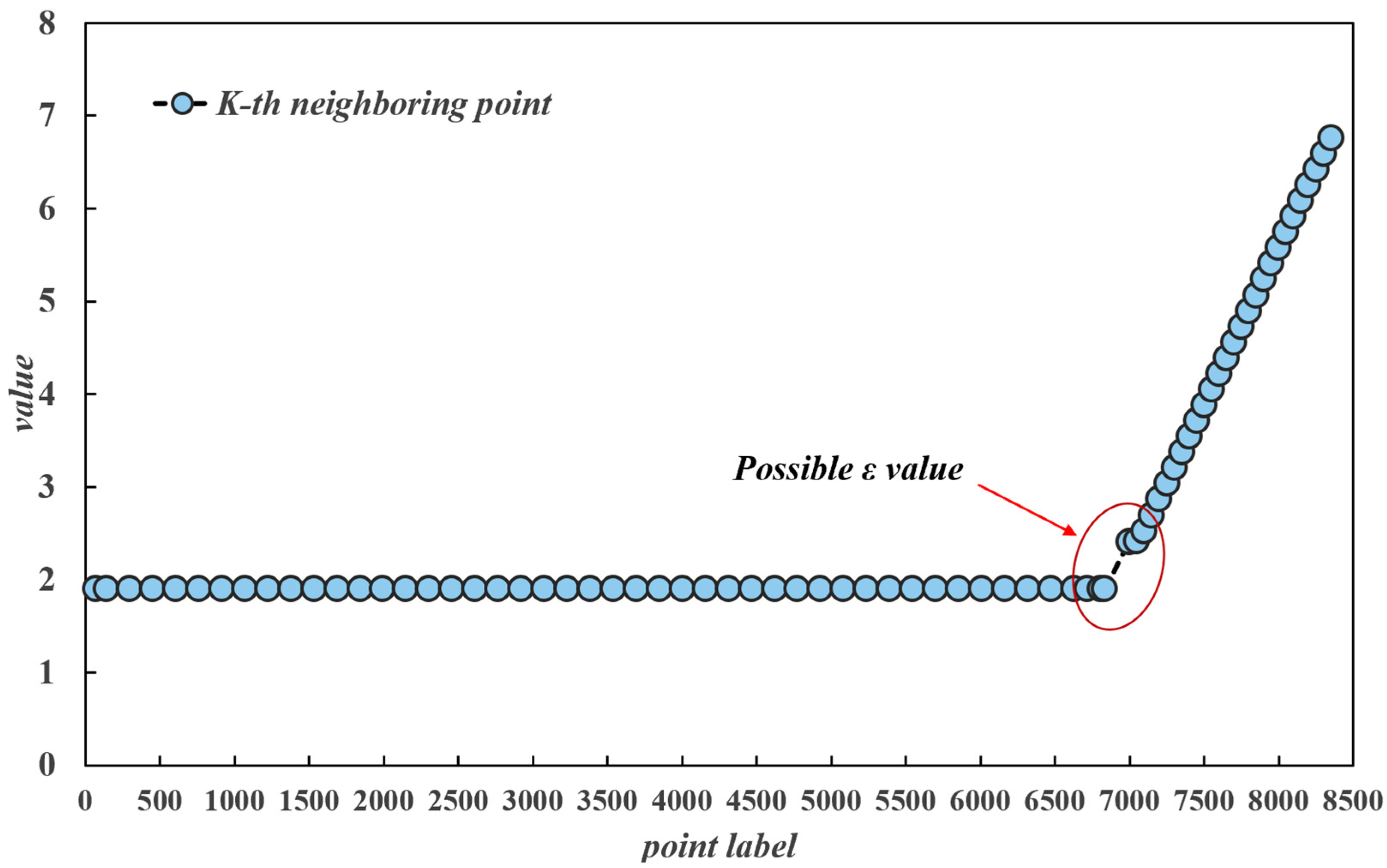
2.3. K-Distance Chart

The K-distance chart represents the local density distribution characteristics of data points by quantifying the distance from each data point in the dataset to its kth nearest neighbour [22]. This method involves calculating, ranking, and visualising the kth distance to the nearest neighbour for each data point in the dataset to represent the statistical distribution pattern of the distance values. In the constructed K-distance plots, the corresponding K-distance changes as the horizontal coordinates increase, which reflects the proximity of the data points to each other in a dense region. When the horizontal coordinate increases to a certain threshold, the K-distance significantly increases; this is known as the ‘inflection point’. This inflection point indicates a change in the local density of the data points, which manifests as a transition from a high-density region to a low-density region. Therefore, the positioning of the inflection point reveals the demarcation of different-density areas in the dataset and provides a scientific basis for establishing a critical threshold for the relative distance between data points.

2.4. Kd-Tree

A Kd-tree is a binary tree structure for organising k-dimensional spatial data, and its construction process consists of three steps: selecting the split axis, selecting the split point and recursively constructing the subtree [24]. Each node corresponds to a k-dimensional data point, and the entire Kd-tree is constructed recursively by dividing the data points into left and right subtrees by selecting appropriate split axes and split points [25].

In constructing the Kd-tree, the recursive division process selects the dimension with the largest variance as the cut-off dimension to equalise the data distribution. After the data points are sorted by this dimension, the midpoint is selected as the split point to ensure that the lengths of the left and right subtree data are the same, dividing the dataset into two subsets. The subsets are subsequently recursively divided using the other dimensions until the number of data points in each subset falls below a preset threshold or until the tree reaches a specified depth. In this process, a hierarchical data structure is constructed in which each node represents a segmentation hyperplane, enabling the efficient indexing of multidimensional spatial data. There are two types of search methods in the Kd-tree structure: range search and K-nearest-neighbour search. Range search refers to the search for point data within a given search threshold for a point object; in K-nearest-neighbour search, a point object is specified, and then the original dataset is traversed to find the k-nearest point data to the point object.

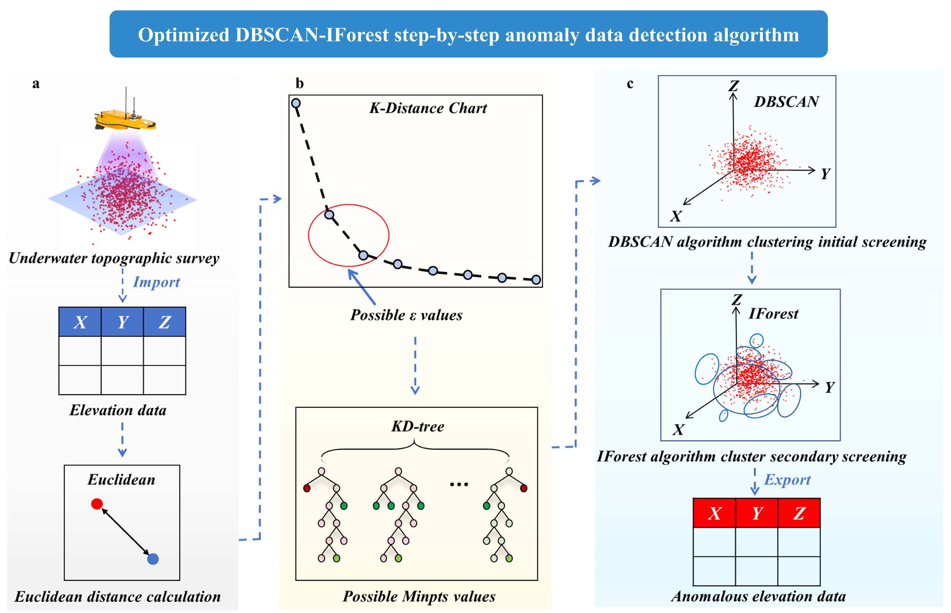
2.5. Constructing the Model for the Anomaly Detection Algorithm for Underwater Terrain Data

As seen from the content of the previous research and analysis, most of the existing methods for detecting anomalies in underwater terrain data require the calculation parameters to be set by humans, and the results are greatly affected by the parameter setting. To reduce the influence of manually set parameters on the detection results, we propose an optimised numerical identification model for anomalies, DBSCAN-IForest, which uses the K-distance graph to determine the neighbourhood radius ε for the DBSCAN algorithm and uses the Kd-tree to select the optimal Minpts; this eliminates the influence of human-set parameters as far as possible. Afterwards, the DBSCAN algorithm is used to screen the data in the first round, divide the data into different subclusters, and mark those that do not meet the screening conditions of the DBSCAN algorithm as anomalies; this method can identify some of the outliers. Then, for each subcluster, the isolated forest algorithm is used to carry out anomaly detection; in particular, it is used for supplementary detection of local outliers that are larger than Minpts. Finally, the anomalies obtained from the detections in the two steps are integrated, and the optimal Minpts value is obtained. The detected anomalies are integrated to obtain the final anomaly detection results.

As shown in Figure 3, the specific steps of model construction are as follows:

(1)

ε parameter determination. For a given dataset, the distance from each data point to its kth nearest neighbour is calculated, and each point in the dataset is traversed, after which the kth-nearest-neighbour distances of all the data points are sorted in ascending order to obtain an ordered distance sequence. The sorted distance sequence is used as the vertical axis of the K-distance graph, and the index of the data points is used as the horizontal axis. Considering that the underwater terrain data are three-dimensional and exist in three-dimensional space, the Euclidean distance is taken as the distance metric, which is calculated by the following formula [25]:

$$\mathrm{d}(\mathrm{p},\mathrm{q})=\sqrt{{\left({\mathrm{x}}_{\mathrm{p}}-{\mathrm{x}}_{\mathrm{q}}\right)}^2+{\left({\mathrm{y}}_{\mathrm{p}}-{\mathrm{y}}_{\mathrm{q}}\right)}^2+{\left({\mathrm{z}}_{\mathrm{p}}-{\mathrm{z}}_{\mathrm{q}}\right)}^2}$$

(3)

where p and q are two points and (${\mathrm{x}}_{\mathrm{p}}$, ${\mathrm{y}}_{\mathrm{p}}$, ${\mathrm{z}}_{\mathrm{p}}$) and (${\mathrm{x}}_{\mathrm{q}}$, ${\mathrm{y}}_{\mathrm{q}}$, ${\mathrm{z}}_{\mathrm{q}}$) are the coordinates of p and q, respectively.

In the K-distance chart, the ε parameter is usually chosen as the value of the distance corresponding to the inflection point of the curve, as this indicates the transition from a relatively high-density region to a relatively low-density region.

(2)

Minpts parameter determination. After the value of ε is calculated, the Kd-tree is used to find the optimal Minpts value. Considering the interference of artificially given search thresholds, range search is used for the Kd-tree. First, the Kd-tree is constructed as the spatial index of the data, and each point is queried to obtain the set of its neighbouring points $\mathrm{N}\in \left({\mathrm{x}}_{\mathrm{i}}\right)$ within the radius ε, i.e., the set of points that satisfy $\left|{\mathrm{x}}_{\mathrm{i}}-{\mathrm{x}}_{\mathrm{j}}\right|\le$ε; the number of neighbouring points is $\left|\mathrm{N}\in \left({\mathrm{x}}_{\mathrm{i}}\right)\right|$. Then, the statistical analysis method uses the value of Minpts with the largest frequency value N.

(3)

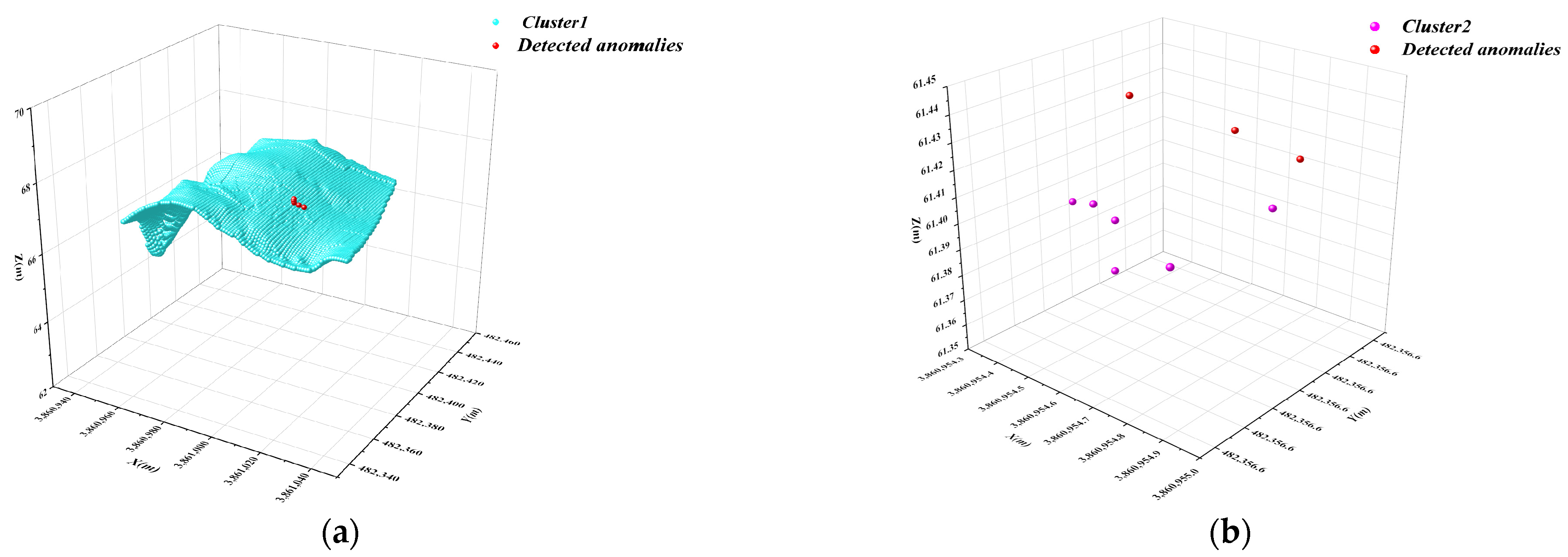
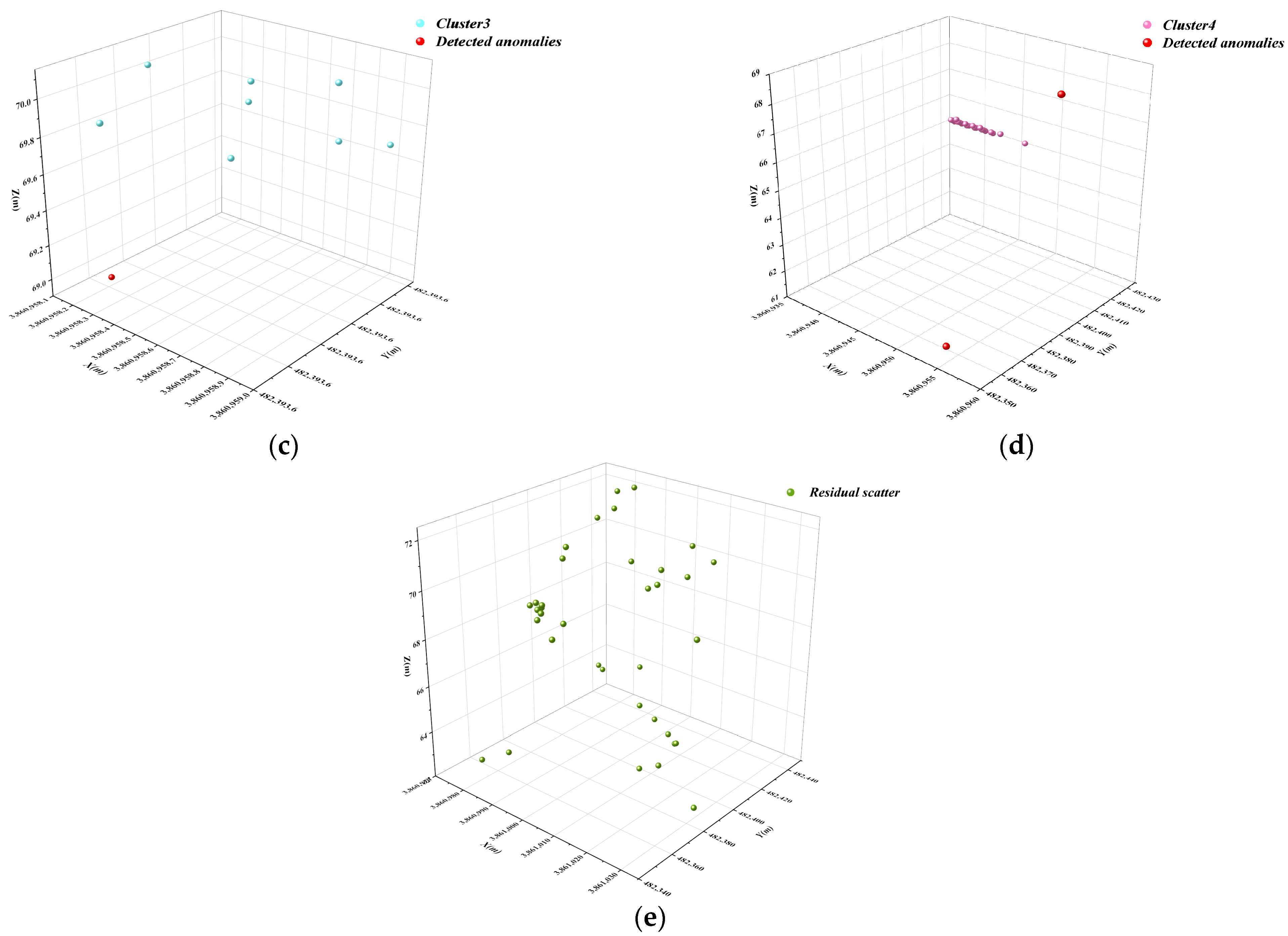
First-round screening by the DBSCAN algorithm. In the screening by this algorithm, the dataset is divided into numerous subclusters, and the values in each cluster that do not satisfy the screening conditions of the DBSCAN algorithm are marked as anomalies. After this calculation, the original dataset is divided into numerous subclusters, and local outliers in each cluster, which have fewer than Minpts neighbours within the radius, are identified.

(4)

Secondary detection by the IForest algorithm. Because the DBSCAN algorithm is unable to identify regional outliers with more than Minpts neighbours, the isolated forest algorithm is subsequently applied to the model to carry out secondary screening of the subclusters; this completes the step-by-step anomaly detection process, and the outliers obtained from these two steps of detection are combined to obtain the final results of anomaly detection.

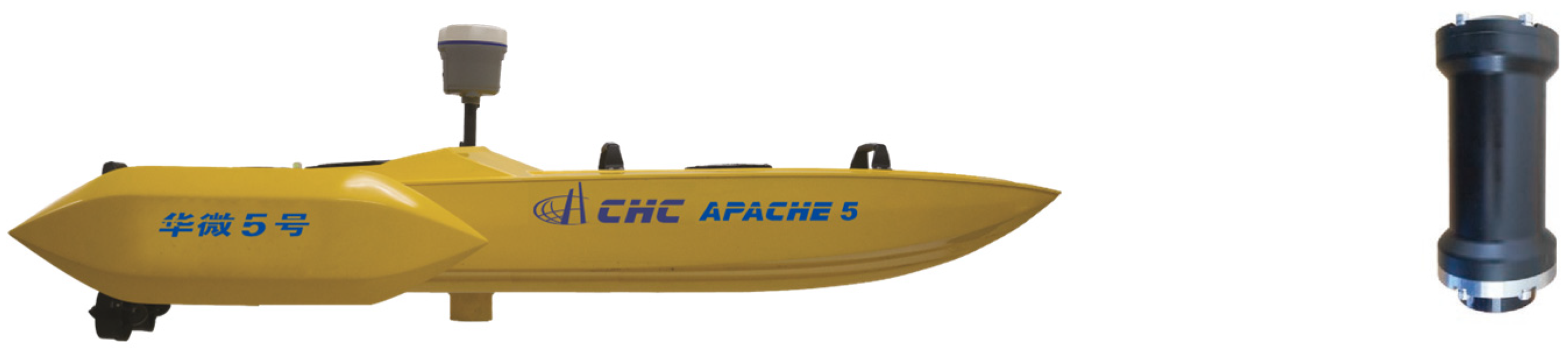
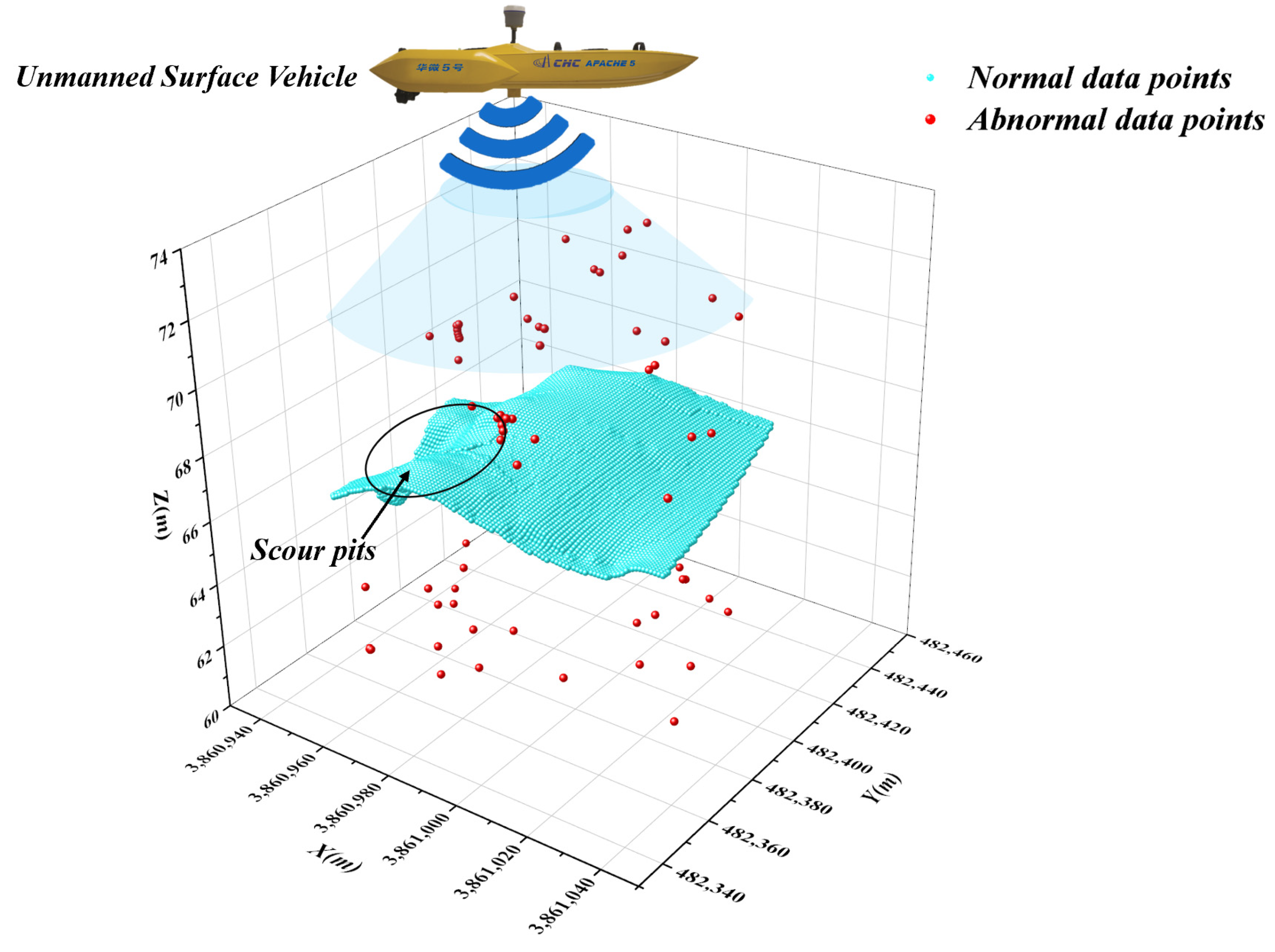
2.6. Data Acquisition

Underwater topographic data are acquired via an unmanned vessel equipped with a single-beam sounder (see Figure 4). The unmanned vessel is 1.6 m long and 0.38 m wide and has a working weight of 10.2 kg, with a single-beam sounder in the cabin, a Samsung eight-frequency GNSS receiver, and an ion thruster with a power of 500 W; the maximum speed of the vessel is 5 m/s [26]. The single-beam sounder is an HY1611 model, with an operating frequency of 446 kHz, and the measurement range can reach 50 m, with an accuracy of 1 cm ± 0.1% of the measured depth. The measurement rate is related to the range, with a maximum of 20 measurements/second. In addition, the data analysis was performed using Python (version 3.8) with the scikit-learn library.

All measurement instruments were calibrated before and after each data collection session using standard reference materials to ensure accuracy. Regular maintenance checks were performed to minimise instrumental drift and systematic errors.

On 9 September 2024, onsite measurements were carried out at the Madu Dangerous Project in the lower reaches of the Yellow River, as shown in Figure 5; this project is located in Zhengzhou City, Henan Province, and has a similar structure to that of the Ding Dam, which is a river improvement project in the Yellow River Basin. The area surrounding the Yellow River Madu Dangerous Project is geographically and geologically significant, located along the middle reaches of the Yellow River in the North China Plain. Geographically, the region features flat to gently rolling terrain formed by millennia of sediment deposition from the Yellow River, creating fertile soils ideal for agriculture but also a dynamic and ever-shifting river channel prone to meandering and flooding. Geologically, the area is underlain by thick Quaternary alluvial deposits of sand, silt, and clay, which are highly erodible and contribute to the river’s exceptionally high sediment load. This soft, loose sediment makes the region vulnerable to erosion, landslides, and frequent course changes, particularly during high-flow periods. The combination of flat geography and unstable geology underscores the necessity of engineering interventions like the Madu Dangerous Project to stabilise the riverbanks, mitigate flood risks, and protect the surrounding agricultural land and communities [27].

According to records from the Huayuankou hydrological station, the river flow rate on the day of measurement was 867 m³/s, with a flow velocity of 1.2 m/s, a water temperature of 12 °C, and a sediment concentration of 2 kg/m³, as shown in

Table 1. Summary table of river gauging conditions.

Entry	Description/Information
Date	9 September 2024
Location	Zhengzhou city
Discharge	867 m3/s
Sensor	Single-beam sounder
Sediment concentration	2 kg/m3
Flow rate	1.2 m/s
temperature of the body of water	12 °C

. Due to the limited battery life of the measurement device, the sensor sampling interval was set to 1 m and data were collected only once at a point interval of 1.0 m. As shown in Figure 6, the measurement results clearly indicated scouring and undulation of the submerged terrain, especially in the area close to the construction, where there were obvious scour pits. Owing to the high sediment content of the Yellow River channel and the complexity of underwater scouring and siltation, the sound waves emitted by the single-beam sounder during operation were scattered and absorbed by the sediment particles, resulting in a weakened reflection signal. In addition, the specific morphological patterns of the riverbed, such as scouring pits, river-centre beaches and other topographic features, triggered multipath reflection, and interference of the acoustic signals, which together led to anomalous points in the present measurement data, as shown by the red scattered dots labelled in Figure 6.

3. Results and Analyses

In this section, the proposed algorithm is validated by using real underwater topographic data from the Madu Dangerous Project in the lower reaches of the Yellow River obtained in the previous section. To ensure the comparability of the calculation results of different methods in later sections and to avoid the adverse effect of the wide range of misjudgements that may be generated by some algorithms, we define the evaluation index of the anomaly detection effect as the detection rate P:

$$\mathrm{P}={\displaystyle \frac{{\mathsf{\partial }}_{\mathit{d}}}{{\mathsf{\partial }}_{\mathit{a}}}}\times {\displaystyle \frac{{\mathrm{\beta }}_{\mathit{d}}}{{\mathrm{\beta }}_{\mathit{t}}}}$$

(4)

where ${\mathsf{\partial }}_{\mathit{d}}$ is the number of detected anomalies, ${\mathsf{\partial }}_{\mathit{a}}$ is the number of all anomalies, ${\mathrm{\beta }}_{\mathit{d}}$ is the number of detected anomalies, and ${\mathrm{\beta }}_{\mathit{t}}$ is the total number of detected anomalies (efficiency × accuracy rate).

3.1. Optimisation of the DBSCAN Algorithm Parameters

To accurately determine the neighbourhood radius ε, the K-distance plot method was used for the analysis. Given the frequency setting of the single-beam sounder used in this study and its data sampling characteristics in a three-dimensional measurement space, eight data points are uniformly distributed around most of the acquisition points, except for the measurement boundary points and anomalous noise points. Considering that anomalies usually behave as outliers within a small area, a k value of 9 was selected for the K-distance map calculation.

As shown in Figure 7, the calculation of the K-distance map yields the distribution of distances between the data points and their kth nearest neighbours. Since the sampling spacing of the single-beam sounder is fixed, the distance values of most of the data points in the plot are concentrated at approximately 1.9. However, at the 6834th point on the curve, the corresponding distance value suddenly increases to approximately 2.416 and then continues to increase to 7.76. According to the basic principle of the K-distance plot, the ε value is usually chosen at the point where the curve undergoes an abrupt change, i.e., the location where the data points shift from a dense to a sparse distribution. Therefore, the distance value of 2.416, corresponding to the 6834th point on the curve, was selected as the ε value. This result graphically indicates the inflection points in the distance distribution of the data points, thus providing a better balance between the compactness of the clusters and the ability to identify noisy points.

In determining the value of Minpts, an efficient calculation method based on the Kd-tree was used. First, for each point object in the original dataset, the number of neighbouring points N within a preset scanning radius ε was determined, and the number of neighbouring points with the highest frequency of occurrence within a given neighbourhood radius was selected as the Minpts value after frequency analysis was performed on these statistics. After the statistics were analysed, it was determined that when ε is set to 2.416, the number of neighbouring points with the highest frequency of occurrence within that neighbourhood radius is 5, so the Minpts value is set to 5.

3.2. Underwater Terrain Data Clustering and Primary Screening with DBSCAN

After determining the appropriate ε value and Minpts, the DBSCAN algorithm was used to screen the underwater terrain data by preliminary clustering, and the results are shown in Figure 8. After processing by this algorithm, all the data were effectively divided into five clusters. Clusters 1 to 4 were found to be more effective: cluster 1 mainly contains normally measured underwater terrain data points, which are closely and uniformly distributed, with only a few anomalous data points; clusters 2 to 4 are a mixture of normal data and anomalous data, which are somewhat dispersed in their respective ε-domains. In contrast, cluster 5 consists of the remaining points from the screening of the first four clusters; the density of data points within this cluster is low, and they lack significant clustering characteristics.

While splitting the clusters, the DBSCAN algorithm also performs preliminary identification of outliers in the data within clusters 1 through 4, which are clearly identified by red dots in the Figure 8. The results clearly show that the DBSCAN algorithm has strong preprocessing ability when dealing with high-dimensional data, and it is able to accurately partition the original data into different subclusters according to their spatial distribution characteristics on the basis of the preset ε-radius. However, given the inhomogeneity of the density distribution within the subclusters, the algorithm’s anomaly detection effect at the subcluster level is somewhat average.

3.3. Isolated Forest Algorithm for Secondary Anomaly Screening of Subcluster Data

On the basis of the data processing results in the previous section, the isolated forest algorithm was further utilised to implement secondary fine screening for each subcluster, the screened anomalies were counted, and the results are shown in Figure 9. After the second screening of the isolated forest algorithm, most of the anomalies are effectively detected. However, there are still a few anomalies that are not identified. After analysis, these missed anomalies have extremely similar horizontal and vertical coordinates and elevation data. In the first round of screening using the DBSCAN algorithm, the algorithm failed to identify this cluster of anomalies as an anomaly because it had a high density and the number of points within its ε radius exceeded the preset Minpts threshold. In the subsequent screening by isolated forest, despite the algorithm’s high sensitivity to global outliers, the density of the cluster of outliers still seemed relatively low compared with the overall density of the global data, with the result that the isolated forest algorithm also failed to identify these outliers.

4. Detection Effectiveness of Relevant Anomaly Detection Methods

This paper compares and analyses the effectiveness of various existing data detection methods, such as the box-and-line plot method, LOF algorithm, K-means algorithm, DBSCAN algorithm, spatial autocorrelation algorithm, autoencoder, and isolated forest algorithm, in recognising underwater topographic data and compares them with the proposed detection methods.

4.1. DBSCAN Algorithm

The basic principles of this algorithm were described in detail in the previous section, and

Table 2. Computational results of the DBSCAN algorithm.

ε Value	Minpts Value	Total Detected	Detection Rate P
0.5	[2, 11]	[6956, 6973]	[1.14%, 1.15%]
1	[2, 9]	[1962, 6973]	[1.14%, 4.07%]
1.5	[2, 9]	[61, 63]	[76.25%, 78.75%]
2	[2, 9]	[56, 60]	[70.00%, 75.00%]
3	[2, 25]	[38, 70]	[47.50%, 87.5%]
4	[2, 45]	[16, 44]	[20.00%, 55.00%]

lists the detection results for different combinations of ε and Minpts parameter values. The table shows that the algorithm performs well in identifying single-point outliers when ε and Minpts take appropriate values [15]. Specifically, under a fixed value of ε, if the number of detected anomalies does not change greatly with increasing Minpts, then the detection accuracy is usually high and stable. However, there are significant differences in the recognition results under different ε values. For example, when ε is set to 1 and the Minpts value is in the range of 2 to 9, the results of its screened outliers are basically the same. However, when the Minpts value exceeds 9, the algorithm incorrectly categorises all the data points as anomalies, which may be due to the sampling spacing characteristics of the underwater terrain data. Figure 10 shows the anomaly test results corresponding to ε = 3 and Minpts = 25.

4.2. Isolated Forest Algorithm

The principle of this method was thoroughly explained in a previous section. The figure below shows the specific results of anomaly detection performed by the algorithm. Figure 11 clearly shows that the algorithm performs well in identifying single-point outliers. However, when detecting regional population outliers, its recognition effect is relatively poor [28], which is mainly because, in the process of constructing the decision tree, the path lengths of neighbouring population scatter values tend to be similar, leading to the algorithm misjudging these population scatter values.

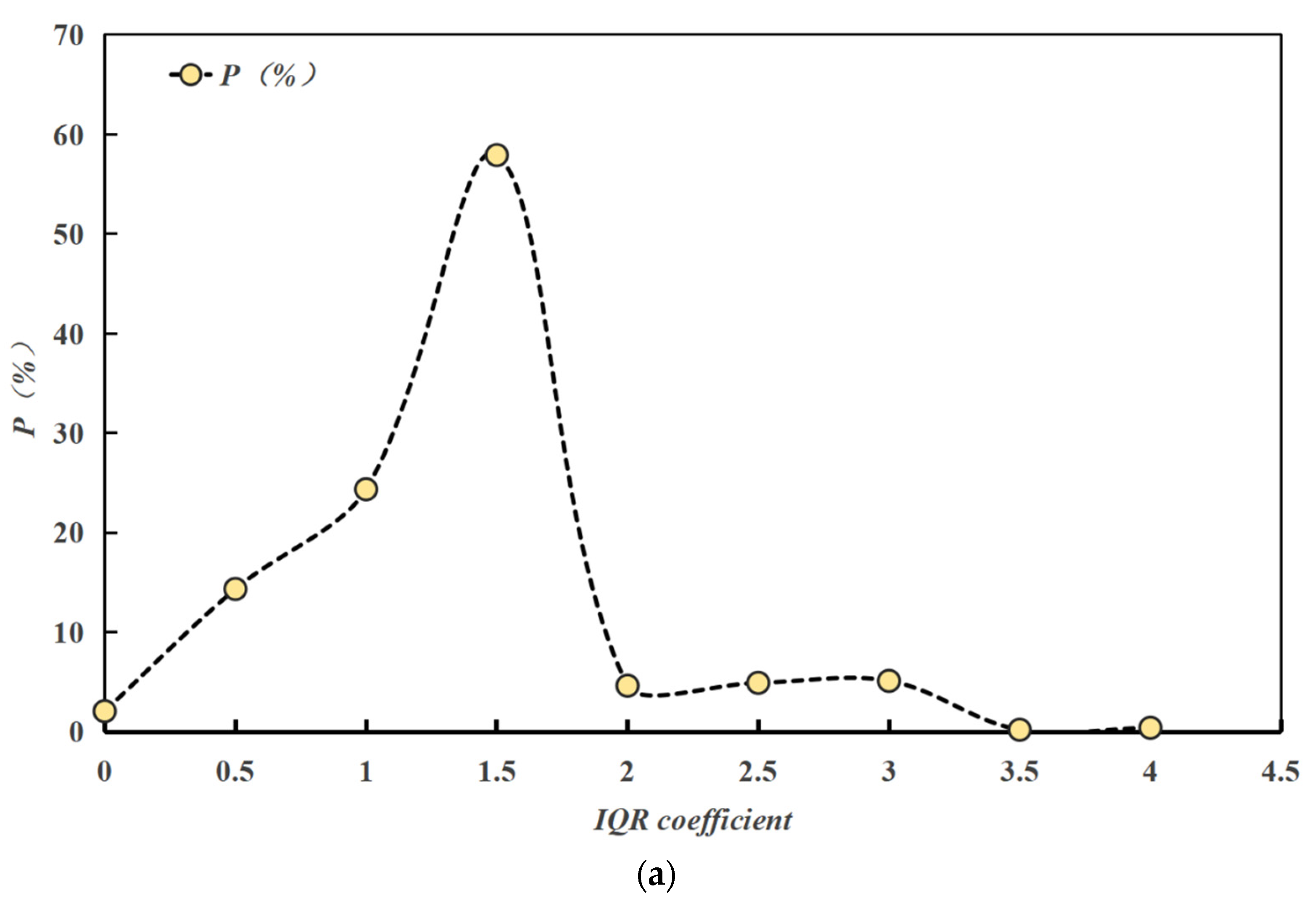
4.3. Box Plot Method

Boxplots are graphical tools for describing data distributions; they define the data range on the basis of the minimum, first quartile (Q1), median (Q2), third quartile (Q3), and maximum values, and they determine the boundaries of anomalous values on the basis of the interquartile spacing (IQR = Q3 − Q1) and the IQR coefficient, k. The upper and lower boundaries of anomalous values are determined by the formulae Q3 + k × IQR and Q1 − k × IQR. The IQR coefficients have a significant effect on the anomaly detection results, but in underwater topographic measurements, the setting of the IQR coefficients may lead to misjudgements due to unknown actual conditions.

Figure 12a shows the relationship between the p values obtained with different coefficients and the value of the IQR coefficient k. With increasing IQR coefficient k, p values refer to this evaluation metric, which was previously defined in the ’Results and analyses’ section, the value of P increases and then decreases, reaching a peak value of approximately 58% at k ≈ 1.5, as illustrated in Figure 12b, and then decreases sharply to nearly 0 at k = 3.5. Since the detection of anomalies relies on the summation of the boundary value and IQR, the detection effect is still acceptable when the summation value lies within the range of the measured value; beyond this range, the efficiency decreases sharply. In addition, the method identifies anomalies only from the perspective of the data distribution, which results in a high false positive rate.

4.4. LOF Algorithm

The LOF algorithm is a density-based anomaly detection method that identifies anomalies by comparing the local density of a target point with the density of other points in its neighbourhood [17]. This algorithm needs a preset value of k, i.e., a certain number of neighbourhood points are selected to characterise the local region, and the density is estimated using the reciprocal of the distances of the nearest neighbours. The local density $\mathrm{\rho }(\mathrm{X})$ of point X can be calculated using the following equation [28]:

$$\mathrm{\rho }(\mathrm{X})={\displaystyle \frac{1}{{\mathrm{N}}_{\mathrm{K}}}}{\displaystyle \sum _{\mathrm{i}=1}^{{\mathrm{N}}_{\mathrm{k}}}\frac{1}{\mathrm{d}({\mathrm{N}}_{\mathrm{i}},\mathrm{X})}}$$

(5)

Assume that the local densities of the k nearest neighbours of the point X are ${\mathrm{\rho }}_1$, ${\mathrm{\rho }}_2$,...,${\mathrm{\rho }}_{\mathrm{k}}$. For each neighbourhood point ${\mathrm{N}}_{\mathrm{i}}$, we calculate the distance d from its ${\mathrm{\rho }}_{\mathrm{i}}$ and ${\mathrm{N}}_{\mathrm{i}}$ to point X. The LOF value is calculated as follows [17]:

$$\mathrm{L}\mathrm{O}\mathrm{F}(\mathrm{X})={\displaystyle \frac{1}{\mathrm{k}}}{\displaystyle \sum _{\mathrm{i}=1}^{\mathrm{k}}\frac{{\mathrm{\rho }}_{\mathrm{i}}}{\mathrm{\rho }}}{\displaystyle \frac{1}{\mathrm{d}({\mathrm{N}}_{\mathrm{i}},\mathrm{X})}}$$

(6)

In general, points with LOF values much greater than 1 are considered anomalous because they are significantly less dense than other points in their neighbourhood [29].

Table 3. Computational results of the LOF algorithm.

K Value	Total Anomalies Detected	Number of Detected Anomalies	Detection Rate P
1	53	53	66.25%
2	71	71	88.75%
3	71	68	81.40%
4	142	68	40.70%
5	70	67	80.16%
6	71	65	74.38%
7	130	64	39.38%
8	183	63	27.11%
9	70	69	85.01%

shows the sensitivity analysis results of the LOF algorithm when performing anomaly detection. The setting of the k value of the number of initial neighbourhood points in the LOF algorithm has a significant effect on the detection results, but different k values may yield approximate results, considering that the distribution of anomalies may be uneven and that anomalies may be more concentrated in certain regions. As the k value increases, the detection accuracy initially tends to increase, but when the k value increases to a certain extent, the anomaly features may be masked by the neighbouring normal points, and the anomalous features will reappear under the scale of larger k values. The k value setting is closely related to the distribution of underwater topographic point data, which are often unknown, increasing the uncertainty of the k value setting and thus affecting the accuracy of detecting anomalous points. Figure 13 shows the anomaly detection results when k = 2.

4.5. K-Means Algorithm

The algorithm starts by randomly selecting k data points as the initial cluster centres and then performs the following iterative steps: first, the distance from each data point to each cluster centre is calculated and assigned to the nearest centre; then, each cluster centre is updated with the mean value of the data points of its members. This iterative process continues until the cluster centre position is stable or a preset number of iterations is reached. Ultimately, outliers can be identified on the basis of the distance from the data points to the cluster centre to which they belong, i.e., the points that are far from the cluster centre are considered outliers [30].

Figure 14 shows the computational results of this algorithm, from which it can be observed that several boundary points are misclassified as outliers. Given the three-dimensional nature of underwater terrain data, the algorithm uses the Euclidean distance as the distance between the points and the clustering centres. In the boundary region of the values, data points are prone to being incorrectly labelled as anomalies, as they may be far from all the selected clustering centres. In addition, the algorithm determines the distribution of anomalies only in terms of spatial distance; however, underwater topographic data are often subject to localised siltation and scouring, resulting in potentially small and sharp changes in the data distribution [31]. For this type of data, the algorithm may not be able to identify outliers accurately, and there is a risk of identification failure.

4.6. Spatial Autocorrelation Algorithm

The algorithm detects the distribution of similar values in geographic or spatial data and evaluates the distribution pattern of topographic data by constructing a spatial weight matrix and calculating spatial autocorrelation metrics such as Moran’s I and Geary’s C. The algorithm is also able to detect the distribution of similar values in geographic or spatial data. On the basis of these metrics, the algorithm is able to identify anomalies that do not match the surrounding features, i.e., points where the data values are significantly different from the surrounding values or overall trend [32].

Moran’s I is the most commonly used metric for measuring global spatial autocorrelation. Its formula is as follows [33]:

$$\mathrm{I}={\displaystyle \frac{\mathrm{N}}{\mathrm{W}}}{\displaystyle \frac{{\displaystyle {\sum }_{\mathrm{i}}{\displaystyle {\sum }_{\mathrm{j}}{\mathrm{\omega }}_{\mathrm{i}\mathrm{j}}({\mathrm{x}}_{\mathrm{i}}-\overline{\mathrm{x}})({\mathrm{x}}_{\mathrm{j}}-\overline{\mathrm{x}})}}}{{\displaystyle {\sum }_{\mathrm{i}}{({\mathrm{x}}_{\mathrm{i}}-\overline{\mathrm{x}})}^2}}}$$

(7)

where $\mathrm{N}$ is the total number of observations; ${\mathrm{x}}_{\mathrm{i}}$ and ${\mathrm{x}}_{\mathrm{j}}$ are the observations at positions i and j; $\overline{\mathrm{x}}$ is the average of the observations; ${\mathrm{\omega }}_{\mathrm{i}\mathrm{j}}$ is an element in the spatial weight matrix; E denotes the spatial relationship (e.g., the reciprocal of the distance) between positions i and j; and $\mathrm{W}$ is the sum of all ${\mathrm{\omega }}_{\mathrm{i}\mathrm{j}}$.

Moran’s I is in the range [−1,1], with positive values indicating positive autocorrelation, negative values indicating negative autocorrelation, and near-zero values indicating no autocorrelation. In positive autocorrelation, points higher than the mean value of neighbouring points may be abnormal; in negative autocorrelation, points lower than the mean value of neighbouring points may be abnormal.

Figure 15 shows the anomaly detection results of the algorithm. The regional anomalous point clusters are effectively identified, but most of the isolated anomalous scatter points are not detected. This is because Moran’s I metric focuses mainly on the overall spatial distribution trend of the data and is designed to determine whether there is global spatial autocorrelation of the data, i.e., whether the data values show a spatially clustered or dispersed pattern. However, as a global statistic, Moran’s I is less sensitive to local outliers, which may lead to some reduction in the ability to identify local outliers.

4.7. Autoencoder Algorithm

The autoencoder algorithm finds anomalies by learning data feature representations. It consists of an encoder and a decoder: the encoder maps the input to a low-dimensional space, and the decoder reconstructs the data. The reconstruction error reflects the input and output differences; a larger reconstruction error indicates that the decoder is unable to reconstruct the input data accurately and may contain anomalies. According to the 3-sigma principle, data points at which the reconstruction error exceeds the mean plus three times the standard deviation are considered anomalous [33].

The encoder maps the input data x to the hidden representation h [34], which can be expressed as $\mathrm{h}=\mathrm{f}\left({\mathrm{W}}_{\mathrm{e}}\cdot \mathrm{x}+{\mathrm{b}}_{\mathrm{e}}\right)$, where ${\mathrm{W}}_{\mathrm{e}}$ is the weight matrix of the encoder; ${\mathrm{b}}_{\mathrm{e}}$ is the bias vector; $\mathrm{f}$ is the activation function; the decoder maps the hidden representation h back to the original data space, i.e., reconstructs the input data; ${\mathrm{x}}^{\prime }=\mathrm{f}\left({\mathrm{W}}_{\mathrm{d}}\cdot \mathrm{h}+{\mathrm{b}}_{\mathrm{d}}\right)$, where ${\mathrm{W}}_{\mathrm{d}}$ are the weight matrices of the decoder and ${\mathrm{b}}_{\mathrm{d}}$ is the bias vector; and the error is usually represented by a squared loss function $\mathrm{E}={‖\mathrm{x}-{\mathrm{x}}^{\prime }‖}^2$.

Figure 16 shows the computational results of the algorithm, which misclassified more normal underwater terrain data than the other methods. This may be due to the extreme complexity and diversity of underwater terrain data, which cover a wide range of terrain features such as scour pits and siltation areas. The algorithm’s structure is relatively simple, containing only one encoder and decoder layer, which may not be sufficient to capture the complex patterns and features in the data, leading to errors in the model’s reconstruction of the complex terrain data and resulting in less satisfactory anomaly detection. In addition, the algorithm starts with the original dataset to learn the distribution of normal patterns, so it may learn the distribution pattern of anomalies and therefore reduce the detection effectiveness.

Figure 17 shows a comparison of the detection rates of different methods for underwater terrain anomaly data, and the LOF algorithm and DBSCAN are selected as yielding the optimal computational results in the testing stage [17]. The results show that the optimised DBSCAN-IForest algorithm has a detection rate of 93.75%, which is significantly better than those of the other algorithms. This finding indicates that the optimised DBSCAN-IForest algorithm has high applicability for the detection of underwater terrain anomaly data.

5. Conclusions

In this study, an optimised DBSCAN-IForest anomaly detection algorithm is proposed for detecting anomalies in underwater terrain data, and measured data from the Madu Dangerous Project on the Yellow River are selected for empirical analysis and verification. By systematically comparing the proposed algorithms with many commonly used algorithms and analysing the results, the developed algorithm is shown to have excellent performance in terms of accuracy and displays significant advantages over existing algorithms. The main conclusions are summarised as follows.

(1)

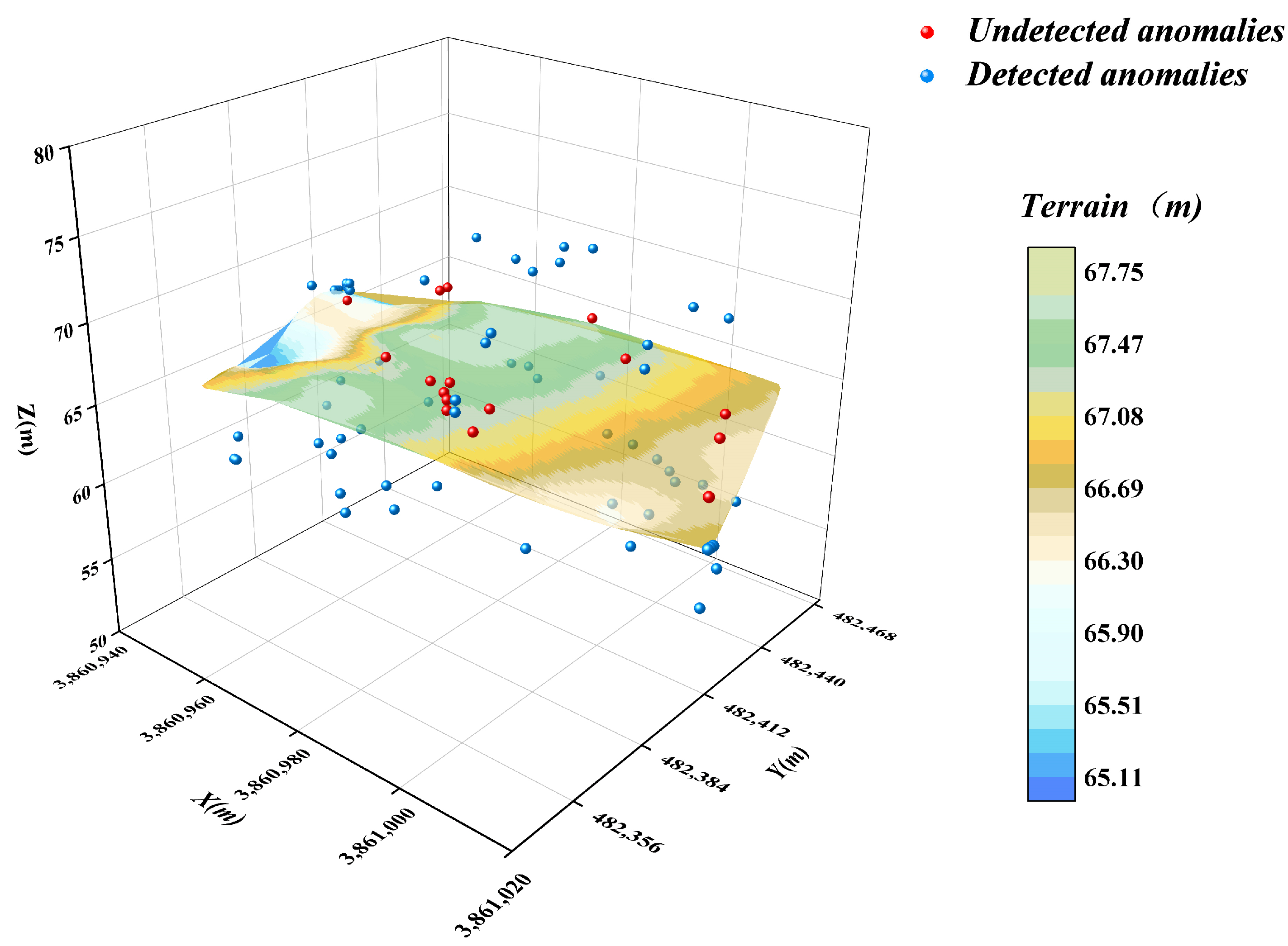
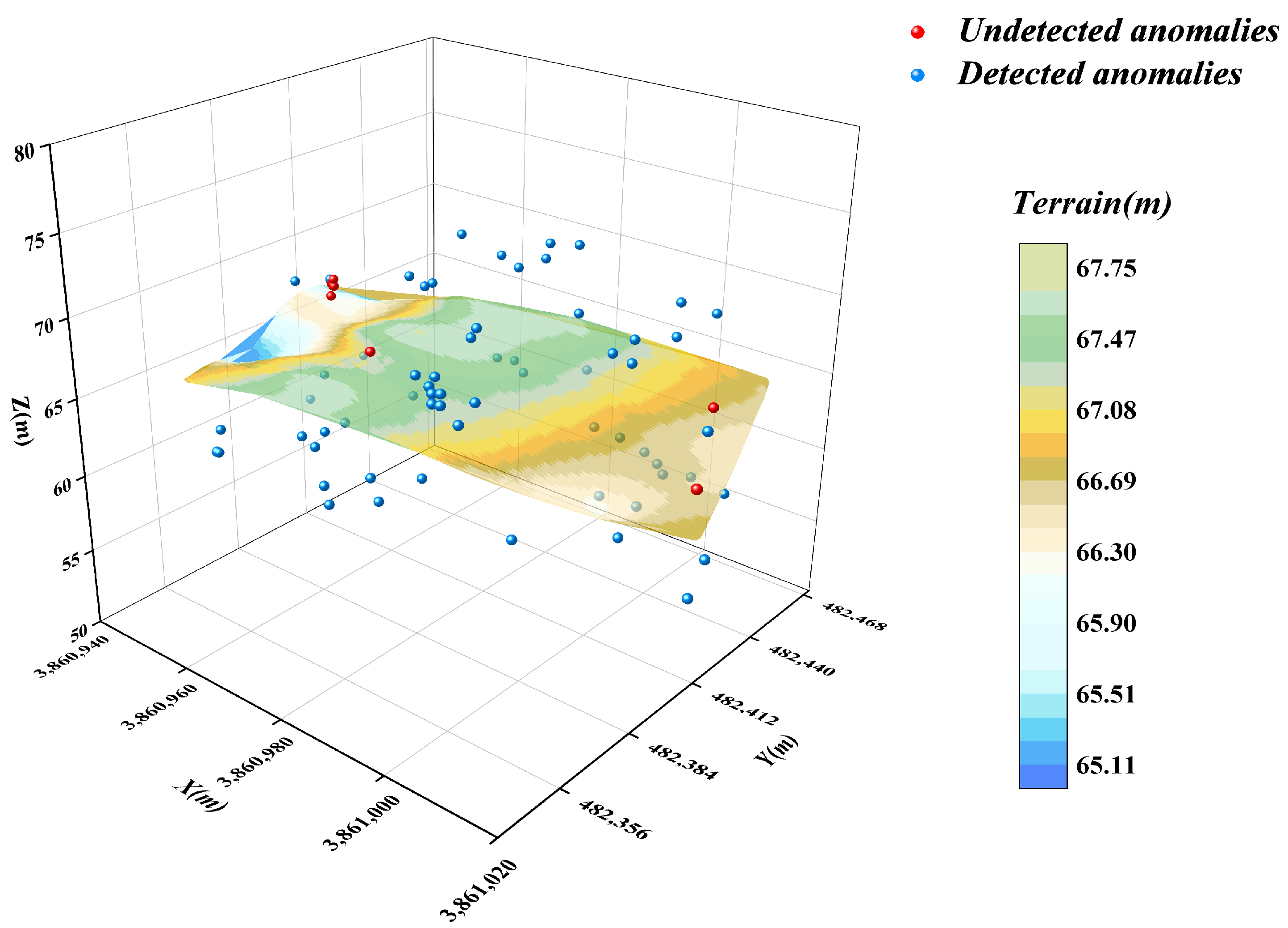
In this paper, an optimised DBSCAN-IForest stepwise anomaly detection algorithm is proposed, which integrates the K-distance map and Kd-tree techniques to accurately determine the ε and Minpts parameters in the DBSCAN algorithm; the algorithm follows step-by-step processing, in which the DBSCAN algorithm is used to initially screen the underwater terrain data in clusters. The isolated forest algorithm is subsequently introduced to perform more detailed outlier detection on the preliminary subclusters. The results show that the detection rate of the algorithm reaches 93.75%, higher than those of the other detection methods, which demonstrates the significant superiority of the algorithm.

(2)

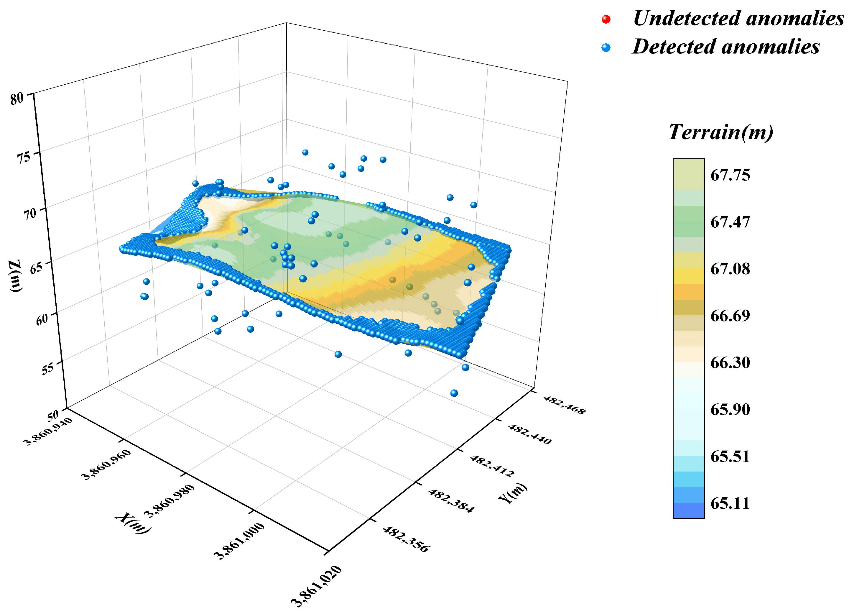
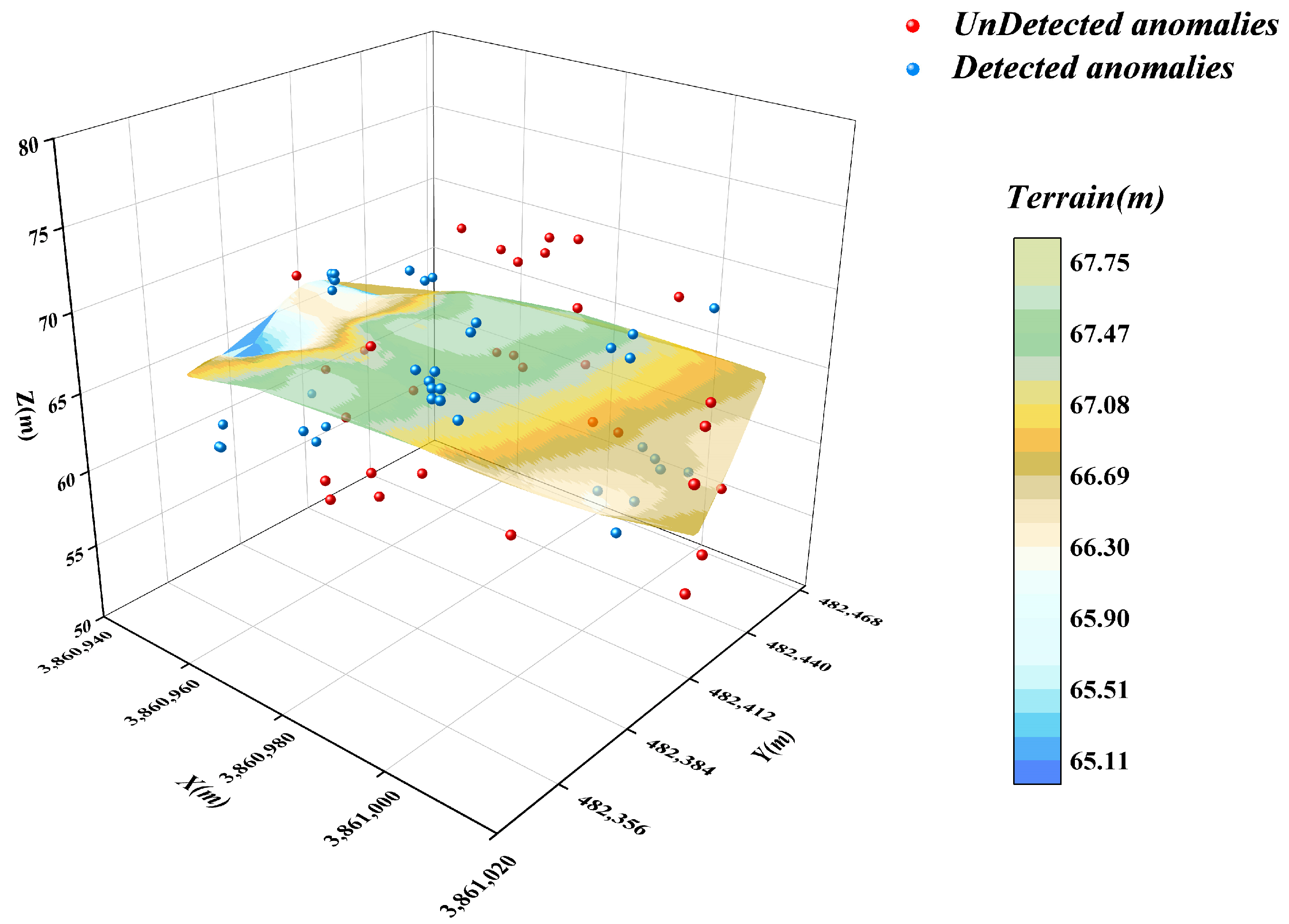
The effectiveness of commonly used anomalous data detection methods is verified by examples. Among these methods, the DBSCAN algorithm is based on the principle of density reachability, and its anomaly detection results are sensitive to the setting of the neighbourhood radius ε and the minimum number of points Minpts, this may affect the stability of the results. The isolated forest algorithm identifies anomalies by measuring the degree of isolation of the data points in the feature space; it is effective in identifying the outliers at a single point but performs poorly in addressing regional anomalies. The box-and-line diagram method is based on the characteristics of the data distribution. It is easy to perform, but the accuracy is easily affected by the IQR coefficients. The LOF algorithm identifies anomalies by comparing local densities, but its results are significantly dependent on the selection of the value k of the number of initial neighbourhood points. K-means is prone to misjudging the data in the boundary region. In addition, the spatial autocorrelation algorithm has a limited ability to detect local anomalies. The autoencoder identifies anomalies by learning the feature representation of the data, but its detection effect is average in the case of complex and diverse underwater terrain data.

(3)

The optimised DBSCAN-IForest algorithm proposed in this study has good applicability in underwater subsurface data detection, and the research results not only provide valuable reference data for anomalous data detection in other fields but also help improve hydrological measurement technology to reach a higher level of scientific and automated development. However, this study has certain limitations. Firstly, the sample size of the dataset used for analysis is limited, which may affect the generalizability of the results to broader or more diverse underwater environments. Secondly, variations in data collection conditions, such as changes in underwater topography, equipment performance, and environmental factors, could introduce uncertainties into the detection process.

References

1. Wang, H. Research on the Theory and Method of Processing Anomalies in Bathymetry of Multibeam System. Ph.D. Thesis, PLA Information Engineering University, Zhengzhou, China, 2012. (In Chinese). [Google Scholar]
2. Cheng, X. Research on Key Technology of Multibeam Measurement Data Processing. Master’s Thesis, Shandong University of Architecture, Jinan, China, 2014. (In Chinese). [Google Scholar]
3. Huang, S.Q.; You, H.; Wang, Y.T. Environmental monitoring ofnatural disasters using synthetic aperture radar image multi-directional characteristics. Int. J. Remote Sens. 2015, 36, 3160–3183. [Google Scholar] [CrossRef]
4. Huang, J.; Zhang, Y.; Ding, J. Combining LiDAR, SAR, and DEM Data for Estimating Understory Terrain Using Machine Learning-Based Methods. Forests 2024, 15, 1992. [Google Scholar] [CrossRef]
5. Cao, D.; Wang, C.; Du, M.; Xi, X. A Multiscale Filtering Method for Airborne LiDAR Data Using Modified 3D Alpha Shape. Remote Sens. 2024, 16, 1443. [Google Scholar] [CrossRef]
6. Blaszczak-Bak, W.; Birylo, M. Study of the Impact of Landforms on the Groundwater Level Based on the Integration of Airborne Laser Scanning and Hydrological Data. Remote Sens. 2024, 16, 3102. [Google Scholar] [CrossRef]
7. Liu, F.T.; Ting, K.M.; Zhou, Z.-H. Isolation-Based Anomaly Detection. ACM Trans. Knowl. Discov. Data 2012, 6, 1–39. [Google Scholar] [CrossRef]
8. Cui, X.; Chang, B.; Zhang, S.; He, J.; Zhi, Z.; Zhang, W. Anomaly Detection in Multibeam Bathymetric Point Clouds Integrating Prior Constraints with Geostatistical Prediction. IEEE J. Sel. Top. Appl. Earth Obs. Remote Sens. 2024, 17, 17903–17916. [Google Scholar] [CrossRef]
9. Zhou, P.; Chen, J.; Wang, S. A Dual Robust Strategy for Removing Outliers in Multi-Beam Sounding to Improve Seabed Terrain Quality Estimation. Sensors 2024, 24, 1476. [Google Scholar] [CrossRef] [PubMed]
10. Yoshimura, N.; Kuzuno, H.; Shiraishi, Y.; Morii, M. DOC-IDS: A Deep Learning-Based Method for Feature Extraction and Anomaly Detection in Network Traffic. Sensors 2022, 22, 4405. [Google Scholar] [CrossRef] [PubMed]
11. Nicholaus, I.T.; Park, J.R.; Jung, K.; Lee, J.S.; Kang, D.-K. Anomaly Detection of Water Level Using Deep Autoencoder. Sensors 2021, 21, 6679. [Google Scholar] [CrossRef]
12. Hu, G.; Zhou, X. Detection of Bathymetric Data Outliers in Ocean Surveying and Mapping. In Compilation of Papers on Ocean Development and Sustainable Development in the 14th Session of the 2004 Academic Annual Meeting of the Chinese Association for Science and Technology; Chinese Society of Surveying and Mapping: Beijing, China, 2004; p. 6. (In Chinese) [Google Scholar]
13. Zhang, R.; Bian, S.; Liu, Y.; Li, H. Conditional Variation Self-Coding Algorithm for Large-Area Bathymetric Anomaly Detection. J. Surv. Mapp. 2019, 48, 1182–1189. (In Chinese) [Google Scholar]
14. Long, J.; Zhang, H.; Zhao, J. A Comprehensive Deep Learning-Based Outlier Removal Method for Multibeam Bathymetric Point Cloud. IEEE Trans. Geosci. Remote Sens. 2023, 61, 1–22. [Google Scholar] [CrossRef]
15. Huang, X.; Huang, C.; Zhai, G.; Lu, X.; Xiao, G.; Sui, L.; Deng, K. Data Processing Method of Multibeam Bathymetry Based on Sparse Weighted LS-SVM Machine Algorithm. IEEE J. Ocean. Eng. 2020, 45, 1538–1551. [Google Scholar] [CrossRef]
16. Li, H.; Ye, W.; Liu, J.; Tan, W.; Pirasteh, S.; Fatholahi, S.N.; Li, J. High-Resolution Terrain Modeling Using Airborne LiDAR Data with Transfer Learning. Remote Sens. 2021, 13, 3448. [Google Scholar] [CrossRef]
17. Breunig, M.M.; Kriegel, H.-P.; Ng, R.T.; Sander, J. LOF: Identifying Density-Based Local Outliers. ACM Sigmod. Rec. 2000, 29, 93–104. [Google Scholar] [CrossRef]
18. Abdelazeem, M.; Abazeed, A.; Kamal, H.A.; Mohamed, M.O.A. Towards an Accurate Real-Time Digital Elevation Model Using Various GNSS Techniques. Sensors 2024, 24, 8147. [Google Scholar] [CrossRef]
19. Bozzano, M.; Varni, F.; De Martino, M.; Quarati, A.; Tambroni, N.; Federici, B. An Integrated Approach to Riverbed Morphodynamic Modeling Using Remote Sensing Data. J. Mar. Sci. Eng. 2024, 12, 2055. [Google Scholar] [CrossRef]
20. Chen, P.; Li, Z.; Liu, G.; Wang, Z.; Chen, J.; Shi, S.; Shen, J.; Li, L. Underwater Terrain Matching Method Based on Pulse-Coupled Neural Network for Unmanned Underwater Vehicles. J. Mar. Sci. Eng. 2024, 12, 458. [Google Scholar] [CrossRef]
21. Hu, X.; Gao, Y.; Liu, K.; Xiang, L.; Luo, B.; Li, L. Surface Electromyographic Responses During Rest on Mattresses with Different Firmness Levels in Adults with Normal BMI. Sensors 2024, 25, 14. [Google Scholar] [CrossRef] [PubMed]
22. Zhou, S.; Zhou, A.; Cao, J. DBSCAN Algorithm Based on Data Partitioning. Comput. Res. Dev. 2000, 37, 1153–1159. (In Chinese) [Google Scholar]
23. Xiong, Z.; Zhu, D.; Liu, D.; He, S.; Zhao, L. Anomaly Detection of Metallurgical Energy Data Based on iForest-AE. Appl. Sci. 2022, 12, 9977. [Google Scholar] [CrossRef]
24. Li, X.; Gao, X.; Yan, B.; Chen, C.; Chen, B.; Li, J.; Xu, J. An Approach of Data Anomaly Detection in Power Dispatching Streaming Data Based on Isolation Forest Algorithm. Power Syst. Technol. 2019, 43, 1447–1456. (In Chinese) [Google Scholar]
25. Liu, W.; Mu, X.; Huang, Y. Anomaly Detection Method Based on Multi-Resolution Grid. Comput. Eng. Appl. 2020, 56, 78–85. (In Chinese) [Google Scholar]
26. Qi, C.; He, W.; Jiao, Y.; Ma, Y.; Cai, W.; Ren, S. Survey on Anomaly Detection Algorithms for Unmanned Aerial Vehicle Flight Data. J. Comput. Appl. 2023, 43, 1833–1841. (In Chinese) [Google Scholar]
27. Whitehurst, D.; Joshi, K.; Kochersberger, K.; Weeks, J. Post-Flood Analysis for Damage and Restoration Assessment Using Drone Imagery. Remote Sens. 2022, 14, 4952. [Google Scholar] [CrossRef]
28. Chen, P.; Seo, D.; Maity, B.; Dutt, N. KDTree-SOM: Self-Organizing Map Based Anomaly Detection for Lightweight Autonomous Embedded Systems. In Proceedings of the Great Lakes Symposium on VLSI 2024, Clearwater, FL, USA, 12–14 June 2024. [Google Scholar]
29. Zhao, J.; Yang, L. The Improvement and Implementation of DBSCAN Clustering Algorithm. Microelectron. Comput. 2009, 26, 189–192. (In Chinese) [Google Scholar]
30. Zhu, C.; Huang, P.; Li, L. Generalized Isolation Forest Anomaly Detection Algorithm Based on Expert Feedback. Appl. Res. Comput. 2024, 41, 88–93. (In Chinese) [Google Scholar]
31. Qiao, T.; Tong, D.; Wang, J.; Guan, T.; Wu, B. Outlier Detection and Correction for Rolling Speed Based on Kmeans-EMD and IWOA-Elman. J. Water Resour. Water Eng. 2022, 33, 124–131. (In Chinese) [Google Scholar]
32. Wang, X.; Bai, Y. The Global Minmax k-Means Algorithm. SpringerPlus 2016, 5, 1665. [Google Scholar] [CrossRef] [PubMed]
33. Deng, T.; Huang, Y.; Gu, J. Diagnosis of Spatial Autocorrelation in Spatial Analysis. Chin. J. Health Stat. 2013, 30, 343–346. (In Chinese) [Google Scholar]
34. Lai, J.; Wang, X.; Xiang, Q.; Song, Y.; Quan, W. Review on Autoencoder and Its Application. J. Commun. 2021, 42, 1–15. (In Chinese) [Google Scholar]
Figure 1. Computational principles of the DBSCAN algorithm.
Water 17 00626 g001
Figure 2. Computational framework for the isolated forest algorithm.
Water 17 00626 g002
Figure 3. Optimised DBSCAN-IForest algorithm implementation. (a) Calculation of spatial distances of topographic data points, (b) parameter calculation, and (c) Step-by-step anomaly detection.
Water 17 00626 g003
Figure 4. Unmanned vessels and sensors for underwater subsurface data measurements.
Water 17 00626 g004
Figure 5. Map of the study area. (a) Location of the survey area in Henan Province, (b) the Yellow River Channel, and (c) the Yellow River Madu Dangerous Project (Red circles mark specific project locations).
Water 17 00626 g005
Figure 6. Underwater topographic survey results.
Water 17 00626 g006
Figure 7. K-distance chart calculation results.
Water 17 00626 g007
Figure 8. Plot of the clustering and initial screening results of the DBSCAN algorithm ((ae) show the 5 subclusters in order).
Water 17 00626 g008aWater 17 00626 g008b
Figure 9. Optimised DBSCAN-IForest calculation results.
Water 17 00626 g009
Figure 10. Plot of results calculated by the DBSCAN algorithm (the graph shows the results corresponding to a detection rate of 87.5%).
Water 17 00626 g010
Figure 11. Results calculated by the isolated forest algorithm.
Water 17 00626 g011
Figure 12. Calculation results of the Box Plot. (a) Detection rate P versus IQR coefficient, (b) plot of results calculated by the Box Plot (the graph shows the results corresponding to a detection rate of 58%).
Water 17 00626 g012aWater 17 00626 g012b
Figure 13. Plot of the results calculated by the LOF algorithm (the figure shows the results corresponding to a detection rate of 88.75%).
Water 17 00626 g013
Figure 14. Plot of the results calculated by the K-means method.
Water 17 00626 g014
Figure 15. Plot of the results calculated by the spatial autocorrelation algorithm.
Water 17 00626 g015
Figure 16. Plot of the results calculated by the autoencoder.
Water 17 00626 g016
Figure 17. Comparison of the detection rates of various algorithms.
Water 17 00626 g017