Sensitivity Analysis-Aided Calibration of Urban Drainage Modeling

Abstract

This paper presents a novel methodology for the event-based calibration of urban drainage models based on conceptual simulation of external sub-catchments and physical representation of underground channels. Following the setup of the numerical model of an urban drainage system and the definition of the list of parameters, the methodology proposed is based on two steps, namely the application of sensitivity analysis for the identification of influent parameters and the calibration of the model on each event considering the reduced set of influent parameters by means of an optimizer. The methodology is applied to the Cascina Scala urban catchment in Pavia, northern Italy, for which a rainfall/runoff dataset is available for 14 events. In the applications, the urban drainage system is constructed in the EPA-SWMM environment, and a genetic algorithm is used for calibration. The results prove that the model parameterized with the innovative methodology features a very good fit to experimental data concerning hydrographs at the exit of the catchment while offering significant computational advantages compared with the usual calibration approach.

1. Introduction

By increasing the urbanization rate and the effects of climate change, the patterns of the hydrological cycle undergo changes [1,2,3,4]. These changes may put more pressure on the urban sewer systems by increasing runoff volume and inducing flash floods and water quality deterioration [5]. Accordingly, urban catchment analysis has become a critical aspect of sustainable water resource management, and accurate modeling of rainfall-runoff transformation is imperative for efficient drainage system design and definition of flood risk/hazard maps [6] and, thus, flood mitigation strategies. On the other hand, rainfall-runoff transformation constitutes a complex hydrological process involving several physical phenomena (i.e., precipitation, interception, infiltration, evapotranspiration, runoff [7]) depending on several parameters.

In the last decades, numerous hydrological models have been developed to simulate rainfall-runoff transformation in urban catchments. In this regard, one of the most widely used models, because of the model’s simple structure, open-source feature, and capability to consider several site-specific parameters (for both basins and drainage networks), is the Storm Water Management Model (SWMM) [8] of the United States Environmental Protection Agency [9]. It is a flexible tool designed to simulate both the quantitative and qualitative aspects of an urban drainage system, such as flow rates and volumes or pollutant concentrations and water quality parameters, respectively [5,7]. The advantage of this model is the capability of detailed hydrological modeling of the rainfall-runoff processes in a catchment, considering land uses, surface characteristics, and infiltration, among other aspects. In addition, it couples these hydrological processes with hydraulic modeling, enabling the simulation of water flows in pipe networks, open channels, and other drainage networks. This can make SWMM particularly effective in designing and managing stormwater systems, assessing flood risks, and evaluating impacts of various land use or climate scenarios on urban water infrastructure.

Moreover, EPA-SWMM is a semi-distributed model that allows sub-dividing the catchment into multiple sub-catchments by considering the specific characteristics of all of them. Although this represents a great advantage and is helpful for better understanding and modeling hydrological processes, it makes accurate model calibration mandatory, which may represent a challenging task [5].

In this regard, the model reliability depends on how the parameters are defined [10,11] and then, on the availability of high-quality rainfall-runoff measured data in order to find the optimal parameter values that maximize the fit of the model to experimental observation.

In recent years, automatic calibration methods have been widely developed for obtaining reliable estimations of the hydrological model’s parameter values [12,13,14], and the population-based heuristic Genetic Algorithm (GA) [15] is one of the most efficient optimization methods [16,17].

Generally, the calibration process can become cumbersome and computationally expensive due to the high number of parameters to be optimized. On the other hand, it is often unnecessary to consider all the model parameters for the calibration to achieve efficient optimization [18], and accordingly, it becomes useful to define a priori ineffective inputs through a sensitivity analysis (SA) and set them to fixed values. By identifying parameters that have a significant impact on the model output, SA helps in carrying model calibration, understanding the modeled system [19], and focused planning of further research and field measurement [20].

SA methods are generally classified as local or global [21]. Local SA can easily perform, interpret, and evaluate the local response of a model by individually varying input parameters while keeping all the others at a reference value. Even if such an approach does not consider possible nonlinear interactions between different parameters [22], as is with a global sensitivity analysis [23], its results are still very informative since the impact of input parameters on model outputs can be quantified through indices and then ranked. Furthermore, global sensitivity analysis generally requires a much higher number of simulations to obtain reliable results [24], and it may be computationally costly for complex models with many parameters.

Therefore, to improve the understanding of the hydrological response and the optimization of urban drainage modelling, an automatic sensitivity analysis-aided calibration of mostly impacting runoff parameters is proposed in this work for different registered rainfall events by linking EPA-SWMM 5.1 software to MATLAB^® R2023b. The methodology is applied to a real urban catchment of northern Italy, in Pavia. In this regard, this research aims to (1) quantify the importance of input parameters on the urban catchment behavior in terms of peak discharge and total volume of the hydrograph at the outlet section; (2) make the calibration step more efficient by optimizing only the most important parameters; (3) investigate the possible variability of the relative importance of the model parameters to the rainfall characteristics; and (4) compare the calibration performance of the modeling approaches with and without the preliminary sensitivity analysis step.

2. Materials and Methods

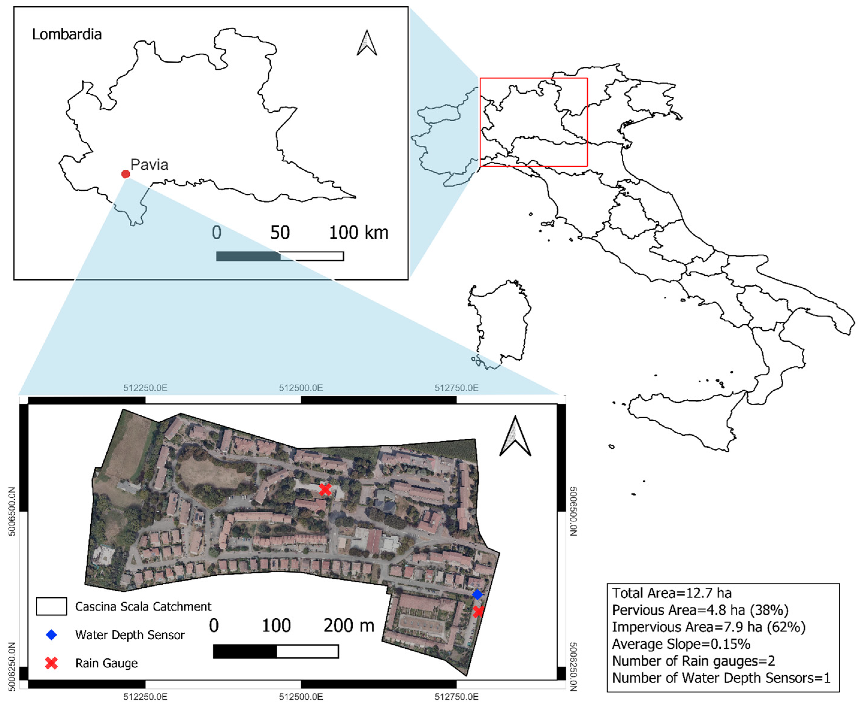
2.1. Case Study

The Cascina Scala urban catchment (Figure 1), located on the northern side of Pavia (Lombardia, Italy), was chosen as a case study. The catchment hosts about 1500 inhabitants, and the runoff contribution area is 12.7 ha, where 7.9 ha (62%) is impervious, and 4.8 ha (38%) is pervious [5,7,25,26].

The impervious area consists of 2.88 ha (22.0%) of roofs and 5.02 (39.6%) of streets and paved areas. The area has an average slope of 0.15%, and it is directly connected to the underground channels of the sewer system made up of 42 roughly 60-year-old concrete pipes, with an average slope of 0.42% and a total length of 2045 m. Notably, the upstream channels are circular conduits (diameter ranging between 0.4 m and 0.6 m), while the downstream channels are egg-shaped conduits (main sizes ranging between 0.6–0.9 m and 0.7–1.05 m).

The area can be divided into 42 sub-catchments, so each pipe drains the runoff from each sub-catchment. The main characteristics of each sub-catchment are listed in

Table 1. Cascina Scala sub-catchment characteristics.

ID	Area (ha)	Slope (%)	Impervious Area		ID	Area (ha)	Slope (%)	Impervious Area
			Roofs (%)	Streets (%)				Roofs (%)	Streets (%)
1	0.27	0.5	0	29.2	22	0.50	0.5	20.4	56.3
2	0.20	0.2	21.2	54.8	23	0.13	0.1	0	85.9
3	0.39	0.1	23.1	40.7	24	0.81	0.1	23.5	47.8
4	0.28	0.1	32.8	54.4	25	0.41	0.2	24.2	31.9
5	0.07	0.1	0	100	26	0.13	0.1	0	100
6	0.49	0.1	32.5	40	27	0.39	0.1	22.1	26
7	0.09	0.1	0	100	28	0.21	0.1	37.9	9
8	0.16	0.1	32.4	33.2	29	0.20	0.1	0	77.9
9	0.07	0.1	24.5	43.2	30	0.06	0.1	0	75.4
10	0.57	0.1	5.1	35.6	31	0.10	0.1	0	80.8
11	0.12	0.1	12.4	62.7	32	0.50	0.1	37.6	21.9
12	0.36	0.3	30.8	30.5	33	0.05	0.2	19.5	80.5
13	0.20	0.3	31.3	46.8	34	0.33	0.1	23.1	40.2
14	0.16	0.1	20.3	53	35	0.42	0.1	32	41.5
15	1.35	0.1	26.3	25.6	36	0.27	0.1	16	40.7
16	0.21	0.1	29.3	37.1	37	0.24	0.1	16.3	65.7
17	0.11	0.1	23.9	43.4	38	0.16	0.2	14.4	51.9
18	0.06	0.3	0	100	39	0.05	0.1	0	48
19	0.05	0.1	30.6	54.03	40	0.19	0.6	29.6	43.9
20	0.17	0.1	26.2	42	41	0.12	0.3	25.2	49.6
21	0.47	0.1	26.5	29.3	42	0.22	0.3	26.8	57.3
					42 *	1.55	0.3	25.1	21.1

Note(s): “*” indicates the modified catchment ID 42 after May 2001.

. From May 2001, an additional area of 1.33 ha was connected to the sewer system (to the sub-catchment ID 42), leading to an increase of the corresponding area from 0.22 ha to 1.55 ha (in Table 1, sub-catchment ID 42*).

Rainfall intensity and runoff measurements (at every minute) were carried out using two rain gauges (±2% precision and 0.2 mm resolution) and an ultrasonic water depth sensor (±2% precision), respectively (see Figure 1 for their positions). The distance between the two rain gauges is 310 m, and the second rain gauge is used to control rainfall homogeneity and assess rainfall volume better.

For the purposes of the current study, fourteen rainfall events, for which simultaneous measurements of rainfall intensity and flow rate were available, were selected for rainfall-runoff simulations.

Table 2. Main characteristics of selected rainfall events.

Event	Rainfall Duration (min)	Total Rainfall Depth (mm)	Peak Discharge (L/s)	Average Rainfall Intensity (mm/h)
3	196	11.84	247.1	3.62
5	109	16.39	551.0	9.02
7	50	6.99	325.5	8.39
8	64	10.99	375.9	10.30
9	215	10.61	161.5	2.96
11	478	26.21	280.7	3.29
12	443	18.62	262.8	2.52
13	110	8.39	157.3	4.57
14	380	15.80	256.7	2.50
17	964	23.40	128.2	1.46
19	248	12.56	231.9	3.04
20	231	16.22	212.0	4.21
21	445	8.57	61.3	1.16
23	1131	39.78	147.7	2.11

reports the main characteristics of these events, which meet the following conditions:

• No measurement device malfunctioning.
• No pressurized flow conditions.
• Rainfall depth equal to or greater than 5 mm.
• Maximum rainfall intensity equal to or greater than 0.1 mm/min.
• Maximum rainfall depth of at least 2 mm over 15 min.

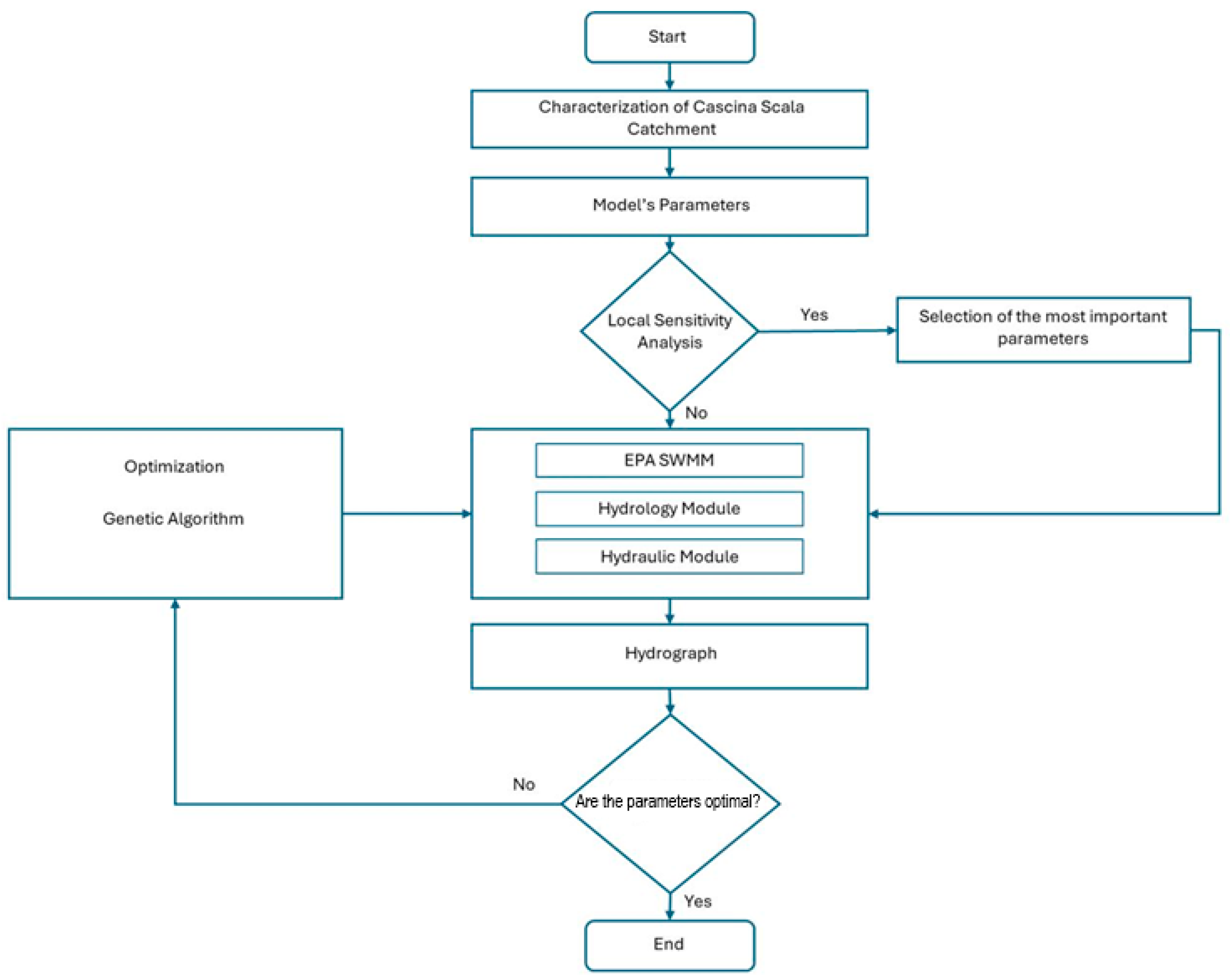
2.2. Methodology

The semi-distributed modeling approach was employed to simulate the rainfall-runoff transformation. In this regard, the EPA Storm Water Management Model (SWMM) [27] was adopted, which allows short- and long-term simulations for both water quantity and quality. Considering precipitation patterns as input, each sub-catchment is modeled as a nonlinear reservoir, for which surface runoff and infiltration are outputs, while evapotranspiration is neglected due to the short duration of the simulated phenomena. This aspect, along with the fact that vegetation is not considered, as well as more complex phenomena related to weather, allows disregarding feedback processes. The following sections detail the main steps of this study (see the flowchart in Figure 2).

2.2.1. Model Setup

For the nonlinear reservoir model, water storage is defined by the balance of inflow (precipitation) and outflow (infiltration, evaporation, and runoff) [5,26,27]. During the generic rainfall event, it begins to fill in, and the runoff starts only when the storage depth dominates the depression storage depth (which stands for surface wetting, interception, and ponding). The main equations that rule the rainfall-runoff transformation are listed in the following:

$${\displaystyle \frac{dD}{dt}}=i-f-r$$

(1)

Equation (1) represents the mass conservation for each sub-catchment, according to which the net change in water depth (D), at each time step (t), is the difference between inflow and outflow. Notably, $i$ is the rainfall intensity (m/s), $f$ is the infiltration rate (m/s), and $r$ is the runoff rate per unit of surface area (m/s).

By using Manning’s equation and assuming a uniform flow over sub-catchment, r can be computed through Equation (2):

$$r={\displaystyle \frac{W{\left(D-D_p\right)}^{\frac{5}{3}}{s}^{\frac{1}{2}}}{NA}}$$

(2)

where W is the width of overland flow (m), s is the slope (-), A is the sub-catchment area (m²), D_p is the depression storage depth (m), and N is the Manning roughness coefficient (${\displaystyle \frac{\mathrm{s}}{{\mathrm{m}}^{\frac{1}{3}}}}$). Specifically, these two latter parameters depend on the surface characteristics (pervious/impervious areas and typology of cover) and were particularized accordingly through specific parameters (i.e., Manning coefficient for roofs N_roofs, Manning coefficient for streets N_street, Manning coefficient for pervious area N_perv, Depression storage for impervious area D_p,imp, Depression storage for pervious area D_p,perv), and considered in the optimization (five parameters).

For modeling infiltration rate f, the Horton model was adopted, which requires, in general, the calibration of five parameters, namely maximum infiltration rate f₀, minimum infiltration rate f_∞, decay coefficient K_d, maximum infiltration volume, and regeneration coefficient. However, as investigated in a previous work [5], the last two parameters were set to constant values of 0 mm and 7 days, respectively, as in [27], due to their negligible impact on the results and not considered in the calibration step. Consequently, for the infiltration, only three parameters were optimized.

Furthermore, EPA-SWMM allows simulation of the internal routing of runoff between impervious and pervious areas (e.g., overland flow from a rooftop might flow over a lawn) through the parameter percent routed R_c.

The equivalent width of each sub-catchment was expressed as the product of the length of the pipe in which the single sub-catchment drains the runoff and a width coefficient W_c (one parameter to be calibrated). Summing up, for the sub-catchment features, a total of 10 parameters were considered for the next steps of the methodology, while area, slope, and percentage of impervious area were assigned based on the available information. Finally, for the channel network (made up of concrete pipes), the length and slope of conduits were set based on available data, while the conduit’s Manning roughness coefficient N_conduit was taken for the subsequent analysis (one parameter to be calibrated). Accordingly, a total of 11 parameters were considered for the calibration of the Cascina Scala urban catchment.

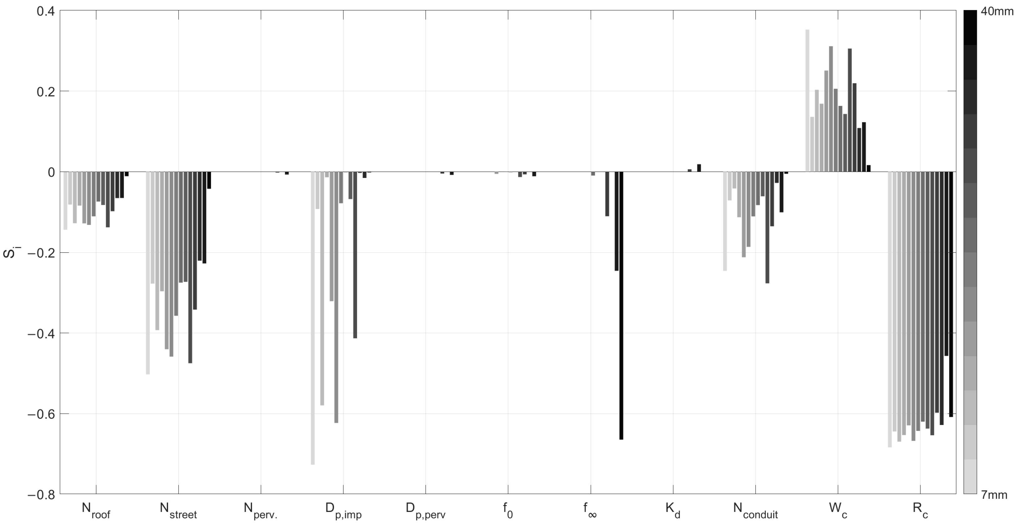
2.2.2. Sensitivity Analysis

A local sensitivity analysis was conducted by changing once-at-a-time each parameter from a reference value to a minimum and maximum in a predefined range of variation, and the impact on the global variables, peak discharge (Q_p), and total volume (V_t) for all the considered rainfall events, was investigated. The reference value of the parameters and their respective range of variation are listed in

Table 3. List of parameters considered for the sensitivity analysis and corresponding range of variations.

Parameter	Symbol	Reference Value	Range of Variation
Manning coefficient roofs	$N_{roof}$	0.020	[0.014–0.30]
Manning coefficient streets	$N_{street}$	0.014	[0.010–0.055]
Manning coefficient pervious area	$N_{perv}$	0.15	[0.10–0.35]
Depression storage impervious area	$D_{p,imp}$	1.35	[0.00–2.54]
Depression storage pervious area	$D_{p,perv}$	2.60	[2.54–5.08]
Maximum infiltration rate	$f_0$	117.00	[58.00–170.00]
Minimum infiltration rate	$f_{\infty }$	17.00	[1.00–57.00]
Decay coefficient	$K_d$	5.34	[2.00–7.00]
Manning coefficient conduit	$N_{conduit}$	0.0147	[0.0120–0.0200]
Width coefficient	$W_c$	1.50	[1.00–2.00]
Percent routed	$R_c$	25.00	[0.00–50.00]

and taken from [5,28]. To quantify the sensitivity of the model outputs to parameter variations, the following sensitivity index (S_i), to be evaluated for the i-th parameter and for all the rainfall events, was introduced:

$$S_i={\displaystyle \frac{U_{up}-U_{low}}{U^{*}}}$$

(3)

where $U_{up}$ and $U_{low}$ are the global variable values obtained by setting the i-th parameter to the upper and lower value of the range of variation, respectively. $U^{*}$ is the global variable value when the reference value for all the parameters is set. Values close to zero for the sensitivity index indicate a negligible impact of the i-th parameter. Positive values of S_i show a consistent impact of the parameter (increasing/decreasing the parameter leads to increasing/decreasing the output). Conversely, negative values show an inverse effect of the parameter. Parameters showing low values of this index can be set to a constant value (e.g., equal to a reference value) and not included in the calibration process.

2.2.3. Genetic Optimization

A Genetic Algorithm (GA) framework was used in this work for the event-based calibration of the hydrologic/hydraulic model of the Cascina Scala catchment. Notably, decision variables are the previously defined parameters (see Table 3) for the 42 sub-catchments to be optimized for each of the fourteen selected rainfall events. These decision variables represent the genes of the individuals (possible solutions to the optimization problem) and constitute a single population [15]. GA defines the initial population randomly. Then, through crossover and mutation processes, it evolves towards an optimum solution expressed through an objective function (OF). In this work, the goal was to maximize the fit of modeled-to-measured hydrographs at the basin closing section singularly for each of the selected rainfall events. Accordingly, the OF (to be minimized) was expressed as in the following:

$$OF={\displaystyle \frac{1}{n}}{\displaystyle \sum }_{i=1}^n{\left(Q_{s,i}-Q_{m,i}\right)}^2$$

(4)

where n is the number of time instants in the generic rainfall event (in this study, temporal resolution for rainfall/discharge is 1 min), while $Q_{s,i}\left({\displaystyle \frac{L}{s}}\right)$ and $Q_{m,i} \left({\displaystyle \frac{L}{s}}\right)$ stand for simulated and measured water discharge at the generic i-th time instant, respectively, in the generic rainfall event.

Furthermore, in order to assess the possible benefit of carrying out a preliminary sensitivity analysis in terms of computational cost and calibration performance, in this work, two kinds of optimization were performed:

-

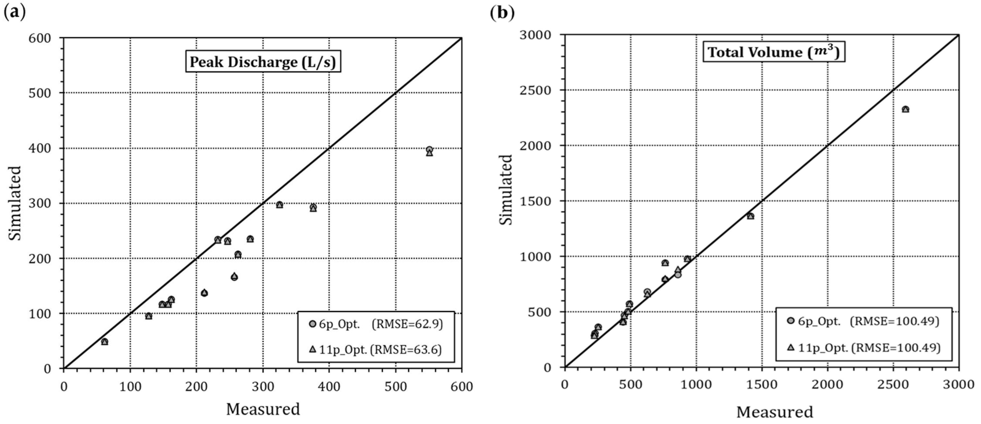
Calibration 1: all the defined parameters are considered in the optimization (in this work, 11 parameters);

-

Calibration 2: only the most impactful parameters on the model outputs (as from the sensitivity analysis) are considered in the optimization, while considering the other parameter value constant and equal to the reference value (Table 3).

The GA toolbox of MATLAB^® R2023b was linked to the EPA-SWMM dll for the calibration process.

2.2.4. Goodness-of-Fit

Three goodness-of-fit indices were used for assessing the calibration performance: (1) the Root Mean Square Error (RMSE), the lower, the better; (2) the coefficient of determination (R²), the higher, the better; and (3) the percentage relative error (E_r), the closer to zero, the better.

$$RMSE=\sqrt{{\displaystyle \frac{1}{n}}{\displaystyle \sum }_{i=1}^n{\left(Y_{m,i}-Y_{s,i}\right)}^2}$$

(5)

$$R^2={\displaystyle \frac{{\sum }_{i=1}^n{\left(Y_{s,i}-\overline{Y_m}\right)}^2}{{\sum }_{i=1}^n{\left(Y_{m,i}-\overline{Y_m}\right)}^2}}$$

(6)

$$E_r={\displaystyle \frac{Y_s-Y_m}{Y_m}}\ast 100$$

(7)

where $\overline{Y_m}$ is the mean value of the measured variable $Y_{m,i}$, $Y_{s,i}$ is the simulated values, and n is the number of time instants (if the index is calculated on the single full hydrograph), or it is equal to the total number of considered rainfall events (if the index is calculated referring to the global variables measured $\left(Y_m\right)$ and simulated $\left(Y_s\right)$ peak discharge and total volume).

3. Results

Results of all simulation’s SA, by varying the values of the parameters in the corresponding sampling range (Table 3) for the fourteen rainfall events, are represented in Figure 3 (regarding the impact on peak discharge) and Figure 4 (regarding the impact on total volume). Each group of histogram bars of sensitivity indices relates to a single parameter, while each bar stands for the specific value of the sensitivity index corresponding to a specific rainfall event. Bar heights show the influence of each parameter involved in SA. Indices are ordered based on ascending event-depth values.

Even if local SA does not allow evaluation of the effects of nonlinear interactions between different parameters, which unavoidably rule most of the modeled hydrological processes (e.g., Equation (2)), results are still clear. Nonlinearity of the processes considered can be detected, for example, from the nonlinear (and sometimes not-monotonic) trends of the variation in the sensitivity indices for some parameters as the rainfall depth increases. Furthermore, as they were analyzed, results from the performed SA also suggest the type of impact (positive/negative), making them more explicative.

It is clear that peak flow and total runoff volume have different sensitivities to parameters changing as the total rainfall depth of the event changes. This points out the importance of rainfall characteristics in assessing the impact of a parameter on model output.

SA shows that considering both peak flow and total volume, among the eleven considered parameters, only six of them have a significant impact on the simulation outputs in all the fourteen rainfall events (namely, $N_{roof}$, $N_{street}$, $D_{p,imp}$, $N_{conduit}$, $W_c$, and $R_c$), and with minimum infiltration rate ($f_{\infty }$) becoming more influential just for a few events (increasingly for those featuring the highest value of rainfall depth). This shows that as the event total rainfall depth increases, the weight of the infiltration process in the pervious area becomes more influential.

Furthermore, as the total rainfall depth increases, the influence of the six most important parameters decreases (more marked on total volume), except for R_c, which shows the highest, constant importance.

The most important parameters were those referring to impervious areas and the coefficient W_c for the equivalent width of the contributing runoff area. This means that, whatever the values of D_p,perv and N_perv within the investigated ranges, the considered rainfall events feature such a low rainfall depth that no runoff is generated from pervious areas, maybe due to infiltration. W_c shows a positive impact on both outputs (increasing W_c results in a more enlarged shape of sub-catchments, faster overland flow, and then a reduction in infiltration); the other five important parameters show a negative impact. For example, an increase of D_p,imp and R_c, contributes to reducing the excess rainfall (interception and infiltration due to routing on pervious area phenomena, respectively) and then peak discharge and volume. For larger total rainfall depths, impervious area parameters’ importance decreases due to the occurrence of surface saturation, and for example, $D_{p,imp}$ becomes less impactful because of the rapid filling of storage capacities.

According to the SA results, only the six most important parameters (for all the analyzed rainfall events) were kept for the second kind of optimization, namely calibration 2.

Subsequently, the comparison between calibration 1 (eleven-parameter optimization, 11p_Opt.) and calibration 2 (six-parameter optimization, 6p_Opt.) was performed to understand the influence of pre-selection of meaningful parameters. Calibrated values are listed in

Table 4. Calibrated parameters for both kinds of optimization for all fourteen rainfall events. In bold, the most important parameters as selected through sensitivity analysis.

Parameters	Opt.	Events
		3	5	7	8	9	11	12	13	14	17	19	20	21	23
${\mathit{N}}_{\mathit{r}\mathit{o}\mathit{o}\mathit{f}}$	6p	0.014	0.014	0.014	0.014	0.014	0.014	0.014	0.014	0.014	0.014	0.014	0.016	0.014	0.014
	11p	0.014	0.014	0.014	0.014	0.014	0.014	0.014	0.014	0.014	0.014	0.014	0.014	0.014	0.014
${\mathit{N}}_{\mathit{s}\mathit{t}\mathit{r}\mathit{e}\mathit{e}\mathit{t}}$	6p	0.010	0.010	0.010	0.010	0.010	0.010	0.010	0.010	0.010	0.010	0.010	0.010	0.010	0.010
	11p	0.010	0.010	0.010	0.010	0.010	0.010	0.010	0.010	0.010	0.010	0.010	0.010	0.010	0.010
$N_{perv}$	11p	0.21	0.31	0.31	0.34	0.32	0.13	0.15	0.18	0.10	0.34	0.22	0.10	0.26	0.15
${\mathit{D}}_{\mathit{p},\mathit{i}\mathit{m}\mathit{p}}$	6p	0.00	0.95	0.00	1.85	2.54	0.85	0.47	0.56	0.17	2.54	2.37	0.02	0.13	0.90
	11p	0.00	0.66	0.00	1.95	2.54	0.88	0.46	0.54	0.21	2.54	2.37	0.00	0.16	0.91
$D_{p,perv}$	11p	4.20	4.58	4.43	3.96	4.22	5.04	4.06	3.61	2.54	4.44	3.89	2.54	4.36	3.87
$f_0$	11p	101.93	161.68	116.14	78.22	71.11	70.14	152.32	153.11	58.00	73.91	164.30	58.00	85.57	59.25
$f_{\infty }$	11p	47.46	21.26	51.38	50.53	51.45	22.13	46.85	40.66	1.01	25.96	54.85	6.84	50.17	20.73
$K_d$	11p	6.17	3.10	5.27	5.06	3.99	2.75	3.09	2.83	7.00	6.17	5.30	7.00	2.57	5.62
${\mathit{N}}_{\mathit{c}\mathit{o}\mathit{n}\mathit{d}\mathit{u}\mathit{i}\mathit{t}}$	6p	0.0120	0.0137	0.0120	0.0139	0.0120	0.0138	0.0120	0.0120	0.0121	0.0127	0.0120	0.0197	0.0120	0.0120
	11p	0.0121	0.0146	0.0120	0.0138	0.0120	0.0138	0.0120	0.0120	0.0120	0.0129	0.0121	0.0186	0.0121	0.0120
${\mathit{W}}_{\mathit{c}}$	6p	2.00	2.00	2.00	2.00	2.00	2.00	2.00	2.00	2.00	2.00	2.00	2.00	2.00	2.00
	11p	2.00	2.00	2.00	2.00	2.00	2.00	2.00	2.00	2.00	2.00	2.00	2.00	2.00	2.00
${\mathit{R}}_{\mathit{c}}$	6p	8.99	0.00	6.00	0.00	13.59	0.00	0.00	0.00	0.00	24.66	14.71	27.31	43.83	0.00
	11p	9.39	0.00	6.12	0.00	13.26	0.00	0.00	0.00	0.01	24.59	14.73	36.24	43.21	0.00

. Notably, for the less impactful parameters (N_perv, D_p,perv, $f_0, f_{\infty }$, and K_d) results are listed only for the 11p_Opt.

The results show that for the 6p_Opt., even by neglecting the non-influential parameters in the calibration step and considering them as constant values (equal to their reference values, as shown in Table 3), the calibrated values of influential parameters are equal (N_roof, N_street, W_c) or just slightly different (D_p,perv, N_conduit, R_c) from those obtained for the 11p_Opt. in most of the cases.

As an example, the hydrographs (and the corresponding hyetographs in black histograms) for events 3, 12, 17, and 23 (with different features and duration ranging from 196 min to 1131 min) are plotted in Figure 5 for the 11p_Opt. (light gray solid line) and the 6p_Opt. (dark gray solid line) optimizations. Measured data are highlighted with rectangular black symbols. Results from both calibrations were in good agreement with the measured data, with a slight underestimation of the peak flow and an even less overestimation of the total runoff volume. It is evident from the hydrographs and from the RMSE values that the two calibration methods lead to very similar results.

In

Table 5. Simulation results in terms of goodness-of-fit for the 14 rainfall events.

Event	R2		RMSE		Er,peak		Er,vol
	6p	11p	6p	11p	6p	11p	6p	11p
3	0.89	0.89	18.00	18.09	−5.93	−6.52	17.30	16.82
5	0.89	0.89	35.56	35.55	−27.87	−28.80	3.58	5.10
7	0.63	0.63	56.44	56.53	−8.48	−8.73	33.20	33.02
8	0.86	0.86	35.39	35.37	−21.95	−22.48	3.26	2.37
9	0.80	0.80	16.23	16.24	−22.29	−22.01	44.18	44.73
11	0.94	0.94	14.35	14.36	−15.97	−16.03	−3.53	−3.68
12	0.90	0.90	15.94	15.95	−20.84	−20.88	4.47	4.58
13	0.83	0.83	20.47	20.49	−25.51	−25.54	−8.05	−7.72
14	0.88	0.90	16.50	15.18	−35.32	−34.37	−3.01	2.93
17	0.87	0.87	8.03	8.04	−25.61	−25.60	23.15	23.24
19	0.97	0.97	9.59	9.63	1.05	0.77	5.40	5.31
20	0.78	0.81	22.11	20.78	−35.38	−34.64	8.50	5.81
21	0.85	0.85	5.16	5.16	−20.71	−19.85	27.56	28.49
23	0.93	0.93	11.34	11.34	−20.86	−20.86	−10.20	−10.22

, the values of the three goodness-of-fit indices (Section 2.2.4) are listed for all the events and for both types of calibrations, calculated considering the measured and simulated hydrograph at the catchment outlet, peak flow, and total volume. It is evident that the value of R² is generally high for all the events and very similar for the two kinds of calibration, and RMSE values are generally small, with the highest values for events 5, 7, and 8, namely for the most extreme events (events characterized by the highest average rainfall intensity, as shown in Table 2). In terms of global performance, it is confirmed that for all the events, the two calibrations perform similarly, with a general underestimation of the peak flow and overestimation of the total volume (as can be seen from the negative/positive values of E_r,peak/E_r,vol, respectively, in Table 5).

Table 6. Computational cost for both kinds of calibrations. In bold, events for which the 6p_Opt. requires lower time than 11p_Opt.

Event	Opt.	n° Gen.	n° F_eval.	Event	Opt.	n° Gen.	n° F_eval.
3	6p	247	47,140	13	6p	168	32,130
	11p	155	29,660		11p	159	30,420
5	6p	205	39,160	14	6p	266	50,750
	11p	279	53,220		11p	312	59,490
7	6p	230	43,910	17	6p	155	29,660
	11p	169	32,320		11p	179	34,220
8	6p	223	42,580	19	6p	212	40,490
	11p	248	47,330		11p	203	38,780
9	6p	203	38,780	20	6p	171	32,700
	11p	231	44,100		11p	502	95,590
11	6p	161	30,800	21	6p	168	32,130
	11p	214	40,870		11p	365	69,560
12	6p	228	43,530	23	6p	205	39,160
	11p	190	36,310		11p	227	43,340

shows the computational cost of both types of calibration for each rainfall event. It is expressed in terms of number of generations (n° Gen.) and cumulative number of function evaluations (n° F_eval.) required by the optimization algorithm for calibrating the model (i.e., defining the optimal parameters’ values) through the minimization of the objective function (Equation (5)) till the stopping criterion is reached (the average change in the fitness value is less than the set function tolerance of 10⁻⁶). The results show that in most events (nine out of fourteen rainfall events), the 6p_Opt. requires a lower number of generations (n° Gen.) and a lower number of function evaluations (n° F_eval.) than 11p_Opt. In two of the remaining cases (namely, events 13 and 19), the difference is around 10 generations. Furthermore, for the events 20 and 21, the 6p_Opt. is almost three and two times faster than 11p_Opt., respectively. Thus, utilizing a reduced set of parameters for the calibration step demonstrates a significant decrease in computational costs and, consequently, in the computational time while maintaining reliable model performance. This is particularly advantageous for applications requiring rapid decision-making. Optimizations were run by using MATLAB R2023b linked to SWMM 5.1 on a Windows 11Pro-23H2 PC with a 3.20 GHz Intel(R) Core(TM) i9-14900KF CPU and 4.00 GB of RAM.

In Figure 6, a comparison between the performance of the 11p_Opt. (grey triangle symbols) and 6p_Opt. (grey circle symbols) is shown in terms of peak discharge (Figure 6a) and total volume (Figure 6b). The RMSE was also calculated for the total volume and the peak discharge, considering both calibrations and the fourteen rainfall events. The dots aligned along the bisector for both calibrations confirm a similar behavior and good performance both in terms of peak flow (RMSE = 62.9 L/s and RMSE = 63.6 L/s for 6p_Opt. and 11p_Opt., respectively) and total volume (RMSE = 100.5 m³ for both calibrations). It is even more evident from Figure 6 that both calibrations underestimated the peak discharge (especially for events characterized by higher values) while just slightly overestimating the total volume in all but one case. This may call for future investigations about the need for higher modeling spatial resolution or for different objective functions in the calibration step that could favor the fitting of the model to the highest experimental observation values.

4. Discussion

The findings of this study are a key contribution to the understanding of sensitivity analysis for improving calibration performance in urban hydrological modeling by using EPA-SWMM 5.1 software. Results are in agreement with the literature, underlining the crucial role of sensitivity analysis in identifying the most influential parameters in hydrological modeling [9,29,30]. Linking sensitivity analysis with genetic algorithm optimization has shown that a smaller set of parameters, properly identified, allows effective calibration of urban drainage models without loss in the accuracy of the results and by saving computational cost. Results satisfactorily agreed with the measured data for all the considered rainfall events, confirming the good performance of the EPA-SWMM 5.1 software. Interestingly, it emerges from the results that good calibration of the model can be obtained without having detailed knowledge of the soil characteristics (for the infiltration Horton model parameters), which results in an important benefit in terms of cost/time saving for the related field investigations. On the other hand, the crucial role played by the impervious area parameters (Manning coefficient and depression storage), especially for short-duration events, is confirmed and in line with the literature [22,31,32,33]. Similarly, the slightly increasing sensitivity to infiltration rates occurring during events with longer durations and higher rainfall depths shows consistency with the findings of [22]. In general, results show a high dependence of model output sensitivity on the rainfall features (i.e., total rainfall depth). This further points out the crucial importance of a proper calibration of urban drainage models and the fact that catchment behavior is actually the resulting effect of the combined response of rainfall/area characteristics. This is also confirmed by the different values assumed by some calibrated parameters for different rainfall events, like D_p,imp, and R_c (see Table 4), both regarding impervious area features and strongly impacting the catchment response in terms of hydrological losses. This translates, on the other hand, into the critical impact of catchment urbanization/imperviousness and into the reliable definition of related parameters (namely, percentage, type, and routing processes).

It is worth noting that focusing on the most sensitive parameters can result in more reliable model performance, as also emphasized in [22,34]. In this regard, the 6p_Opt. outperformed the 11p_Opt. with a value of RMSE for peak discharge of 62.9 L/s against 63.6 L/s and an almost identical RMSE value for the total runoff volume. This clearly shows that an increase in the number of parameters does not necessarily entail better model performance. On the contrary, it can result in over-parameterization at the expense of computational efficiency. It can also be observed that, for both calibration approaches, the highest values of RMSE (see Table 5) were obtained for the three shortest duration events (5, 7, and 8), which may be due to the assumption of uniform rainfall spatial distribution over the catchment, which may not hold true for short/intense rainfall events.

The implications of such findings are impactful. The efficiency of reduced-parameter calibration demonstrated here has direct applications in real-time urban stormwater management, where computational efficiency is crucial. Moreover, the results of this study show how parameter importance varies depending on rainfall characteristics, which provides a good basis for adaptive calibration strategies for different rainfall events. This is particularly the case when considering climate change, where future rainfall is predicted to alter its patterns and increase intensities that could potentially lead to increased urban flood risk.

Future research directions could be dedicated to the adoption of global sensitivity analysis techniques, although computationally expensive, which may give deeper insights into the parameters intercorrelation and (nonlinear) interactions between them and their combined effects on hydrological outputs for a better selection of the most impactful parameters, especially for more complicated modeling with numerous parameters to be optimized. In addition, future studies could concern catchments from different geographical and climatic areas for assessing the generalizability of the findings in terms of parameter selection and of computation and reliability benefits for the subsequent calibration step. In this regard, the present study contributes to the developing literature on urban hydrological modeling by providing a practical and efficient methodology for sensitivity analysis-aided calibration. Results corroborate the trade-off between modeling complexity and model accuracy/explicability, proving that models with fewer, properly selected optimized parameters can outperform more complex ones.

References

1. Zhu, Z.; Morales, V.; Garcia, M.H. Impact of Combined Sewer Overflow on Urban River Hydrodynamic Modelling: A Case Study of the Chicago Waterway. Urban Water J. 2017, 14, 984–989. [Google Scholar] [CrossRef]
2. Kourtis, I.M.; Tsihrintzis, V.A. Adaptation of Urban Drainage Networks to Climate Change: A Review. Sci. Total Environ. 2021, 771, 145431. [Google Scholar] [CrossRef]
3. Todeschini, S. Trends in Long Daily Rainfall Series of Lombardia (Northern Italy) Affecting Urban Stormwater Control. Int. J. Climatol. 2012, 32, 900–919. [Google Scholar] [CrossRef]
4. Skotnicki, M.; Sowiński, M. The Influence of Depression Storage on Runoff from Impervious Surface of Urban Catchment. Urban Water J. 2015, 12, 207–218. [Google Scholar] [CrossRef]
5. Giudicianni, C.; Assaf, M.N.; Todeschini, S.; Creaco, E. Comparison of Nonlinear Reservoir and UH Algorithms for the Hydrological Modeling of a Real Urban Catchment with EPASWMM. Hydrology 2023, 10, 24. [Google Scholar] [CrossRef]
6. Arseni, M.; Rosu, A.; Calmuc, M.; Calmuc, V.A.; Iticescu, C.; Georgescu, L.P. Development of Flood Risk and Hazard Maps for the Lower Course of the Siret River, Romania. Sustainability 2020, 12, 6588. [Google Scholar] [CrossRef]
7. Assaf, M.N.; Manenti, S.; Creaco, E.; Giudicianni, C.; Tamellini, L.; Todeschini, S. New Optimization Strategies for SWMM Modeling of Stormwater Quality Applications in Urban Area. J. Environ. Manag. 2024, 361, 121244. [Google Scholar] [CrossRef] [PubMed]
8. Niazi, M.; Nietch, C.; Maghrebi, M.; Jackson, N.; Bennett, B.R.; Tryby, M.; Massoudieh, A. Storm Water Management Model: Performance Review and Gap Analysis. J. Sustain. Water Built Environ. 2017, 3, 04017002. [Google Scholar] [CrossRef]
9. Hashemi, M.; Mahjouri, N. Global Sensitivity Analysis-Based Design of Low Impact Development Practices for Urban Runoff Management Under Uncertainty. Water Resour. Manag. 2022, 36, 2953–2972. [Google Scholar] [CrossRef]
10. Wang, W.-C.; Cheng, C.-T.; Chau, K.-W.; Xu, D.-M. Calibration of Xinanjiang Model Parameters Using Hybrid Genetic Algorithm Based Fuzzy Optimal Model. J. Hydroinformatics 2012, 14, 784–799. [Google Scholar] [CrossRef]
11. Liu, Y.; Batelaan, O.; De Smedt, F.; Poórová, J.; Velcick, L. Automated Calibration Applied to a GIS-Based Flood Simulation Model Using PEST. In Floods, from Defence to Management: Symposium Proceedings of the 3rd International Symposium on Flood Defence, Nijmegen, The Netherlands, 25–27 May 2005; van Alphen, J., van Beek, E., Taal, M., Eds.; Taylor & Francis Group: London, UK, 2005. [Google Scholar]
12. Alamdari, N. Development of a Robust Automated Tool for Calibrating a SWMM Watershed Model. In Proceedings of the World Environmental and Water Resources Congress 2016, American Society of Civil Engineers, West Palm Beach, FL, USA, 22–26 May 2016; pp. 221–228. [Google Scholar]
13. Barco, J.; Wong, K.M.; Stenstrom, M.K. Automatic Calibration of the U.S. EPA SWMM Model for a Large Urban Catchment. J. Hydraul. Eng. 2008, 134, 466–474. [Google Scholar] [CrossRef]
14. Shahed Behrouz, M.; Zhu, Z.; Matott, L.S.; Rabideau, A.J. A New Tool for Automatic Calibration of the Storm Water Management Model (SWMM). J. Hydrol. 2020, 581, 124436. [Google Scholar] [CrossRef]
15. Holland, J.H. Genetic Algorithms and the Optimal Allocation of Trials. SIAM J. Comput. 1973, 2, 88–105. [Google Scholar] [CrossRef]
16. Chlumecký, M.; Buchtele, J.; Richta, K. Application of Random Number Generators in Genetic Algorithms to Improve Rainfall-Runoff Modelling. J. Hydrol. 2017, 553, 350–355. [Google Scholar] [CrossRef]
17. Duarte Lopes, M.; Barbosa Lima da Silva, G. An Efficient Simulation-Optimization Approach Based on Genetic Algorithms and Hydrologic Modeling to Assist in Identifying Optimal Low Impact Development Designs. Landsc. Urban Plan. 2021, 216, 104251. [Google Scholar] [CrossRef]
18. Song, X.; Zhan, C.; Kong, F.; Xia, J. Advances in the Study of Uncertainty Quantification of Large-Scale Hydrological Modeling System. J. Geogr. Sci. 2011, 21, 801–819. [Google Scholar] [CrossRef]
19. Lenhart, T.; Eckhardt, K.; Fohrer, N.; Frede, H.-G. Comparison of Two Different Approaches of Sensitivity Analysis. Phys. Chem. Earth Parts A/B/C 2002, 27, 645–654. [Google Scholar] [CrossRef]
20. Bahremand, A.; De Smedt, F. Distributed Hydrological Modeling and Sensitivity Analysis in Torysa Watershed, Slovakia. Water Resour. Manag. 2008, 22, 393–408. [Google Scholar] [CrossRef]
21. Saltelli, A.; Chan, K.; Scott, M. Sensitivity Analysis; John Wiley & Sons, Ltd.: New York, NY, USA, 2000. [Google Scholar]
22. Giudicianni, C.; Di Cicco, I.; Di Nardo, A.; Greco, R. Variance-Based Global Sensitivity Analysis of Surface Runoff Parameters for Hydrological Modeling of a Real Peri-Urban Ungauged Basin. Water Resour. Manag. 2024, 38, 3007–3022. [Google Scholar] [CrossRef]
23. Song, X.; Zhang, J.; Zhan, C.; Xuan, Y.; Ye, M.; Xu, C. Global Sensitivity Analysis in Hydrological Modeling: Review of Concepts, Methods, Theoretical Framework, and Applications. J. Hydrol. 2015, 523, 739–757. [Google Scholar] [CrossRef]
24. Hamby, D.M. A Review of Techniques for Parameter Sensitivity Analysis of Environmental Models. Environ. Monit. Assess. 1994, 32, 135–154. [Google Scholar] [CrossRef] [PubMed]
25. Barco, J.; Papiri, S.; Stenstrom, M.K. First Flush in a Combined Sewer System. Chemosphere 2008, 71, 827–833. [Google Scholar] [CrossRef] [PubMed]
26. Creaco, E.; Todeschini, S.; Franchini, M. Hydrological Modelling of the Cascina Scala Catchment. EPiC Ser. Eng. 2018, 3, 495–503. [Google Scholar]
27. Rossman, L.; Huber, W. Storm Water Management Model Reference Manual Volume I-Hydrology (Revised); US Environmental Protection Agency: Cincinnati, OH, USA, 2016. [Google Scholar]
28. Rossman, L. Storm Water Management Model User’s Manual Version 5.0; US Environmental Protection Agency: Cincinnati, OH, USA, 2010. [Google Scholar]
29. Del Giudice, G.; Padulano, R. Sensitivity Analysis and Calibration of a Rainfall-Runoff Model with the Combined Use of EPA-SWMM and Genetic Algorithm. Acta Geophys. 2016, 64, 1755–1778. [Google Scholar] [CrossRef]
30. Fatone, F.; Szelag, B.; Kiczko, A.; Majerek, D.; Majewska, M.; Drewnowski, J.; Łagód, G. Advanced Sensitivity Analysis of the Impact of the Temporal Distribution and Intensity of Rainfall on Hydrograph Parameters in Urban Catchments. Hydrol. Earth Syst. Sci. 2021, 25, 5493–5516. [Google Scholar] [CrossRef]
31. Ballinas-González, H.A.; Alcocer-Yamanaka, V.H.; Canto-Rios, J.J.; Simuta-Champo, R. Sensitivity Analysis of the Rainfall–Runoff Modeling Parameters in Data-Scarce Urban Catchment. Hydrology 2020, 7, 73. [Google Scholar] [CrossRef]
32. Rabori, A.M.; Ghazavi, R.; Reveshty, M.A. Sensitivity Analysis of SWMM Model Parameters for Urban Runoff Estimation in Semi-Arid Area. J. Biodivers. Environ. Sci. 2017, 10, 284–294. [Google Scholar]
33. Gong, Y.; Li, X.; Zhai, D.; Yin, D.; Song, R.; Li, J.; Fang, X.; Yuan, D. Influence of Rainfall, Model Parameters and Routing Methods on Stormwater Modelling. Water Resour. Manag. 2018, 32, 735–750. [Google Scholar] [CrossRef]
34. Xu, Z.; Xiong, L.; Li, H.; Xu, J.; Cai, X.; Chen, K.; Wu, J. Runoff Simulation of Two Typical Urban Green Land Types with the Stormwater Management Model (SWMM): Sensitivity Analysis and Calibration of Runoff Parameters. Environ. Monit. Assess. 2019, 191, 343. [Google Scholar] [CrossRef] [PubMed]
Figure 1. General view of Cascina Scala catchment.
Water 17 00612 g001
Figure 2. Flow chart of research methodology.
Water 17 00612 g002
Figure 3. Sensitivity indices for peak discharge for the 14 events sorted based on the total rainfall depth.
Water 17 00612 g003
Figure 4. Sensitivity indices for total volume for the 14 events sorted based on the total rainfall depth.
Water 17 00612 g004
Figure 5. Hyetographs (black histograms) and comparison of the hydrographs for 11p_Opt. (light gray solid line) and 6p_Opt. (dark gray solid line) calibrations with measured data (black rectangular symbol) for (a) event 3; (b) event 12; (c) event 17; and (d) event 23.
Water 17 00612 g005
Figure 6. Comparison plot between measured and simulated global variables for the 11p_Opt. (grey triangle symbols) and the 6p_Opt. optimization (grey circle symbols) in terms of (a) peak discharge and (b) total volume.
Water 17 00612 g006