Abstract
Due to the uncertainty of meteorological factors and the influence of human activities, the monthly runoff series often exhibit the characteristics of non-stationarity. The appropriate prediction model and the hyperparameters of the model are often difficult to determine, and this affects the model prediction performance. For obtaining the accurate runoff prediction results, a novel prediction model (KVMD-KTCN-LSTM-SA) is proposed. This hybrid model uses Kepler optimization algorithm (KOA)-optimized Variable Mode Decomposition (KVMD), KOA-optimized temporal convolutional network–long short-term memory (TCN-LSTM), and the self-attention (SA) mechanism. KVMD effectively reduces the difficulty of predicting the monthly runoff series, KOA helps to find the optimal hyperparameters of the model, TCN is combined with LSTM, and the SA mechanism effectively increases the performance of the model. Monthly runoff from three hydrological stations in the Hetian River basin and one hydrological station in the Huaihe River basin are predicted with the proposed model, and six models are selected for comparison. The KVMD-KTCN-LSTM-SA model effectively reduces runoff fluctuation and combines the advantages of multiple models and achieves satisfactory runoff prediction results. During the testing period, the proposed model achieves NSE of 0.978 and R2 of 0.982 at Wuluwati station, NSE of 0.975 and R2 of 0.986 at Tongguziluoke station, and NSE of 0.978 and R2 of 0.982 at Jiangjiaji station. The proposed hybrid model provides a new approach for monthly runoff prediction, which is capable of better managing and predicting mid-long-term runoff.
1. Introduction
With the change in global meteorology and the impact of human activities such as the construction of hydropower stations on rivers and urbanization, floods and droughts are becoming more and more frequent, and the runoff series exhibits non-stationary characteristics [1,2]. Surface runoff, as an important part of the water cycle, has been the focus of research [3]. Accurate and reliable monthly runoff prediction is significant for stable socio-economic development, safe operation of reservoirs, and water resource allocation in the basin [4,5].
Typically, runoff prediction models are divided into process-driven models and data-driven models. Process-driven models describe the relationship between rainfall and runoff accurately [6], and the modeling process has real physical meaning [7]. However, this method is time-consuming for parameter tuning, and it is difficult to obtain satisfactory runoff simulation results in the face of data shortages [8]. Data-driven models are easy to use, and this kind of approach has achieved great results in many fields. In areas where actual data are not sufficient, such models can produce satisfactory runoff predictions [9]. The utilization of neural network models in the domain of runoff simulation has become a new trend in runoff prediction with the continuous advancement of computer technology. Among the neural network models, LSTM has been successfully applied to the Huaihe River basin, which captures the nonlinear characteristics of runoff changes well [10]. Gated Recurrent Unit (GRU), as a variant model of LSTM with less training time and a simple model structure, has been successfully applied in short-term runoff prediction [11]. TCN allows parallel feature processing and is an effective prediction tool [12]. Support vector machine (SVM), as an effective prediction model with good generalization ability, has achieved good results in predicting weak non-stationary runoff series [13]. These single models have demonstrated some capability in runoff series prediction. However, they are not well-suited to dealing with highly nonlinear series and are unable to adequately identify and extract the changing features of the series. Currently, hybrid models are receiving increasing attention from scholars, which can overcome the limitations of single models and better capture the characteristics of runoff changes. One class of hybrid models is the combination of optimization algorithms to find the optimal hyperparameters of the models, this facilitates better time series modeling and reduces the time spent on tuning the parameters. Sparrow Search Algorithm (SSA) [14], Harris Hawk Optimization (HHO) [15], Particle Swarm Optimization (PSO) [16], etc., have been applied to runoff prediction and have achieved better prediction results than unoptimized models. The Kepler optimization algorithm, as a robust physics-based metaheuristic algorithm with strong optimality finding capability, has been applied with results in several fields [17].
Another type of runoff hybrid prediction model is improved by combining the data preprocessing methods to enhance the accuracy, and the core of this type of model is the idea of “decomposition-integration”. Common decomposition methods in runoff prediction include empirical mode decomposition (EMD), ensemble empirical mode decomposition (EEMD), etc. [18,19]. After the runoff data are decomposed by EMD, the modified EMD-SVM model is improved by deleting IMF 1, which obtains accurate prediction in the Weihe River basin [20]. The EEMD combined with the ANN model could simulate the runoff process during flood season well [21]. VMD is an efficient signal processing method that decomposes a signal into non-recursive variational problems. It is robust to signal noise and able to decompose the signal into intrinsic mode functions (IMFs) with different center frequencies; to a certain extent, the problem of modal aliasing in EMD and EEMD has been solved [22]. VMD combined with BiLSTM successfully predicted the DEDI index for meteorological drought, and VMD combined with a two-stage decomposition strategy improved the prediction accuracy of annual runoff in the Lechang Valley watershed [23,24].
Combining optimization algorithms and preprocessing methods can lead to more accurate runoff prediction results [25]. Also, the addition of a self-attention mechanism to the neural network structure is a useful approach. This can help the model to capture global dependencies and improve parallelization [26].
KOA has better performance than pelican optimization algorithm (POA), slime mold algorithm (SMA), and other algorithms, and it can solve some practical engineering problems well [27]. The VMD algorithm is often used for data preprocessing, but the number of decomposition layers and iterations are difficult to determine [28]. In addition, TCN-LSTM has been shown to have better performance than the commonly used models for runoff prediction such as LSTM and TCN [29]. In consideration of the precision of machine learning models for mid-long-term runoff series prediction, a novel KVMD-KTCN-LSTM-SA monthly runoff prediction model is proposed, which combines the KOA, TCN-LSTM, VMD, and SA mechanism. Firstly, the model uses the KOA to optimize the VMD parameters and then employs the KVMD to decompose the runoff series. This approach addresses the challenge of selecting appropriate VMD parameters. Second, the SA mechanism is added to the TCN-LSTM model, and the KOA is used to find the optimal hyperparameters of this model. Thirdly, different IMFs are predicted with the KTCN-LSTM-SA model, and the final monthly runoff prediction is obtained by summing up the predictions of the IMFs.
The main contributions of this study are as follows:
- (1)
- A novel KVMD-KTCN-LSTM-SA prediction model is proposed. The KVMD reduces the complexity of the original runoff, and the SA mechanism allows the model to better capture global dependencies and improve parallelization.
- (2)
- The KOA combined with the TCN-LSTM model quickly finds the optimal hyperparameters. This makes full use of TCN’s ability to extract multi-scale features and the capacity of LSTM to capture long-term dependencies.
- (3)
- The proposed KVMD-KTCN-LSTM-SA model is applied to three hydrological stations in the Hotan River basin and Huai River basin with six comparative models. The applicability of this model and the excellent monthly runoff prediction capability are demonstrated by four evaluation indicators.
2. Materials and Methods
2.1. Datasets
The Hotan River basin is in northwestern China, in the southwestern part of the Tarim Basin (77°25′–81°43′ E, 34°52′–40°28′ N), with a total basin area of 4.9 × 10⁴ km2. The basin has a temperate continental climate, with an average annual precipitation of 39.6 mm and an average annual evaporation of 2882.6 mm [30]. The landscape of the basin is high in the south and low in the north, with the lowest elevation in the basin being 1275 m and the highest elevation being 6855 m, and the southern part of the basin is a high mountainous area, with an average elevation of more than 3000 m. The northern part of the basin is a hilly area with gentle terrain and an open riverbed. The Hotan River consists of two tributaries, the Yulongkashi River and the Kalakashi River, which flow through the Tongguziluoke station and the Wuluwati station, respectively, and merge downstream. The Yulongkashi river originates from the western part of the Kunlun Mountains, with a total length of 513 km, and the Karakashi river originates from the Karakoram Mountains, with a total length of 808 km and an elevation of more than 4700 m. The Yulongkashi River has a total length of 513 km, and the Karakashi River has a total length of 808 km. The Huai River, located in the central region of China, is a region with a high propensity for flooding. The total length of the main stream of the Huai River is approximately 1000 km, and the climatic zones to the north and south of the river are classified as a warm temperate semi-humid climate and a subtropical humid monsoon climate, respectively. The Huai River basin receives an average annual precipitation of 883 mm, with the majority of precipitation occurring in June and September. The overview of the study area is shown in Figure 1. In this study, all data preprocessing and prediction are realized through MATLAB 2024b. The hardware used in this study included an Intel Core™ i7-7700HQ (2.80 GHz) CPU paired with an NVIDIA GeForce GTX 1050Ti GPU.
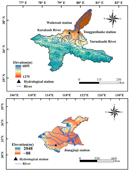
Figure 1.
Overview of the study area.
The monthly runoff data used are from the Wuluwati and Tonguziluoke stations from 1977 to 2013, and the Jiangjiaji station from 1960 to 2000. In total, 80% of the data are used as a training set, 10% as a validation set, and 10% as a testing set.
2.2. Overview of the Hybrid KVMD-KTCN-LSTM-SA Model
In order to reduce the difficulty of predicting monthly runoff, improve the model’s ability of extracting features, and reduce the time of debugging hyperparameters. In this study, a novel KVMD-KTCN-LSTM-SA model is proposed by combining the KOA, KVMD, KTCN-LSTM, and SA mechanism. The proposed model firstly uses KOA combined with VMD to form KVMD. Then, the monthly runoff is decomposed with KVMD to obtain a series of IMFs. After that, the SA mechanism is added to the TCN-LSTM model, and the hyperparameters in this model are optimized by KOA to form the KTCN-LSTM-SA model. This approach improves the ability of the model to extract features and parallel processing. The IMFs are predicted with the KTCN-LSTM-SA model and then the summation of the prediction results is used to attain the final outcomes. The specific processes are as follows (Figure 2):
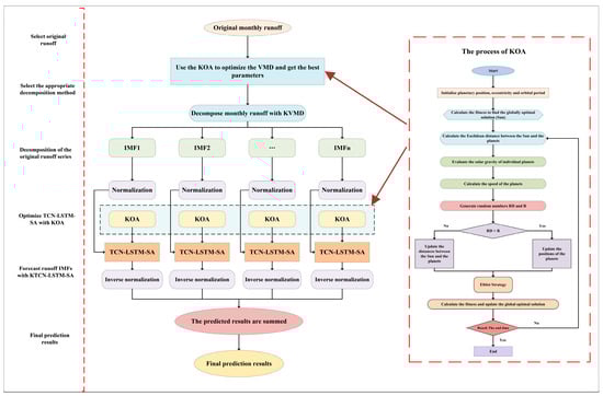
Figure 2.
Schematic structure of the KVMD-KTCN-LSTM-SA model.
Step 1: Select data from three hydrological stations, Tongguziluoke, Wuluwati, and Jiangjiaji.
Step 2: Establish the KOA-VMD algorithm and decompose the monthly runoff data with the KVMD algorithm.
Step 2.1: The initial positions and velocities of the planets are set up to form an initial solution population. The parameters of the KOA are also determined, including the number of planets, gravitational constants, , and so forth. Finally, the fitness function is defined to evaluate the merits of each planet.
Step 2.2: Determine the parameters of the VMD algorithm to be optimized, identify the initial range, and execute the KOA.
Step 2.3: Calculate the fitness of each planet, evaluate the gravitational force of each planet on the other planets, and calculate the combined force vector.
Step 2.4: Update the velocity and position of the planets.
Step 2.5: Repeat steps 2.3 and 2.4 until the termination condition is reached to obtain the optimized VMD parameters.
Step 2.6: Decompose the runoff series with the KVMD.
Step 3: In total, 80% of the data are used as the training set, 10% as the validation set, and 10% as the testing set. The data are normalized with Equation (1), and all values are limited to [0, 1], , , , are the normalized, observed, maximum, and minimum values.
Step 4: Determine the hyperparameters and range of the model to be optimized and use the KOA to optimize the TCN-LSTM-SA model. The optimization process is shown in steps 2.3–2.5.
Step 5: Predict the IMFs with the KTCN-LSTM-SA and sum the runoff component prediction results to obtain the monthly runoff prediction results.
2.3. KVMD-KTCN-LSTM-SA Monthly Runoff Forecasting Model
The KVMD-KTCN-LSTM-SA monthly runoff prediction model proposed in this paper combines the KOA, VMD, TCN-LSTM model, and SA mechanism.
2.3.1. Variational Mode Decomposition (VMD)
Variational mode decomposition, an adaptive decomposition technique, can decompose the signal into a series of intrinsic mode functions (IMFs). VMD decomposes the signal without presetting the window function in advance, and the parameter selection is simple. It overcomes the defects of empirical mode decomposition (EMD), which is prone to modal aliasing and endpoint effect. The runoff series display non-stationary characteristics due to the effects of seasonal rainfall and other factors. Therefore, it is suitable to use VMD. The VMD takes each IMF as an AM-FM signal and sets each constrained modal optimization problem as follows:
represents the set of the K modes, and are the corresponding central frequencies of all IMFs, is the partial derivative of a function with regard to , is the impulse function, and represents convolution.
The augmented Lagrangian is defined as in Equation (3):
represents the punishment parameter, and represents the Lagrange multiplier. Then, the alternate direction method of multipliers (ADMM) algorithm is used to update the IMF and the center frequency of each component . The optimal solution of Equation (3), which corresponds to the saddle point of the unconstrained model, is finally found. The updated equations can be expressed as:
where is the number of iterations, is the noise tolerance, is discrimination accuracy, the mode is the real part of the inverse FT of , , and , representing the Fourier transforms of , and , respectively.
2.3.2. Kepler Optimization Algorithm (KOA)
The Kepler optimization algorithm (KOA) is a novel metaheuristic algorithm inspired by the laws of planetary motion under Kepler’s laws. The positions and velocities of the planets at any given time can be predicted. In KOA, each planet and its position is a candidate solution, which is randomly updated during the optimization process until a termination condition is reached. KOA shows excellent performance in solving complex numerical optimization and machine learning hyperparameter optimization. KOA with the pelican optimization algorithm, slime mold optimization algorithm, and Gray Wolf Optimization Algorithm are tested on CEC2014, CEC2017, CEC2020, and CEC2022 testing sets [31]. KOA shows better performance than the rest of the algorithms. The specific process of KOA is as follows (Figure 3):
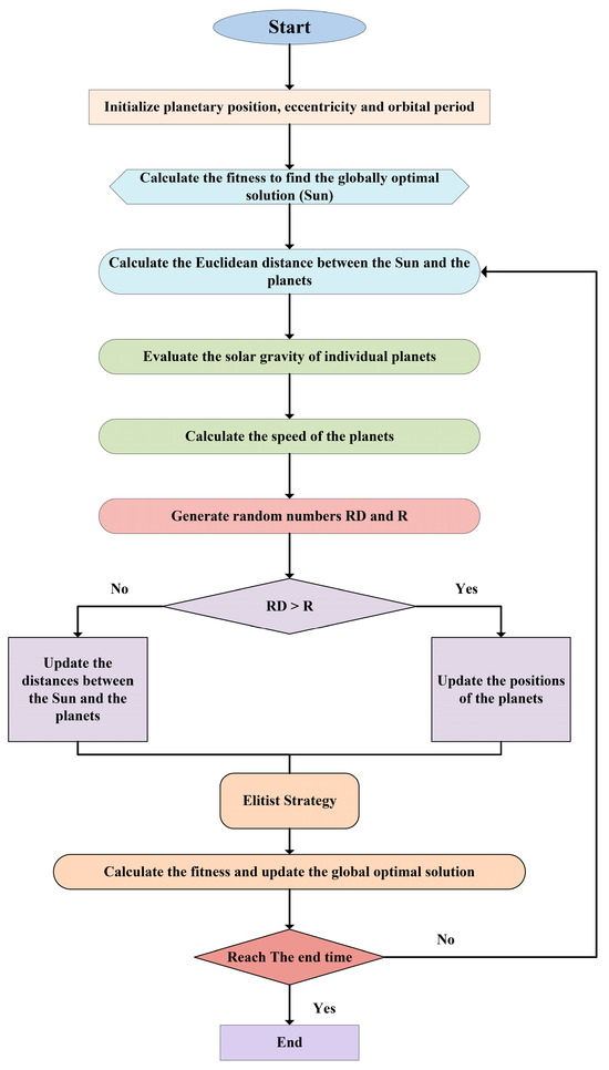
Figure 3.
Flowchart of KOA optimization algorithm.
2.3.3. Temporal Convolutional Network–Long Short-Term Memory–Self-Attention (TCN-LSTM-SA)
The self-attention (SA) mechanism is an important technique in deep learning [32]. The mechanism enables the model to consider information from the entire input sequence instead of relying only on local contextual information. The self-attention mechanism usually consists of three steps: (1) the input sequence is converted into the corresponding vector representation by query, key, and value mapping; (2) the degree of similarity between the query and all the keys is calculated and transformed into a probability distribution by the softmax function; (3) all the value vectors are weighted and summed according to this probability distribution to generate the final output. With the addition of the SA mechanism to TCN-LSTM, it is possible to better capture global dependencies, enhance the selective attention ability of the model, and improve parallelization. The schematic of SA is shown as follows (Figure 4):
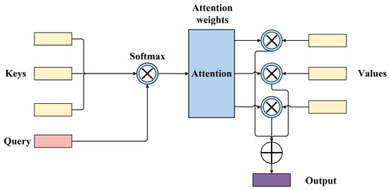
Figure 4.
Structure of the self-attention mechanism.
LSTM has been demonstrated to effectively address the challenges posed by gradient explosion and disappearance that traditional RNN is prone to when dealing with long time sequences [33]. The structure of LSTM mainly consists of the following gates: forget gate, input gate, and output gate. These gate structures cooperate with each other to realize the capture of long-term and short-term dependent information.
TCN combines the parallel processing capability of convolutional neural network (CNN) with the long-term dependent modeling capability of RNN [34]. This method is widely employed in tasks such as time series prediction and sequence classification. TCN is able to effectively capture long time dependencies in time series by introducing causal convolution and dilated convolution. The core idea of TCN is to use convolution operations to extract feature information in time series.
TCN-LSTM connects TCN and LSTM together to process time series. The time series are first input into the TCN, and then causal convolution and dilated convolution are used to extract the multi-scale features of the input [35]. After the features of the time series are extracted by the TCN, the features are passed to the LSTM, which is able to continuously update the hidden state and use its gating mechanism to efficiently deal with dependencies over long time spans. The structure of the TCN-LSTM-SA is shown in Figure 5:
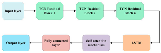
Figure 5.
Structure of the TCN-LSTM-SA model.
2.4. Performance Metrics
To evaluate the prediction ability of the proposed model, the prediction results of the model are evaluated with four evaluation metrics: the Nash–Sutcliffe efficiency coefficient (NSE), the coefficient of determination (R2), the mean absolute error (MAE), and the root mean square error (RMSE).
In the above equations, N is the total number of observations, is the actual value of the daily runoff series, is the corresponding predicted value, is the mean of the actual value, and is the mean of the predicted value.
3. Results
This section presents (1) the decomposition of the monthly runoff series and (2) the specific prediction results of the proposed KVMD-KTCN-LSTM-SA model and the six benchmark models.
3.1. Original and Decomposed Monthly Runoff Series
In this study, monthly runoff series from 1977 to 2013 at the hydrological stations of Tongguziluoke (station A), Wuluwati (station B), and Jiangjiaji (station C) are used. Figure 6 shows the monthly runoff from the three stations; it is evident that the monthly runoff exhibits seasonal fluctuations and is unsteady over the year, which makes accurate prediction very challenging.
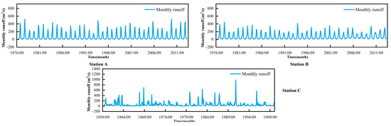
Figure 6.
Monthly runoff series at three stations.
In order to better capture the change pattern of the runoff series and reduce the difficulty of prediction, the runoff series are preprocessed with the KOA-optimized VMD (KVMD). In this case, the parameters of KOA are set as follows: N = 25, = 3, = 0.1, = 15. After optimization, the maximum number of VMD iterations for decomposition at station A is 51 and the number of decomposition layers is 6. The maximum number of VMD iterations for decomposition at station B is 36 and the number of decomposition layers is 6. The maximum number of VMD iterations for decomposition at station C is 33 and the number of decomposition layers is 6. As shown in Figure 7, the monthly runoff series from two stations are decomposed into six components, which are obviously less fluctuating and less complex than the original series. This helps to improve the precision of prediction in the next step.
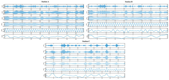
Figure 7.
The runoff subsequences obtained after KVMD of the runoff series from the three stations.
3.2. Prediction Results of the Proposed Model and Six Comparison Models at Three Stations
In the TCN-LSTM-SA model, the KOA is used to optimize four hyperparameters, the number of convolutional kernels, convolutional kernel size, dropout factor, and the number of residual blocks. The number of convolution kernels ranges from 6 to 64, the convolution kernel size ranges from 1 to 10, the residual block ranges from 1 to 10, and the dropout factor ranges from 0.001 to 0.5. In order to demonstrate the prediction performance of the proposed KVMD-KTCN-LSTM-SA (model 7), six benchmark models are selected for comparison: LSTM (model 1), TCN (model 2), TCN-LSTM (model 3), TCN-LSTM-SA (model 4), KTCN-LSTM-SA (model 5), and VMD-TCN-LSTM-SA (model 6). The main hyperparameters of the above models are set as shown in Table 1.

Table 1.
Main hyperparameters setting for different models.
To illustrate the prediction performance of different models more clearly, Table 2 shows the R2, NSE, MAE, and RMSE of the seven models at station A, B, and C. In Table 2, some models show better results in the training and validation periods, but the prediction performance decreases in the testing period. This may be related to the high complexity of the monthly runoff and the low generalization ability of these models. Figure 8, Figure 9 and Figure 10 depict the monthly runoff prediction results of different models. It can be seen that all models can roughly simulate the change patterns of the monthly runoff during the dry season, but when encountering the wet season, some models lack the capability of capturing the runoff peak. When the model predicts excessively variable runoff series, optimization of the model structure and improvement of the model’s ability to capture time series features contribute to the prediction accuracy, such as the combination of different models and the addition of the SA mechanism. In addition, the performance of the hybrid model with the addition of the data preprocessing method shows a significant performance improvement compared to the other models, which is due to the fact that KVMD reduces the range of data fluctuations and reduces the complexity of the runoff series.
Table 2.
Evaluation indexes for three stations.
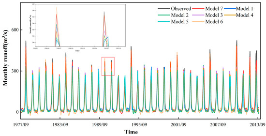
Figure 8.
Runoff prediction results at station A.
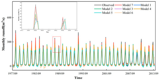
Figure 9.
Runoff prediction results at station B.
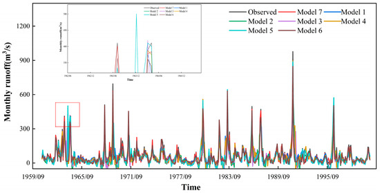
Figure 10.
Runoff prediction results at station C.
4. Discussion
4.1. The Improvement of Model Prediction Performance by SA Mechanism and KOA
Figure 11 shows the box plots of the seven models and the original monthly runoff series in the testing period. It can be seen that the original runoff fluctuates, has more abnormal points, and contains multiple peaks. By combining TCN with models like GRU and BiLSTM, this approach utilizes the excellent parallel processing capability of TCN and the ability of BiLSTM to obtain the contextual linkage of features [36,37]. In addition, SA mechanism could extract internal self-correlation of the training data [38]. Among the models without decomposition, model 4 adds the SA mechanism, in contrast to model 3. This forms TCN-LSTM-SA, which has better predictive ability. The TCN-LSTM-SA model combines the advantages of TCN and LSTM models, which can effectively extract the features and capture the dependencies in the runoff series well. In station A, model 4 has an NSE of 0.773 and an R2 of 0.901 in the testing period, which is higher than the NSE and R2 of models 1, 2, and 3. In station B, model 4 has an NSE of 0.694 and an R2 of 0.802 in the testing period, which is higher than that of models 1, 2, and 3. This indicates that, after the model adds the SA mechanism, it improves the ability of the model to capture the global relationship and enhances the model’s attention to the key parts.
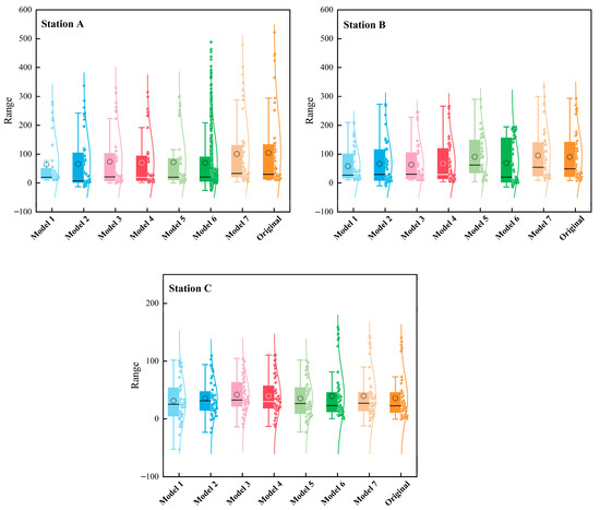
Figure 11.
Box plots of the predictions obtained according to different models during the testing period at three stations.
In monthly runoff prediction with neural networks, the addition of optimization algorithms can effectively improve the model prediction performance [39]. Model 5 adds KOA to model 4 and forms KTCN-LSTM-SA. This model has the structural advantages of model 4 while also obtaining suitable model hyperparameters. It shows that in the testing period of station A, model 5 has a NSE of 0.792 and R2 of 0.914. In the testing period of station B, the NSE of model 5 is 0.727 and R2 is 0.813, which is higher than the other models. It is demonstrated that the KOA improves the performance of the model, avoids the complex hyperparameter selection step, and fully utilizes the capability of the model.
4.2. The Improvement of Model Performance with the Addition of VMD and KVMD
In this paper, six benchmark models and the proposed KVMD-KTCN-LSTM-SA model are used to predict the monthly runoff at stations A and B. From Table 2, it is evident that the prediction models without the decomposition method have a large error in monthly runoff peak prediction. After combining the decomposition method, model 6 and model 7 significantly improve the ability of peak prediction. At station A, model 6 has an NSE of 0.844 and an R2 of 0.853 in the testing period. At station B, model 6 has an NSE of 0.826 and an R2 of 0.842 in the testing period. This indicates that after combining suitable decomposition methods, the prediction difficulty of complex runoff series is reduced effectively. But the parameters of VMD are more difficult to choose. The combination of optimization algorithms to find the best parameters of VMD could effectively improve the prediction accuracy [40,41]. KOA has been shown to be an efficient way to find the optimal parameters. In this research, for the first time, KOA is combined with VMD and TCN-LSTM-SA to form the KVMD-KTCN-LSTM-SA model. This proposed model is able to predict fluctuating time series well and can also be used to predict other time series. Model 7 adds KOA on the base of model 6, and KOA is used to obtain the optimized VMD parameters and model hyperparameters, which makes the prediction results closer to the actual runoff. Model 7 has an NSE of 0.975 and an R2 of 0.986 in the testing period of station A, an NSE of 0.978 and R2 of 0.982 in the testing period of station B, and an NSE of 0.933 and an R2 of 0.947 in the testing period of station C. Among all the models, model 7 achieves the best prediction results, with the lowest MAE and RMSE. This indicates that the prediction model is more consistent with the actual prediction requirements after combining the decomposition method and optimization algorithm.
It is worth noting that model 6 achieves better prediction results in the training and validation periods at station A and B, but the NSE and R2 decrease in the testing period at both stations. This may be due to the fact that there is no optimization algorithm to help the model find the optimal hyperparameters, which makes the model’s predictive performance drop during the testing period. The KVMD-KTCN-LSTM-SA model proposed in this paper combines decomposition methods and optimization algorithms. The model is improved compared to other benchmark models and keeps high prediction performance in the training, validation, and testing periods.
4.3. The Prediction Ability of KVMD-KTCN-LSTM-SA in the Testing Period
In order to demonstrate the prediction ability of different models in the testing period more directly, Figure 12 shows the R2 and NSE at three stations. The proposed model obtains the highest R2 and NSE at station A, station B, and station C. Combined with Table 2, it is shown that both model 6 and model 7 achieved good prediction results in the training and validation periods, but in the testing period, the prediction results of the two models have large differences. This indicates that if the appropriate hyperparameters are not chosen, the prediction results in the testing period are likely to be lower even if better prediction results are obtained in training and validation periods. Based on the prediction results from the three hydrological stations, this proves that the KVMD-KTCN-LSTM-SA model is a model with excellent predictive ability and is suitable for monthly runoff prediction. This contributes to the future management and utilization of water resources. However, the method proposed in this study has not yet taken into account the effects of meteorological factors and human activities on runoff, although it has achieved more satisfactory results at three hydrological stations.
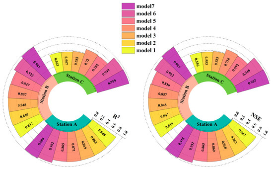
Figure 12.
NSE and R2 at three stations.
5. Conclusions
Monthly runoff prediction is an important research objective for medium- and long-term runoff prediction and is crucial for social planning and economic development. In this study, a KVMD-KTCN-LSTM-SA monthly runoff prediction model is proposed to address the volatility and complexity of monthly runoff series. The model utilizes the data preprocessing method and optimizes the model structure. By predicting the monthly runoff series from 1977 to 2013 at Tongguziluoke and Wuluwati stations, and the monthly runoff series from 1960 to 2000 at Jiangjiaji station, the following conclusions are obtained:
An appropriate data preprocessing method combined with the model can obtain satisfactory monthly runoff prediction results, and the KVMD-KTCN-LSTM-SA model proposed in this study has better prediction performance than the other six benchmark models at three hydrological stations. During the testing period at station A, the R2 is 0.986 and the NSE is 0.975, and during the testing period at station B, the R2 is 0.982 and the NSE is 0.978.
KVMD is vital to the model’s predictive ability. It selects the optimal number of decomposition layers and avoids over-decomposition. This simplifies the difficulty of runoff prediction. In comparison with the model combined with VMD, the model combined with KVMD increases the NSE at stations A, B, and C by 15.52%, 18.40%, and 3.88%, respectively, in the testing period.
The KTCN-LSTM-SA model makes full use of the advantages of different models and improves the parallel capability. This structure of the model can better extract the features of the time series and capture the complex dependencies over long time spans. The model hyperparameters obtained according to the optimization algorithm could effectively improve the prediction accuracy in the testing period. This keeps the prediction performance of the model in the testing period the same as in the training and validation periods.
In this study, the prediction abilities of different models are deeply studied. It is proved that the data preprocessing method combined with the optimization algorithm can effectively improve the performance of the monthly runoff prediction model. This provides a new idea for monthly runoff prediction. However, the influence of meteorological factors is not considered. In future studies, multiple runoff-influencing factors could be combined in the model. In addition, it is also possible to increase the interpretability of the model while improving the prediction accuracy by combining physical hydrological models with machine learning models.
Author Contributions
Conceptualization, S.Z. and K.Z.; methodology, S.Z.; software, S.Z. and C.W.; validation, S.Z. and C.W.; formal analysis, S.Z.; investigation, S.Z.; resources, K.Z.; data curation, K.Z.; writing—original draft preparation, S.Z. and K.Z; writing—review and editing, K.Z.; visualization, S.Z. and C.W.; supervision, K.Z. All authors have read and agreed to the published version of the manuscript.
Funding
This research was supported by the Third Comprehensive Scientific Expedition to Xinjiang (2022xjkk0105), Key research and development project of Xinjiang Autonomous Region (2023B03009-1), and National Natural Science Foundation of China (52279029).
Data Availability Statement
Restrictions apply to the datasets.
Conflicts of Interest
The authors declare no conflicts of interest.
References
- Li, R.; Zhu, G.; Lu, S.; Meng, G.; Chen, L.; Wang, Y.; Huang, E.; Jiao, Y.; Wang, Q. Effects of cascade hydropower stations on hydrologic cycle in Xiying river basin, a runoff in Qilian mountain. J. Hydrol. 2025, 646, 132342. [Google Scholar] [CrossRef]
- Li, R.; Zhu, G.; Lu, S.; Sang, L.; Meng, G.; Chen, L.; Jiao, Y.; Wang, Q. Effects of urbanization on the water cycle in the Shiyang River basin: Based on a stable isotope method. Hydrol. Earth Syst. Sci. 2023, 27, 4437–4452. [Google Scholar] [CrossRef]
- Bárdossy, A.; Anwar, F. Why do our rainfall–runoff models keep underestimating the peak flows? Hydrol. Earth Syst. Sci. 2023, 27, 1987–2000. [Google Scholar] [CrossRef]
- Korsic, S.A.T.; Notarnicola, C.; Quirno, M.U.; Cara, L. Assessing a data-driven approach for monthly runoff prediction in a mountain basin of the Central Andes of Argentina. Environ. Chall. 2023, 10, 100680. [Google Scholar] [CrossRef]
- Le, M.-H.; Kim, H.; Do, H.X.; Beling, P.A.; Lakshmi, V. A framework on utilizing of publicly availability stream gauges datasets and deep learning in estimating monthly basin-scale runoff in ungauged regions. Adv. Water Resour. 2024, 188, 104694. [Google Scholar] [CrossRef]
- Tiwari, D.K.; Kumar, V.; Goyal, A.; Khedher, K.M.; Salem, M.A. Comparative analysis of data driven rainfall-runoff models in the Kolar river basin. Results Eng. 2024, 23, 102682. [Google Scholar] [CrossRef]
- Han, H.; Morrison, R.R. Data-driven approaches for runoff prediction using distributed data. Stoch. Environ. Res. Risk Assess. 2021, 36, 2153–2171. [Google Scholar] [CrossRef]
- Wagena, M.B.; Goering, D.; Collick, A.S.; Bock, E.; Fuka, D.R.; Buda, A.; Easton, Z.M. Comparison of short-term streamflow forecasting using stochastic time series, neural networks, process-based, and Bayesian models. Environ. Modell. Softw. 2020, 126, 104669. [Google Scholar] [CrossRef]
- Adnan, R.M.; Mostafa, R.R.; Elbeltagi, A.; Yaseen, Z.M.; Shahid, S.; Kisi, O. Development of new machine learning model for streamflow prediction: Case studies in Pakistan. Stoch. Environ. Res. Risk Assess. 2021, 36, 999–1033. [Google Scholar] [CrossRef]
- Man, Y.; Yang, Q.; Shao, J.; Wang, G.; Bai, L.; Xue, Y. Enhanced LSTM Model for Daily Runoff Prediction in the Upper Huai River Basin, China. Engineering-Prc. 2023, 24, 229–238. [Google Scholar] [CrossRef]
- Gao, S.; Huang, Y.; Zhang, S.; Han, J.; Wang, G.; Zhang, M.; Lin, Q. Short-term runoff prediction with GRU and LSTM networks without requiring time step optimization during sample generation. J. Hydrol. 2020, 589, 125188. [Google Scholar] [CrossRef]
- Yang, K.; Zhang, X.; Luo, H.; Hou, X.; Lin, Y.; Wu, J.; Yu, L. Predicting energy prices based on a novel hybrid machine learning: Comprehensive study of multi-step price forecasting. Energy 2024, 298, 131321. [Google Scholar] [CrossRef]
- Meng, E.; Huang, S.; Huang, Q.; Fang, W.; Wu, L.; Wang, L. A robust method for non-stationary streamflow prediction based on improved EMD-SVM model. J. Hydrol. 2019, 568, 462–478. [Google Scholar] [CrossRef]
- Yao, Z.; Wang, Z.; Wang, D.; Wu, J.; Chen, L. An ensemble CNN-LSTM and GRU adaptive weighting model based improved sparrow search algorithm for predicting runoff using historical meteorological and runoff data as input. J. Hydrol. 2023, 625, 129977. [Google Scholar] [CrossRef]
- Zhang, X.; Liu, F.; Yin, Q.; Wang, X.; Qi, Y. Daily runoff prediction during flood seasons based on the VMD–HHO–KELM model. Water Sci. Technol. 2023, 88, 468–485. [Google Scholar] [CrossRef]
- Parsaie, A.; Ghasemlounia, R.; Gharehbaghi, A.; Haghiabi, A.; Chadee, A.A.; Nou, M.R.G. Novel hybrid intelligence predictive model based on successive variational mode decomposition algorithm for monthly runoff series. J. Hydrol. 2024, 634, 131041. [Google Scholar] [CrossRef]
- Abdel-Basset, M.; Mohamed, R.; Sallam, K.M.; Alsekait, D.M.; AbdElminaam, D.S. A Kepler optimization algorithm improved using a novel Lévy-Normal mechanism for optimal parameters selection of proton exchange membrane fuel cells: A comparative study. Energy Rep. 2024, 11, 6109–6125. [Google Scholar] [CrossRef]
- Wang, W.-C.; Chau, K.-W.; Qiu, L.; Chen, Y.-B. Improving forecasting accuracy of medium and long-term runoff using artificial neural network based on EEMD decomposition. Environ. Res. 2015, 139, 46–54. [Google Scholar] [CrossRef]
- Zhao, X.; Chen, X.; Xu, Y.; Xi, D.; Zhang, Y.; Zheng, X. An EMD-Based Chaotic Least Squares Support Vector Machine Hybrid Model for Annual Runoff Forecasting. Water 2017, 9, 153. [Google Scholar] [CrossRef]
- Huang, S.; Chang, J.; Huang, Q.; Chen, Y. Monthly streamflow prediction using modified EMD-based support vector machine. J. Hydrol. 2014, 511, 764–775. [Google Scholar] [CrossRef]
- Tan, Q.-F.; Lei, X.-H.; Wang, X.; Wang, H.; Wen, X.; Ji, Y.; Kang, A.-Q. An adaptive middle and long-term runoff forecast model using EEMD-ANN hybrid approach. J. Hydrol. 2018, 567, 767–780. [Google Scholar] [CrossRef]
- Dragomiretskiy, K.; Zosso, D. Variational Mode Decomposition. IEEE Trans. Signal Process. 2014, 62, 531–544. [Google Scholar] [CrossRef]
- Su, T.; Liu, D.; Cui, X.; Dou, X.; Lei, B.; Cheng, X.; Yuan, M.; Chen, R. Prediction of DEDI index for meteorological drought with the VMD-CBiLSTM hybrid model. J. Hydrol. 2024, 641, 131805. [Google Scholar] [CrossRef]
- Xu, Y.; Huang, X.; Zheng, X.; Zeng, Z.; Jin, T. VMD-ATT-LSTM electricity price prediction based on grey wolf optimization algorithm in electricity markets considering renewable energy. Renew. Energy 2024, 236, 121408. [Google Scholar] [CrossRef]
- Krishna Rayi, V.; Mishra, S.P.; Naik, J.; Dash, P.K. Adaptive VMD based optimized deep learning mixed kernel ELM autoencoder for single and multistep wind power forecasting. Energy 2022, 244, 122585. [Google Scholar] [CrossRef]
- Yu, H.; Chen, S.; Chu, Y.; Li, M.; Ding, Y.; Cui, R.; Zhao, X. Self-attention mechanism to enhance the generalizability of data-driven time-series prediction: A case study of intra-hour power forecasting of urban distributed photovoltaic systems. Appl. Energy 2024, 374, 124007. [Google Scholar] [CrossRef]
- Li, J.; Noto, M.; Zhang, Y. Improved Kepler Optimization Algorithm Based on Mixed Strategy. In Advances in Swarm Intelligence; Springer: Singapore, 2024; pp. 157–170. [Google Scholar]
- Zhao, M.; Guo, G.; Fan, L.; Han, L.; Yu, Q.; Wang, Z. Short-term natural gas load forecasting based on EL-VMD-Transformer-ResLSTM. Sci. Rep. 2024, 14, 20343. [Google Scholar]
- Cai, X.; Yuan, B.; Wu, C. An integrated CEEMDAN and TCN-LSTM deep learning framework for forecasting. Int. Rev. Financ. Anal. 2025, 98, 103879. [Google Scholar] [CrossRef]
- Guo, H.; Ling, H.; Xu, H.; Guo, B. Study of suitable oasis scales based on water resource availability in an arid region of China: A case study of Hotan River Basin. Environ. Earth Sci. 2016, 75, 984. [Google Scholar] [CrossRef]
- Abdel-Basset, M.; Mohamed, R.; Azeem, S.A.A.; Jameel, M.; Abouhawwash, M. Kepler optimization algorithm: A new metaheuristic algorithm inspired by Kepler’s laws of planetary motion. Knowl. Based Syst. 2023, 268, 110454. [Google Scholar] [CrossRef]
- Li, W.; Qi, F.; Tang, M.; Yu, Z. Bidirectional LSTM with self-attention mechanism and multi-channel features for sentiment classification. Neurocomputing 2020, 387, 63–77. [Google Scholar] [CrossRef]
- Van Houdt, G.; Mosquera, C.; Nápoles, G. A review on the long short-term memory model. Artif. Intell. Rev. 2020, 53, 5929–5955. [Google Scholar] [CrossRef]
- Xu, Y.; Hu, C.; Wu, Q.; Li, Z.; Jian, S.; Chen, Y. Application of temporal convolutional network for flood forecasting. Hydrol. Res. 2021, 52, 1455–1468. [Google Scholar] [CrossRef]
- Du, J.; Liu, Z.; Dong, W.; Zhang, W.; Miao, Z. A Novel TCN-LSTM Hybrid Model for sEMG-Based Continuous Estimation of Wrist Joint Angles. Sensors 2024, 24, 5631. [Google Scholar] [CrossRef]
- Zheng, J.; Zhang, B.; Ma, J.; Zhang, Q.; Yang, L. A New Model for Remaining Useful Life Prediction Based on NICE and TCN-BiLSTM under Missing Data. Machines 2022, 10, 974. [Google Scholar] [CrossRef]
- Lin, Q.; Yang, Z.; Huang, J.; Deng, J.; Chen, L.; Zhang, Y. A Landslide Displacement Prediction Model Based on the ICEEMDAN Method and the TCN–BiLSTM Combined Neural Network. Water 2023, 15, 4247. [Google Scholar] [CrossRef]
- Yang, W.; Xia, K.; Fan, S. Oil Logging Reservoir Recognition Based on TCN and SA-BiLSTM Deep Learning Method. Eng. Appl. Artif. Intell. 2023, 121, 105950. [Google Scholar] [CrossRef]
- Yue, Z.; Liu, H.; Zhou, H. Monthly Runoff Forecasting Using Particle Swarm Optimization Coupled with Flower Pollination Algorithm-Based Deep Belief Networks: A Case Study in the Yalong River Basin. Water 2023, 15, 2704. [Google Scholar] [CrossRef]
- Wang, W.-C.; Wang, B.; Chau, K.-W.; Zhao, Y.-W.; Zang, H.-F.; Xu, D.-M. Monthly runoff prediction using gated recurrent unit neural network based on variational modal decomposition and optimized by whale optimization algorithm. Environ. Earth Sci. 2024, 83, 72. [Google Scholar] [CrossRef]
- Wen-Chao, B.; Liang-Duo, S.; Liang, C.; Chu-Tian, X. Monthly runoff prediction based on variational modal decomposition combined with the dung beetle optimization algorithm for gated recurrent unit model. Environ. Monit. Assess. 2023, 195, 1538. [Google Scholar] [CrossRef]
Disclaimer/Publisher’s Note: The statements, opinions and data contained in all publications are solely those of the individual author(s) and contributor(s) and not of MDPI and/or the editor(s). MDPI and/or the editor(s) disclaim responsibility for any injury to people or property resulting from any ideas, methods, instructions or products referred to in the content. |
© 2025 by the authors. Licensee MDPI, Basel, Switzerland. This article is an open access article distributed under the terms and conditions of the Creative Commons Attribution (CC BY) license (https://creativecommons.org/licenses/by/4.0/).