Machine Learning-Based Reconstruction and Prediction of Groundwater Time Series in the Allertal, Germany

Abstract

State-of-the-art hydrogeological investigations use transient calibrated numerical flow and transport models for multiple scenario analyses. However, the transient calibration of numerical flow and transport models still requires consistent long-term groundwater time series, which are often not available or contain data gaps, thus reducing the robustness and confidence of the numerical model. This study presents a data-driven approach for the reconstruction and prediction of gaps in a discontinuous groundwater level time series at a monitoring station in the Allertal (Saxony-Anhalt, Germany). Deep Learning and classical machine learning (ML) approaches (artificial neural networks (TensorFlow, PyTorch), the ensemble method (Random Forest), boosting method (eXtreme gradient boosting (XGBoost)), and Multiple Linear Regression) are used. Precipitation and groundwater level time series from two neighboring monitoring stations serve as input data for the prediction and reconstruction. A comparative analysis shows that the input data from one measuring station enable the reconstruction and prediction of the missing groundwater levels with good to satisfactory accuracy. Due to a higher correlation between this station and the station to be predicted, its input data lead to better adapted models than those of the second station. If the time series of the second station are used as model inputs, the results show slightly lower correlations for training, testing and, prediction. All machine learning models show a similar qualitative behavior with lower fluctuations during the hydrological summer months. The successfully reconstructed and predicted time series can be used for transient calibration of numerical flow and transport models in the Allertal (e.g., for the overlying rocks of the Morsleben Nuclear Waste Repository). This could lead to greater acceptance, reliability, and confidence in further numerical studies, potentially addressing the influence of the overburden acting as a barrier to radioactive substances.

1. Introduction

Increasing digitalization due to the development of computing power in recent decades has continuously changed the way of working and the integration of workflows in various disciplines in science and technology, including hydrogeology [1]. Specifically, the possibilities of analyzing and visualizing flow and transport processes on complex numerical grids have advanced considerably by enhanced numerical modeling and GIS methods [2]. Numerical models need a comprehensive database for appropriate calibration and validation for reliable predictions and estimation of uncertainties [3]. These comprehensive databases consist of diverse sources, including remote sensing [4,5], geophysical measurements [4,6,7], climate time series [2], and especially long-term measurements such as groundwater head time series. All of these data require substantial data preparation [3]. The synthesis of these heterogeneous data sources is crucial in order to minimize uncertainty through data integration and subsequent parameterization of the model such that the model error is sufficiently small.

Uncertainties associated with data integration into numerical models arise from a variety of sources, such as parameter estimation, inaccurate remote sensing, geophysical data, or even incomplete groundwater monitoring time series. These can be due to human error [8] during data collection, translation, storage, or inaccurate recording such as defective measuring devices for long-term measurements. Incomplete data can further occur due to the loss of archives or even lack of financial resources [9,10].

Poor and sparse data quality can have a significant influence on modeling accuracy in hydrogeology. These models may result in bad water management decision due to incorrect forecasts of water availability or groundwater pollution. This can lead to additional and unscheduled time and financial requirements for new data recording, recalibration of the transient models, and data analysis. Negative consequences of an inadequate groundwater model calibration are, for example, described in Hunt, Fienen [11]. Based on the Freyberg [12] calibration exercise, the authors describe that even small modifications to the models’ base case can lead to deficiencies that question the ability of the model to make predictions. Such small deficiencies may stem from insufficient data quality.

Therefore, it is essential to provide and ensure accurate and continuous data for numerical modeling. Advanced techniques such as machine learning (ML) can help to close discontinuities in long-term groundwater monitoring time series which likely occur in hydrogeological practice [13,14,15,16,17,18,19,20,21,22,23,24,25,26,27]. The trained ML algorithms (e.g., neural networks, decision trees, and regression models) are able to recognize hydrological patterns (e.g., groundwater head variation) caused by different stresses on the aquifer (e.g., precipitation, evapotranspiration, pumping) [28]. These trained ML algorithms are then able to reconstruct missing values by analyzing the associated input data.

The present study aims at reconstructing and predicting missing groundwater monitoring data at the Bartensleben state-monitoring station in the Allertal (Saxony-Anhalt, Germany) using ML algorithms such as artificial neural networks (TensorFlow, PyTorch), Random Forest, XGBoost and Multiple Linear Regression. The input data consist of monthly precipitation and groundwater head time series from two neighboring stations. Results from the present study in form of the 30-year continuous state monitoring time series will be used for the calibration of a flow and transport model in the Allertal. This numerical model could be used, for example, to predict groundwater head and radionuclide transport using climate scenarios in the context of the decommissioning of the Morsleben Nuclear Waste Repository. Figure 1 visualizes the structure and the main aims of the present paper.

2. Site Description and Explorative Data Analysis (EDA)

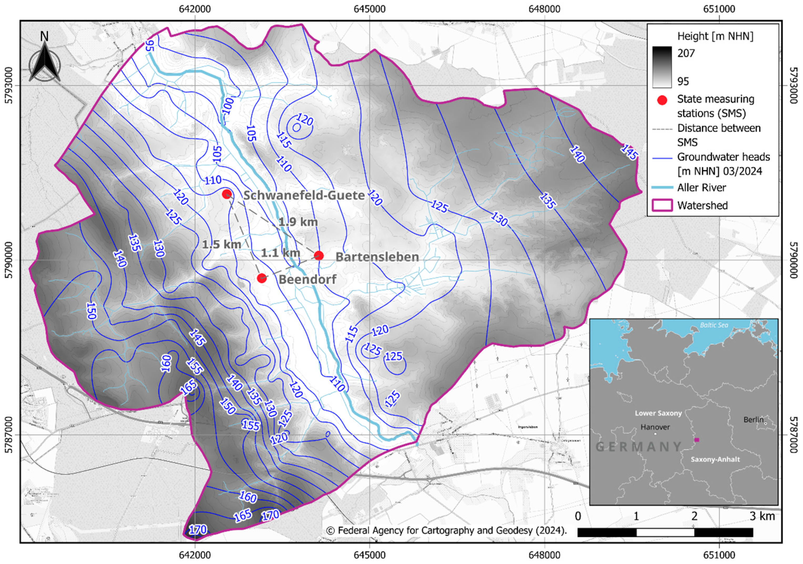
2.1. Study Area and Data Preprocessing

The underlying data consist of precipitation and groundwater monitoring time series for the three state stations: Bartensleben (BART), Beendorf (BEEN) and Schwanefeld-Güte (SWG). All stations are located within the Allertal, situated in Saxony-Anhalt, Germany, shown in Figure 2. The groundwater time series are publicly freely available data and can be downloaded from the website of the State Authority for Flood Protection and Water Management of Saxony-Anhalt [29]. Continuous time series of groundwater potentials are available for the shallow groundwater state-monitoring stations on a daily or weekly basis. General information about the data is provided in (

Table 1. Key attributes of the groundwater monitoring data from the three state-monitoring stations, Bartensleben (BART), Beendorf (BEEN), Schwanefeld-Güte (SWG), considered in the present study.

Monitoring Name	BART	BEEN	SWG
Time Period—Start	November 1997	November 1994	November 1994
Time Period—End	May 2024	May 2024	May 2024
Monitoring Type	GW-monitoring tube	GW-monitoring tube	GW-monitoring tube
Easting	644125	643147	642547
Northing	5790076	5789689	5791133
Monitoring Interval	Daily	Weekly	Weekly
Unit	m	M	m
Base [m]	9	5	31
Measuring Point [m]	122.05	115.84	122.54
Groundwater Body	Upper Aller Mesozoic bedrock on the right	Upper Aller Mesozoic bedrock on the left	Upper Aller Mesozoic bedrock on the left

). Groundwater potential is originally given as the distance between the reference measurement height of the well and the groundwater level depth to groundwater $\Delta G$ [m] (also known as tap). While $\Delta G$ for the stations BEEN and SWG cover an overlapping period, starting from November 1994, $\Delta G_{BART}$ for BART started with a delay of 3 years in November 1997. All time series ended in May 2024. The $\Delta G$ time series were imported into a SQL database and exported via SQL queries to a Jupyter Notebook [30] for further processing. To ensure consistency for precipitation and groundwater data, both datasets were aggregated and synchronized from their respective temporal resolutions—daily (groundwater), weekly (groundwater), or monthly (precipitation)—into a monthly average time series due to the limiting availability of monthly precipitation. $\Delta G$ was further processed, converted, and scaled into monthly observed groundwater head differences $\Delta H_{obs}$ [mm], where the units were chosen to ensure consistency with precipitation. $\Delta H_{obs}$ was chosen as groundwater potential data, in accordance with Li, Yang [31], who studied hydrological time series and found out that water level at previous time steps are critical for the forecasting of the present water level. Consequently, $\Delta H_{obs}$ directly quantifies the monthly change in groundwater head.

Precipitation data ($P$) are freely available data from the Climate Data Center [32]. The data are available as spatial rasters of monthly precipitation in mm with a spatial resolution of 1 × 1 km for each month since 1881 for Germany. The original provided dataset contains 392,965 raster cells representing P data over a period of 142 years until May 2024 (

Table 2. Attributes of precipitation data (P) from the three state-monitoring stations, Bartensleben (BART), Beendorf (BEEN), and Schwanefeld-Güte (SWG), considered in the present study.

Monitoring Name	BART	BEEN	SWG
Time Period—Start	January 1881	January 1881	January 1881
Time Period—End	May 2024	May 2024	May 2024
Interpolation Type	Inverse-distance, raster type	Inverse-distance, raster type	Inverse-distance, raster type
Unit	mm	Mm	mm

).

In order to generate three synchronized precipitation time series corresponding to the $\Delta H_{obs}$ time series of BART, BEEN, and SWG, the precipitation raster dataset was preprocessed using Quantum Geographic Information System (version 3.28.10) [33]. A PyQGIS script [34] was developed to spatially reduce the German-wide single monthly precipitation raster dataset with a temporal resolution of 142 years to the monitoring stations. The reduced but temporarily unconnected data were then temporally processed to create a continuous time series for each monitoring station. Finally, each precipitation time series was then synchronized to the corresponding $\Delta H_{obs}$ time series length (November 1994–May 2024) of each monitoring station as shown in Table 1.

2.2. Explorative Data Analysis (EDA)

Figure 3 and

Table 3. Statistical summary of the (a) groundwater head differences $∆H_{obs}$ [mm] and (b) precipitation [mm] for the three state-monitoring stations, Bartensleben (BART), Beendorf (BEEN), and Schwanefeld-Güte (SWG), considered in the present study.

Data Statistics	$\left(\mathbf{a}\right) ∆{\mathit{H}}_{\mathit{o}\mathit{b}\mathit{s}}$ [mm]			(b) Precipitation [mm]
Monitoring Name	BART	BEEN	SWG	BART	BEEN	SWG
Count	316	355	355	355	355	355
Mean	−0.22	−0.29	0.2	47	49	49
Std.	57	31	168	26	27	27
Min	−193	−103	−433	1	1	1
10%	−58	−33	−175	19	19	19
25%	−35	−20	−83	29	30	30
50%	−10	−5	−38	42	45	44
75%	26	15	54	63	65	66
90%	73	38	237	80	83	83
Max	263	133	678	145	153	156

describe univariate statistical parameters, such as the number of measurements, mean, minima, maxima, and quantiles for (a) $\Delta H_{obs}$ and (b) $P$ for the three locations considered in the present study. BEEN and SWG have the same number of $\Delta H_{obs}$ observations (355), while BART has 316 $\Delta H_{obs}$ observations.

$\Delta H_{obs}^{SWG}$ (121.56 m.a.s.l.) is characterized by the highest mean and standard deviation in 0.2 ± 168 mm (Figure 3a and Table 3a), indicating higher significant fluctuations compared to the other two groundwater monitoring stations, while $\Delta H_{obs}^{BEEN}$ (115.84 m.a.s.l.) has the lowest mean and standard deviation of −0.29 ± 31 mm. The percentiles of $\Delta H_{obs}^{BART}$ (121.25 m.a.s.l.) with mean and standard deviation in (−0.22 ± 57 mm) and $\Delta H_{obs}^{BEEN}$ are closer to each other, suggesting variations that are more moderate. Furthermore, $\Delta H_{obs}^{SWG}$ is characterized by the larger groundwater level fluctuations in both directions, indicating potential outliers or climatic conditions significantly affecting the groundwater head conditions.

All three monitoring stations have an equal number of monthly observations for $P$ (count = 355) due to adaption to the maximum length of the $\Delta H_{obs}$ time series. Figure 3b and Table 3b show that the three locations have very similar average monthly precipitation values and standard variations between 4749 ± 26–27 mm, indicating similar variability. All sites have the same minimum precipitation value (1 mm).

Overall, the analysis reveals that $\Delta H_{obs}^{SWG}$ exhibits the highest variability and extreme values, while $\Delta H_{obs}^{BEEN}$ shows the least variability. Hence, $\Delta H_{obs}^{BART}$ ranges between $\Delta H_{obs}^{SWG}$ and $\Delta H_{obs}^{BEEN}$. In terms of $P$, all three sites are quite similar according to their statistical properties due to similar precipitation patterns and close proximity.

Figure 4 presents the correlation matrix for $\Delta H_{obs}$ and $P$ measured at the groundwater state-monitoring stations BART, BEEN, and SWG. Values close to 1 (dark red color) indicate a strong positive correlation, while values close to 0 (dark blue color) indicate a weaker correlation. Values close to 0 (white color) indicate that there is no linear correlation between the variables. P at all stations is perfectly correlated (1) with each other, indicating again that the precipitation patterns across BART, BEEN, and SWG are similar. This supports findings from Pang, Zhang [35], who describe that, on a monthly temporal scale, precipitation measurements from different datasets exhibit similar temporal records. Generally, the correlation coefficients for $\Delta H_{obs}^{BART}$ and $P$ for all stations indicate a weak positive linear relationship. However, a positive correlation suggests that, as P increases, the $\Delta H_{obs}^{BART}$ also tends to increase at both sites. The correlation coefficients of $\Delta H_{obs}^{BART}$ to $\Delta H_{obs}^{SWG}$ (0.75), $\Delta H_{obs}^{BART}$ to $\Delta H_{obs}^{BEEN}$ (0.49), and $\Delta H_{obs}^{BEEN}$ to $\Delta H_{obs}^{SWG}$ (0.47) indicate strong to moderate positive correlations, respectively. This suggests that concurrent changes in $\Delta H_{obs}^{BART}$ and $\Delta H_{obs}^{SWG}$ are stronger correlated than corresponding changes in $\Delta H_{obs}^{BART}$ and $\Delta H_{obs}^{BEEN}$. Overall, across all stations, there is a generally positive correlation between $P$ and $\Delta H_{obs}$. This indicates that precipitation directly influences groundwater dynamics, although the intensity of this impact varies. Therefore, in the present study, it is assumed that precipitation is the dominant factor that represents the climatic conditions that influence the groundwater level variations. While evaporation or filter depth are neglected here in addition to precipitation for the reason mentioned above, these can in principle be included, similar to the approach of Wunsch, Liesch [36], whereby temperature data could be added to the input dataset as a proxy for evaporation. Figure 5 illustrates the approx. 30-year time series, for the observed groundwater head differences ΔH_obs and precipitation P. The data span from November 1994 to May 2024 and includes observations from (a) BART, (b) BEEN, (c) SWG, and (d) that show each time series, respectively, overlapped into one figure. Positive $\Delta H_{obs}$ values denote an increase in groundwater head compared to the previous month, whereas negative values represent a decrease in groundwater head.

The time series for $\Delta H_{obs}^{BART}$ started with a 3-year delay in November 1997, as indicated by the first dashed vertical line in Figure 5a. The data show alternating periods of increase and decrease in $\Delta H_{obs}^{BART}$, reflecting a dynamic groundwater system. Notable positive peaks were observed during the winter months, specifically in February 1999 (150 mm), January 2008 (262.5 mm), and January 2011 (237.5 mm), indicating extreme values in the form of significant increases in $\Delta H_{obs}^{BART}$. Conversely, notable negative peaks occurred during the summer periods like May 2008 (−192.5 mm), June 2010 (−140 mm), and June 2013 (−140 mm), showing significant decreases.

The time series for $\Delta H_{obs}^{BEEN}$ and $\Delta H_{obs}^{SWG}$ are visualized in Figure 5b and c, respectively. $\Delta H_{obs}^{BEEN}$ shows significant positive peaks during the winter months of early 2000, particularly in January 2004/2005 (82.5 mm), December 2017 (132.5 mm), and March 2023 (112.5 mm). In contrast, $\Delta H_{obs}^{SWG}$ shows more extreme fluctuations, with notable positive peaks in November 2002 (677.5 mm) and January 2012 (612.5 mm).

Both time series for $\Delta H_{obs}^{BEEN}$ and $\Delta H_{obs}^{SWG}$ feature several periods of significant decreases in the summer months. For $\Delta H_{obs}^{BEEN}$, these include June 2006 (−72.5 mm), June 2018 (−67.5 mm), and April 2023 (−102.5 mm). $\Delta H_{obs }^{SWG}$ shows significant decreases in May 1995 (−432.5 mm), September 2002 (−405 mm), and June 2010 (−347.5 mm). The $\Delta H_{obs}^{BART}$ time series lies between $\Delta H_{obs}^{BEEN}$ and $\Delta H_{obs}^{SWG}$ when comparing all positive and negative peaks. Overall, the explorative data analysis reveals that the $\Delta H_{obs}^{BART}$ time series shows similar seasonal trends as $\Delta H_{obs}^{BEEN}$ and $\Delta H_{obs}^{SWG}$, with positive winter peaks and negative summer peaks. Qualitatively, the peak positions between $\Delta H_{obs}^{BART}$ and $\Delta H_{obs}^{SWG}$ are more consistent than those between $\Delta H_{obs}^{BART}$ and $\Delta H_{obs}^{BEEN}$, supporting the greater correlation between $\Delta H_{obs}^{BART}$ and $\Delta H_{obs}^{SWG}$ established above.

Given the similarity in seasonal patterns and the intermediate magnitude of fluctuations, the time series data from $\Delta H_{obs}^{BEEN}$ and $\Delta H_{obs}^{SWG}$ can be used to reconstruct the missing groundwater head dynamics in $\Delta H_{obs}^{BART}$. The consistent seasonal trends across these locations support the reliability of using data from $\Delta H_{obs}^{BEEN}$ and $\Delta H_{obs}^{SWG}$ as proxies for understanding and predicting groundwater behavior in $\Delta H_{obs}^{BART}$.

3. Machine Learning (ML) Methods and Workflow

According to Sahour, Gholami [37], ML-based models are able to recognize data patterns and interparameter dependencies. Therefore, this chapter addresses ML supervised learning approaches instead of unsupervised learning. The focus lies on key frameworks and hyperparameters for model development and implementation used in the present study. In general, supervised-learning algorithms learn from labeled training data, while unsupervised learning require unlabeled data. Labeled data consist of an input–output pair in order to learn a function that maps the given inputs to the corresponding outputs, while unsupervised learning uses unlabeled data to find patterns or structures on their own. In this study, labeled data are available, such as $P$ of the reference and missing value monitoring stations as well as $∆H_{obs}$ of the reference monitoring station (BEEN or SWG) as inputs. Only during model training and testing is the input–output pair completed by the corresponding output $∆H_{obs}$ of the missing value monitoring station for training and comparison. In the following, different algorithms for supervised-learning are presented.

TensorFlow [38] and PyTorch [39], two powerful Deep Learning libraries offering flexible and scalable solutions. Followed by classical machine learning algorithms, such as Random Forests and XGBoost, which are particularly suited for structured data analysis. Finally, the chapter covers Multiple Linear Regression, a fundamental method for predicting continuous target variables.

Hyperparameters are configuration settings used to control the behavior of ML algorithms. Hyperparameters are set before training begins and are not updated during training, unlike model parameters such as the weights in a neural network. They play a critical role in the performance and efficiency of ML models [40,41,42]. Overall, these ML tools and techniques provide the basis for the development of accurate and robust models for the reconstruction and prediction of the continuous groundwater head time series [43].

By integrating Deep Learning frameworks with traditional machine learning algorithms, the above mentioned advantages of both methods are combined, such that a model ensemble offers flexible and scalable solutions that are particularly suited for data analysis. This in-depth analysis helps specify bandwidths consisting of results of the different models for evaluating reconstructed and predicted groundwater head time series, while minimizing the risk of overfitting.

3.1. Deep Learning Frameworks—Artificial Neural Network

3.1.1. TensorFlow

TensorFlow [38] is an open-source library for machine learning developed by the Google Brain team Abadi, Barham [44]. It provides tools for operating machine learning systems on large datasets with a high degree of flexibility [45], enabling experimental model development and user-friendly parameter control, especially when integrated into the Keras application programming interface [46]. TensorFlow is used in numerous groundwater-related applications (e.g., [20,47,48]). In the present study, version 2.12.0 of TensorFlow interfaced with Keras was used to build an artificial neural network (ANN) model. Specifically, a feed forward neural network [49] was generated. In this type of neural network, an input value is given into the first neuron. This generates an output that, while changing its value within each neuron, propagates through a series of neurons. Within the neural network, a neuron within a certain layer receives the output value of the previous layer as an input value. Finally, that value reaches the outermost neuron, which gives the final output. The number of layers and the number of neurons within a layer is called the topology of a neural network [50]. The mathematical model of a single neuron originates in the McCulloch and Pitts [51] neuron. Mathematically, the output $y_i$ of a single neuron $j$ is defined as

$$y_j=f \left({\sum }_{j=1}^m\left(w_{ij}{y}_i+b_i\right) \right),$$

(1)

where $f$ is the activation function, m is the number of inputs into the jth neuron, $w_{ij}$ is the weight, $y_i$ is the output of the previous neuron, and $b_i$ is the bias. Information about these terms is given in

Table 4. Best-fit hyperparameter set for the state-monitoring station Beendorf (BEEN).

Hyperparameter	TensorFlow	PyTorch	Random Forest Regression	XGBoost	Multiple Linear Regression
Learning Rate	0.01	0.001		0.1
Number of Epochs	1000	10
Optimizer	Adamax	Adam
Activation Functions	ReLu	ReLu
Number of Layers and Units per Layer	2	2
Neurons	3:250:1950:1	3:1050:256:1
Loss Function	MSE	MSE
Dropout Rate	0.4
Number of Trees (n_estimators)			10	8
Maximum Depth (max_depth)			5	3
Minimum Samples per Leaf (min_samples_leaf)			1
Minimum Samples to Split (min_samples_split)			2
Criterion (criterion)			Squared error	Squared error
${\epsilon }_{constant}$					−10.174
$P_{constant}^{BEEN}$ [mm]					12.234
$P_{constant}^{BART}$ [mm]					−12.512
$\Delta H_{constant}^{BEEN}$ [mm]					0.797

and

Table 5. Best-fit hyperparameter set for the state-monitoring station Schwanefeld-Güte (SWG).

Hyperparameter	TensorFlow	PyTorch	Random Forest Regression	XGBoost	Multiple Linear Regression
Learning Rate	0.01	0.001		0.1
Number of Epochs	1000	1000
Optimizer	Adamax	Adam
Activation Functions	ReLu	ReLu
Number of Layers and Units per Layer	2	2
Neurons	3:750:1850:1	3:256:8:1
Loss Function	MSE	MSE
Dropout Rate	0.4
Number of Trees (n_estimators)			4	100
Maximum Depth (max_depth)			10	6
Minimum Samples per Leaf (min_samples_leaf)			2
Minimum Samples to Split (min_samples_split)			10
Criterion (criterion)			Squared error	Squared error
${\epsilon }_{constant}$					−5.218
$P_{constant}^{SWG}$ [mm]					1.128
$P_{constant}^{BART}$ [mm]					−1.071
$\Delta H_{constant}^{SWG}$ [mm]					0.280

. By iteratively adjusting the weights, a neuronal network can be optimized until its output matches some target values. That process in combination with a result evaluation within each iteration is called training and testing. By employing the growing algorithm after Berkhahn, Fuchs [50], the best-fit topology was found. Further a random search of significant hyperparameters was performed to find an appropriate hyperparameter combination. The hyperparameters were varied, namely learning rate, number of epochs, optimizer, activation function, loss function, and the presence of a dropout layer with a specific dropout rate. The best-fit combinations of all the hyperparameters are listed in Table 4 and Table 5.

3.1.2. PyTorch

PyTorch [39] is another popular open-source machine learning library developed by Facebook. Unlike TensorFlow, PyTorch uses dynamic computation graphs, which means that the graphs can be modified during runtime. This feature, and its internal use of NumPy [52], makes PyTorch powerful when handling large arrays and useful for research and experimental applications. This has been used in numerous hydrology-related applications [22,53,54,55]. In the present study, PyTorch (version. 2.3.1) is used in order to calculate simulated $\Delta H_{sim}^{BART}$ values and compare them to actual observed $\Delta H_{obs}^{BART}$. The typical PyTorch workflow starts with data preparation, including scaling between 0 and 1, for the multidimensional arrays (Tensors) used in PyTorch. This is followed by the model development and hyperparameter selection of the neural network, consisting of multiple linear layers (here, two layers). Then, the forward calculations including the ReLU activation function are initiated, generating the output, and compared to the observed data using the Mean Squared Error (MSE) as the loss function. The model is able to learn non-linearity due to the ReLu function and tends to show better convergence performance than tanh or sigmoid functions [17,56]. PyTorch uses an automatic differentiation system called Autograd, enabling the automatic calculation of the parameter gradients. The weights of the neurons are optimized using an optimizing algorithm (here, Adam). The training is repeated several times (called epochs) while optimizing the model. Multiple ranges of each hyperparameter were executed. The best-fit hyperparameters for PyTorch used in the present study are shown in Table 4 and Table 5.

3.2. Classical Machine Learning Algorithms

3.2.1. Random Forest Regression

Random Forest Regression is a powerful and versatile ML technique for predicting continuous values [57]. The algorithm is based on the bagging principle, meaning that multiple decision trees are trained at once and combined by using the average for robust and accurate prediction [58]. A decision tree splits the data into subsets based on feature conditions [59], creating a tree-like structure. Each internal node represents a decision based on a feature, and each leaf node gives the final prediction (here, a value due to the regression analysis). The model aims at splitting the data, resulting in a maximized purity or minimized error within each subset, making it easy to interpret. However, decision trees can overfit the data [60,61], such that the Random Forest Regression uses an ensemble approach in which a number of trees are trained on different subsets of the data, resulting in reduced overfitting. Random Forest is relatively robust to outliers and performs well across a wide range of data types, making it a popular choice in various application areas, such as financial analysis, healthcare, and environmental modeling. Random Forest has been used in numerous hydrology-related applications [18,21,62,63,64,65]. Random Forest models are found to be less sensitive to reductions in sample size [66]. Hence, for applications with few data, Random Forest models are advantageous. In recent years, the most popular ML method for groundwater level prediction is Random Forest, followed by support vector machines and the ANN [67]. Therefore, in this study, Random Forest (scikit-learn package, version. 1.2.2, [68]) is used in order to calculate simulated $\Delta H_{sim}^{BART}$ values and compare them to actual observed $\Delta H_{obs}^{BART}$. The data processing steps are similar to those of the Deep Learning Methods and are described in Section 2.1. The hyperparameters used for the Random Forest Regression are n estimators, max depth, min samples split, and min samples leaf. A descriptive definition of hyperparameters can be found in the Appendix A Table A1. The best-fit Random Forest Regression hyperparameters used in the present study are shown in Table 4 and Table 5.

3.2.2. XGBoost (eXtreme Gradient Boosting)

XGBoost (eXtreme Gradient Boosting) is a highly efficient and flexible ML algorithm that has become a popular choice for both classification and regression tasks. Chen and Guestrin [69] introduced and combined weak learners (usually simple decision trees) to create a strong predictive model. The advantage of XGBoost lies in the objective function, which minimizes the loss function (e.g., Mean Squared Error) and therefore the residuals of the weakest learners, instead of adjusting new weights after each training. Each new tree corrects the errors made by the previous ones, improving the overall model performance iteratively. XGBoost is used in numerous practical applications across industries, from finance to healthcare to groundwater (e.g., [70,71]). XGBoost has been used in numerous hydrology-related applications [24,72,73,74,75]. The hyperparameters used for the XGBoost are n estimators, max depth, and the loss function. A definition of hyperparameters can be found in Appendix A Table A1. In the present study, the XGBoost library (version 2.1.0.) was applied for XGBoost and the best-fit XGBoost hyperparameters are shown in Table 4 and Table 5.

3.2.3. Multiple Linear Regression (MLR)

In machine learning, Multiple Linear Regression (MLR) is a statistical technique [76] that is used to model the linear relationship between dependent and multiple independent variables, enabling quantification and prediction of complex hydrological processes. MLR was used in multiple hydrological applications, such as Hodgson [13], Jobson [14], Sahoo and Jha [16], Fathian [19], Ehteram and Banadkooki [23], and Seelbach, Hinz [77]. The typical model equation can be expressed as follows [14]:

$$y={\beta }_0+{\beta }_1{X}_1+\cdots +{\beta }_n{X}_n+\epsilon ,$$

(2)

where

y = predicted value based on the independent variables;

${\beta }_0$ = value of y, when all other $\beta$ parameters are set to 0;

${\beta }_1{X}_1$ = the regression coefficient ${\beta }_1$ of the first independent variable $X_1$;

${\beta }_n{X}_n$ = the regression coefficient ${\beta }_n$ of the nth independent variable $X_n$.

The coefficients are parameters that control the learning process of the model. In the present study, the statsmodel api (version 0.14.0) was applied for MLR. Table 4 and Table 5 includes the Multiple Linear Regression coefficients used in the present study.

3.3. Performance Metrics

To evaluate and compare the performance of machine learning (ML) models, it is essential to use metrics that provide insight into their accuracy and reliability and to select models based on their overall performance across different metrics [78]. Commonly used performance metrics for model optimization and assessment are the Mean Squared Error (MSE), Mean Absolute Error (MAE), and the Nash–Sutcliffe Efficiency (NSE), among others [79,80]. These metrics quantify average errors and their variance thus providing different perspectives on model performance. Understanding and applying these metrics is essential for improving models while ensuring robust and accurate model applications, while each metric can reveal different information about individual models [80]. All performance metrics are applied to each ML method used in the present study (artificial neuronal network (TensorFlow, PyTorch), Random Forest, XGBoost, and Multiple Linear Regression). Detailed information about each performance metric can be found in the appendix.

3.4. Workflow

This subsection describes the workflow used in the present study, consisting firstly of model development (Step 1) training and (Step 2) testing and evaluation), and secondly model application ((Step 3) reconstruction and (Step 4) prediction of the simulated groundwater differences $\Delta H_{sim}^{BART}$), where Step 3 and Step 4 are the main aims of the current study.

Figure 6 describes the workflow. The first column describes the input vector $X_{obs,\ast }$, which includes the time series of the observed precipitation $P$ and groundwater differences $\Delta H_{obs}$ of BEEN or SWG and of BART, the last column describes $y_{sim,\ast }$, which is the simulated, reconstructed, or predicted $\Delta H_{sim}^{BART}$ by each selected ML model. According to Faridatul [81], precipitation is the primary source of groundwater recharge. In this study, precipitation is used as the only stress parameter affecting the aquifer. This assumption was also made for practical reasons because it simplifies the development of the ML models. In further studies, the ML models could be trained and tested with an input dataset covering more stress parameters, such as evapotranspiration or air temperature. However, the same data resolution of the input parameters as presented in this study is required.

In the present study, prior to training and testing, a random sampling of the data was performed in addition to data separation. By trying out different split sizes of the training and test dataset followed by training and testing of the ANN model, it was found that a split into 70% training data and 30% test data leads to a convergence of the NSE as evaluation metric (Figure A1). This split agrees with results from Seidu, Ewusi [26] and Ali, Awwad [82]. In the Appendix A (Figure A2 and Figure A3), the random selection of data points for precipitation and $\Delta H_{obs}$ are shown, where the lighter color refers to data used for training and a darker color is used for testing. After splitting, the data were scaled and back scaled between 0 and 1 during model development and application to account for numerical stability during weight adjustment prior to the start of training. After each model run and back transformation, performance metrics were calculated, compared, and evaluated against the observations.

For each ML method, numerous combinations (>3000 combinations, each) and bandwidth of hyperparameters were tested, compared, and evaluated during training, testing, and prediction, using MSE, MAE, and NSE as performance metrics.

According to the qualitative classification of NSE values from Moriasi, Gitau [83], a model performance was defined to be “satisfactory” for NSE > 0.5. Therefore, for each ML model and its multiple hyperparameter combinations, a list was generated covering all performance metrics. These lists were then sorted according to the performance metrics, followed by the manual selection of the single best performing model. Comparing the performance metrics of each model against both the training and test datasets was part of the manual selection process. If both metrics showed a large discrepancy (e.g., NSE_train = 0.91, NSE_test = 0.4), it was discarded due to overfitting of the trained model. The optimal model is selected by the metrics that show the best performance on the training and test datasets with the least discrepancy. Table 4 and Table 5 show the hyperparameters with the best fit for each ML model based on BEEN and SWG, respectively.

After successful model training, testing, and evaluation, the second part is the model application, where in (Step 3) missing groundwater head differences $\Delta H_{sim}^{BART}$ were reconstructed for the period November 1994 to November 1997 and (Step 4) predicted $\Delta H_{sim}^{BART}$ for the period January 2023–May 2024, followed by a comparison to the observed $\Delta H_{obs}^{BART}$ data.

4. Results

4.1. Training and Testing

Figure 7 and Figure 8 show the time series of observed compared to simulated $\Delta H^{BART}$ from November 1997 to December 2022. In (a), the ML ensembles and all simulated time series $\Delta H_{sim}^{BART}$ are shown, followed by all simulated time series separated in the (b) Deep Learning Methods (TensorFlow and PyTorch), (c) tree-based methods (Random Forest and XGBoost), and (d) the Multiple Linear Regression for BART based on input data from both BEEN and SWG, respectively. Each ML model based on BEEN (ML_BEEN) and SWG (ML_SWG) fits well during the hydrological summer from May to Oct. The mean $\Delta H_{sim}^{BART}$ of all ML_BEEN models show −8 ± 25 mm (

Table 6. Statistical analysis of hydrological summer machine learning values $\Delta H_{sim}^{BART}$ compared to observed values for Beendorf (BEEN) $\Delta H_{sim}^{BART}$.

May–October BEEN	TensorFlow	PyTorch	Random Forest Regression	XGBoost	Multiple Linear Regression	Observed
count	175	175	175	175	175	157
mean	−10	0	−12	−6	−14	−27
std	29	24	28	16	28	36
min	−124	−38	−120	−54	−100	−193
25%	−23	−18	−23	−7	−31	−48
50%	−8	−5	−15	−7	−15	−25
75%	5	12	−3	−4	−1	−5
max	53	80	108	60	87	108

), while the mean of all ML_SWG models show −17 ± 24 mm (

Table 7. Statistical analysis of hydrological summer machine learning values $\Delta H_{sim}^{BART}$ compared to observed values for Schwanefeld-Güte (SWG) $\Delta H_{obs}^{BART}$.

May–October SWG	TensorFlow	PyTorch	Random Forest Regression	XGBoost	Multiple Linear Regression	Observed
count	175	175	175	175	175	157
mean	−16	−18	−18	−12	−21	−27
std	24	24	28	17	28	36
min	−136	−114	−116	−74	−123	−193
25%	−25	−30	−34	−21	−29	−48
50%	−14	−20	−18	−16	−18	−25
75%	−4	−9	−1	−2	−12	−5
max	68	82	113	60	135	108

). For comparison, the observed $\Delta H_{obs}^{BART}$ show −27 ± 36 mm. During the hydrological winter, only the mean $\Delta H_{sim}^{BART}$ of all ML_SWG models fit well (24 ± 53 mm) to the observed $\Delta H_{obs}^{BART}$ (34 ± 65 mm). All ML_BEEN models underestimated the observed data (9 ± 33 mm). Further, all applied ML models underestimated the extreme peaks during the hydrological winter (e.g., January 2008, May 2008, March 2010, or January 2011), indicating that extreme events occurring during the hydrological winter are not well covered by the ML models, compared to the well-captured hydrological summer.

Figure 9 and Figure 10 show the observed to simulated plots for each ML model. The plotted data are colored according to the absolute residuals of observed $\Delta H_{obs}^{BART}$ and simulated $\Delta H_{sim}^{BART}$. Most of the data surround the 1:1 perfect fit line. The training and test NSEs, shown in

Table 8. Assessment of machine learning model performance via MSE, MAE, and NSE metrics for state-monitoring station Schwanefeld-Güte (SWG).

Phase	TensorFlow	PyTorch	Random Forest Regression	XGBoost	Multiple Linear Regression
TRAIN
MSE	732.43	1064.59	689.06	1116.30	1312.28
MAE	18.69	23.86	19.16	24.00	26.44
NSE	0.71	0.70	0.81	0.69	0.64
TEST
MSE	1412.91	1452.25	1389.62	1489.22	1523.56
MAE	28.18	27.23	27.03	27.26	27.16
NSE	0.65	0.53	0.55	0.51	0.50
PREDICT
MSE	1338.06	1234.11	1015.11	1206.24	2739.21
MAE	30.07	25.31	22.53	24.72	37.33
NSE	0.66	0.62	0.69	0.63	−32.78

, reveal that ML models based on input data from SWG models are better (ranging from 0.64 to 0.81 for training and 0.5 to 0.65 for testing) than those of the ML_BEEN models (

Table 9. Assessment of machine learning model performance via MSE, MAE, and NSE metrics for state-monitoring station Beendorf (BEEN).

Phase	TensorFlow	PyTorch	Random Forest Regression	XGBoost	Multiple Linear Regression
TRAIN
MSE	1353.69	2895.67	1339.18	2162.52	2469.69
MAE	26.85	40.99	28.83	36.06	37.65
NSE	0.46	0.20	0.63	0.40	0.31
TEST
MSE	2846.9	2432.60	2429.47	2256.11	1988.08
MAE	39.98	37.72	37.93	36.04	33.38
NSE	0.3	0.21	0.21	0.26	0.35
PREDICT
MSE	2652.13	2688.76	2553.15	2361.79	1704.11
MAE	42.18	40.23	38.47	36.48	31.05
NSE	0.33	0.18	0.22	0.28	−13.02

) based on input data from BEEN (ranging from 0.2 to 0.63 for training and 0.21 to 0.35 s for testing). The ML_SWG models based on input data from SWG indicate a satisfactory to good fit (NSE > 0.5) after the classification of Moriasi, Gitau [83]. Further used metrics are shown in Table 8 and Table 9.

4.2. Reconstruction

Figure 11 and Figure 12 show all the reconstructed and simulated $\Delta H_{sim}^{BART}$ time series with similar structures shown in previous figures, covering the period from November 1994 to November 1997. All reconstructed values based on input data from both BEEN and SWG behave similarly during the hydrological summer periods in January 1995 to October 1996 and May 1997 to November 1997. The ML models based on input data from BEEN and SWG differ during the January 1995 to May 1995 showing large peaks and average values of 158 mm and 16 mm during the hydrological winter. Qualitatively, all models based on input data from SWG follow the same trend, with small deviations from each other, shown in

Table 10. Statistical analysis of hydrological winter machine learning values $\Delta H_{sim}^{BART}$ compared to observed values for Schwanefeld-Güte (SWG) $\Delta H_{obs}^{BART}$.

May–October BEEN	TensorFlow	PyTorch	Random Forest Regression	XGBoost	Multiple Linear Regression	Observed
count	120	120	120	120	120	106
mean	21	28.58	32	18	20	34
std	49	60.08	60	38	60	65
min	−128	−81	−102	−74	−103	−113
25%	−18	−26	−4	−10	−22	−6
50%	19	20	40	23	15	29
75%	58	80	73	38	63	71
max	108	165	156	92	176	263

. Please note that observed data are shown after November 1997 and the dotted line for orientation.

Furthermore, besides the already described observed to simulated plots for each ML model shown in Figure 9 and Figure 10, additional black $\Delta H_{sim}^{BART}$ prediction triangles are presented there as well. All ML model predictions are qualitatively close to the 1:1 line, comparable to the train and test results (Section 4.1), except two to four monthly predictions that may be related to the hydrological winter deviation. Only the prediction metrics for the ML_BEEN models (e.g., NSE = 0.18 to 0.33) show quantitatively less good fits values than those of the ML_SWG models (e.g., NSE = 0.62 to 0.69), indicating a better fit for ML models based on input data from SWG.

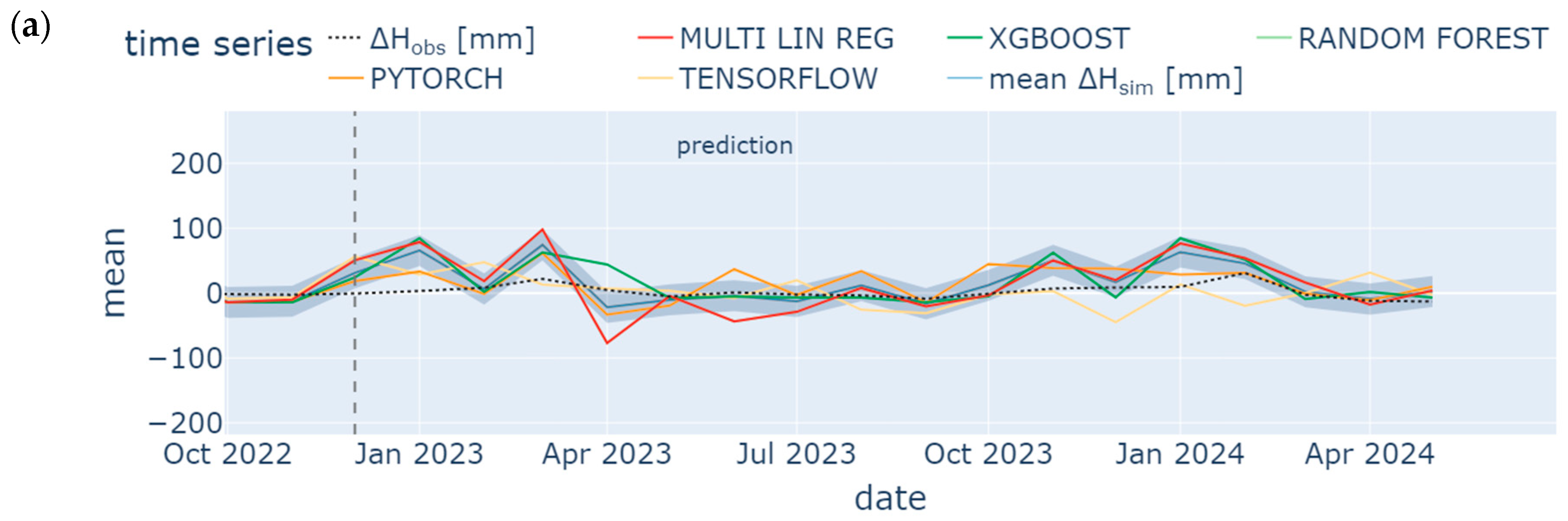
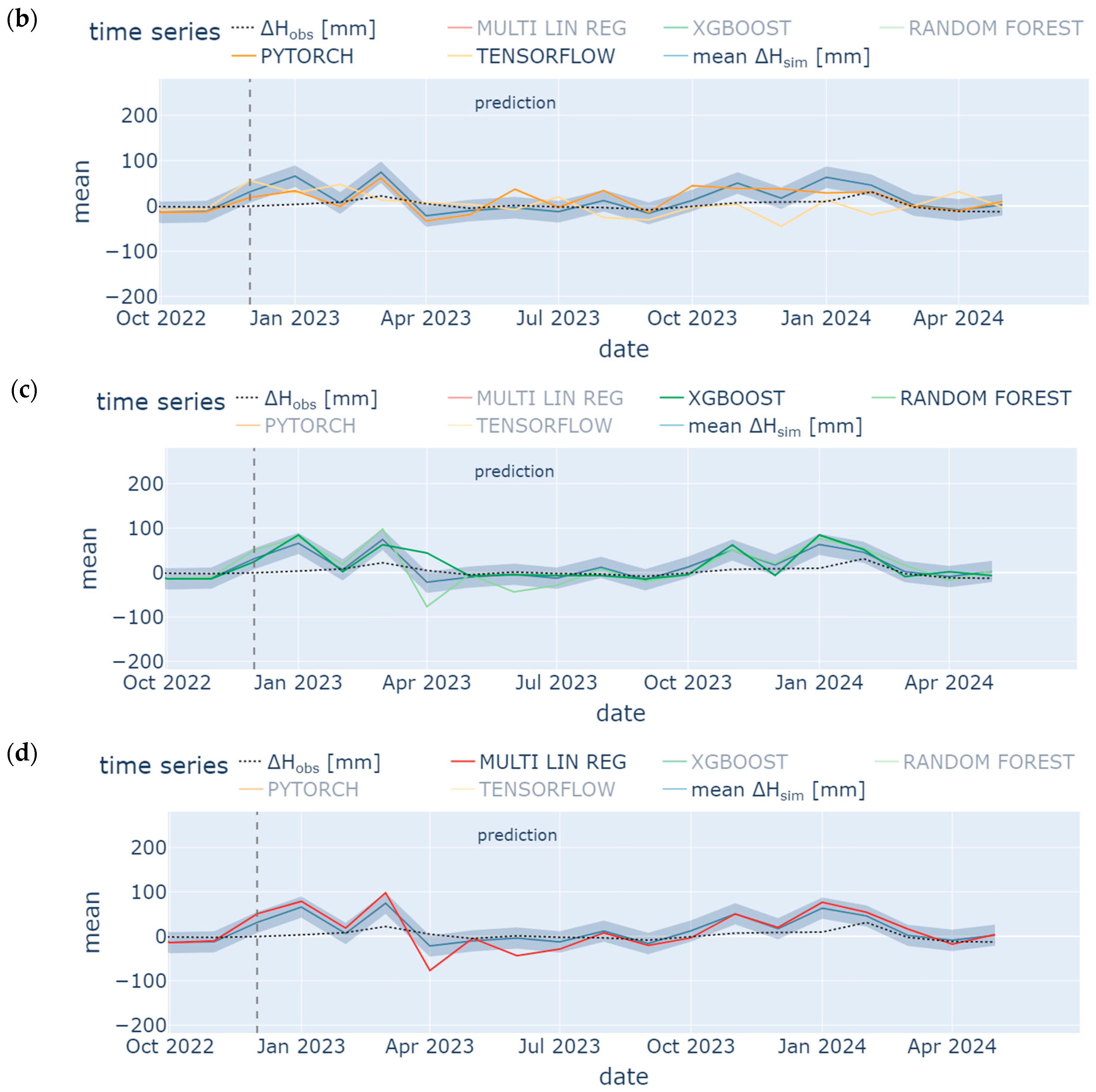
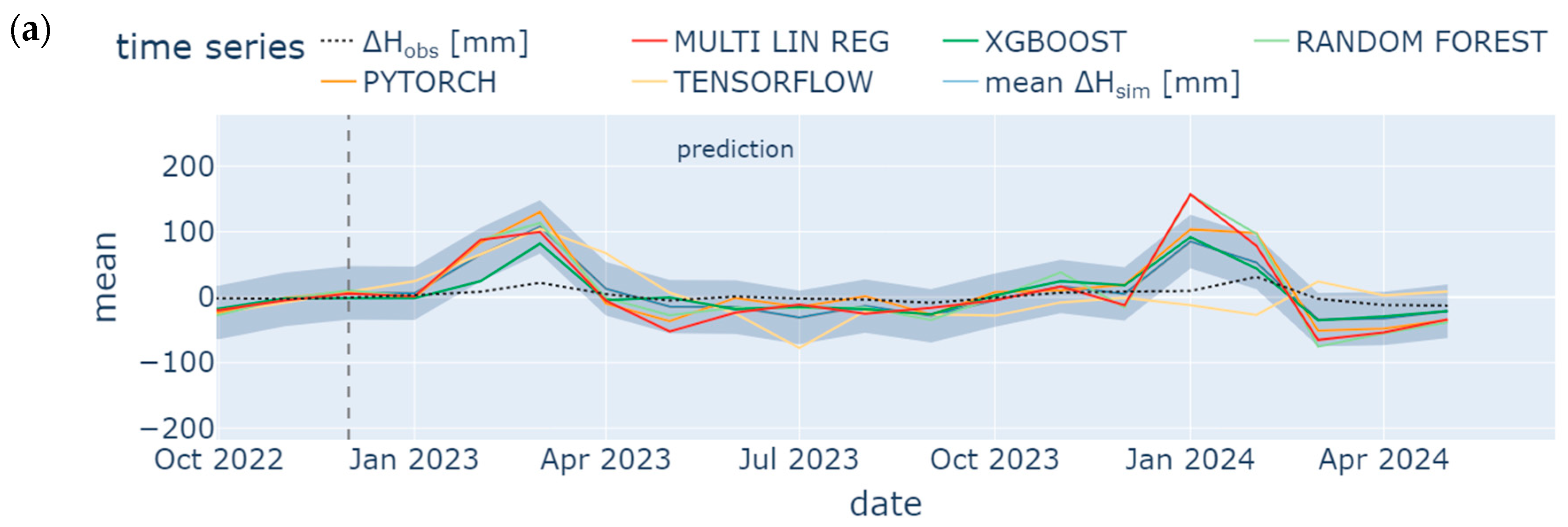
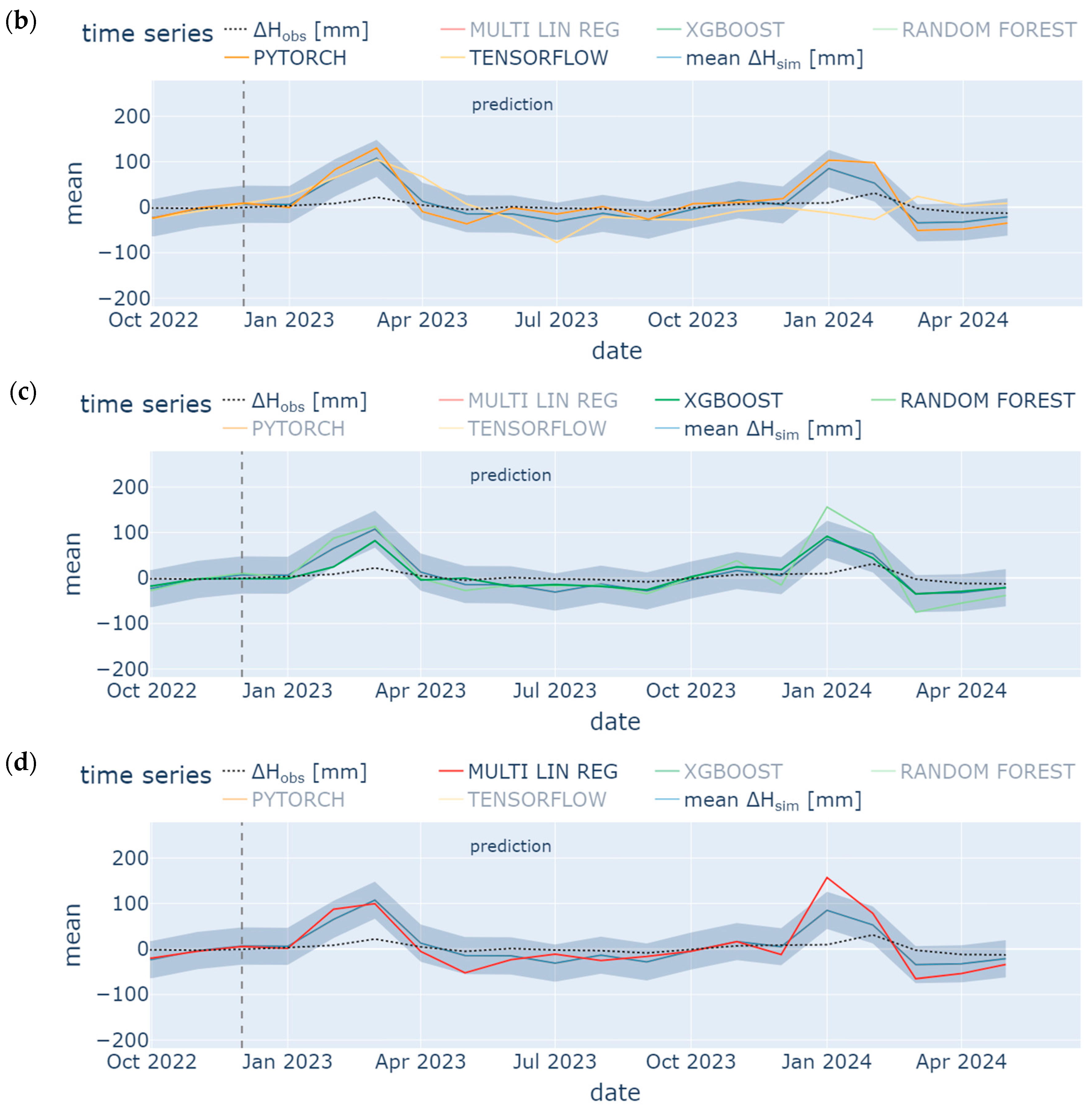
4.3. Prediction

Figure 13 and Figure 14 show all the predicted $\Delta H_{sim}^{BART}$ time series covering the period January 2023 to May 2024, similarly visualized in previous figures. In agreement with previously trained and reconstructed time series, the predicted values behave analogously and show less variability during the hydrological summer months from May 2023 to November 2023. Higher $\Delta H_{sim}^{BART}$ variability occurs during the hydrological winter months, in particular April 2023 (mean −27 mm) and November 2023 (mean 47 mm) for models based on input data from BEEN and March 2023 (mean 106 mm) and January 2024 (mean 91 mm) for models based on input data from SWG.

5. Discussion

5.1. Significance of Simplified Machine Learning Models and Input Data

Due to scarce and interrupted groundwater monitoring data, it can become difficult to calibrate numerical flow and transport models for scenario prognosis. Therefore, the present study deals with the reconstruction and prediction of missing data in groundwater time series using Deep Learning (TensorFlow, PyTorch) and classical machine learning (ML) methods (Random Forest, XGBoost, Multiple Linear Regression). The results show that these ML methods can be a tool to fill data gaps by learning from the input data. However, ML methods struggle to predict extreme values as shown in the present study. Therefore, when physical measurements are available or feasible to execute, those should be favored over such artificial data for extreme events. The underestimation of extreme values limits the present models, especially when future scenarios are calculated. These future climate scenarios predict a larger abundance of extreme values (in form of, e.g., large precipitation with short duration) [84]. An adequate use of ML methods for predicting extreme values based on climate scenarios should therefore be connected to a new train/test procedure incorporating training and test data containing such extreme values.

The present study shows that ML methods are a valid alternative to, e.g., complex and time-consuming numerical groundwater flow models. A well-trained ML model with a good correlation between input data and output data may lead to similar results compared with a calibrated and validated numerical groundwater flow model. ML models also enable real-time modeling, while the runtime of numerical groundwater flow models at the catchment scale can be in the range of hours. However, ML models are limited to their specific output (in our case, the groundwater level at a certain location), while numerical models provide multidimensional potential fields that enable flexible in-depth post-processing of data in form of, e.g., flow paths, travel times, flow regimes in specific aquifers, and more. Subsequently, for specific applications such as groundwater management, adequate ML models are valuable, effective, and precise tools.

When developing ML models, high model complexity leads to a larger search space for hyperparameters, which can significantly increase the computational resources required for hyperparameter optimization. According to Hancock and Khoshgoftaar [85], this is particularly evident for large datasets where the cost of tuning can be substantial. Therefore, the present study uses different ML methods with few but relevant hyperparameters (e.g., learning rate, n estimators) and input data (e.g., precipitation, groundwater head differences). According to A Ilemobayo, Durodola [86], adequate hyperparameters can significantly impact a model’s performance. This results in reduced computational model complexity needing fewer but robust hyperparameters, short computation times, and a decreased risk of overfitting.

A careful selection of input data is essential when using ML methods in groundwater related applications. Therefore, analyzing the data for dependencies or correlations prior to model development is crucial. According to Maliva [87], precipitation has the highest influence on shallow groundwater recharge [81,88,89,90]; hence, precipitation is selected as input data in the present study. If precipitation is not sufficient for ML model development, input data representing other physical processes and elements of the water balance affecting groundwater have to be included. For example, if evaporation is found to have a significant impact on groundwater, Wunsch, Liesch [36] show that temperature data can be used as a valid proxy. Clearly, the accuracy of the model depends on the accuracy of the input data, which propagates through the steps of model building, being inflated by model inaccuracies, and leading to an often uncertain error in the model result. While measurement errors in groundwater potentials [91,92] and precipitation [93,94] can be quantified, the overall error from the model can only be quantified indirectly by comparison with physical measurements, if measurements are available. In the present study, when reconstructing unknown time series, no physical measurements are available and the model accuracy is unknown. Therefore, prior to performing such a reconstruction, it is necessary to establish a level of confidence in the model results by validating the model in an adequate way. Furthermore, monthly ΔH have been impacted by evapotranspiration, land use, media properties, diffuse sources, and sinks, among others [95,96] and serve therefore as an additional input in the present study.

5.2. Uncertainty Reduction in Gap-Based Time Series

The present study uses ML methods as a preprocessing step for numerical models in order to reduce uncertainties and incompleteness in calibration data. Therefore, missing monthly $\Delta H_{obs}^{BART}$ values within a time series for Bartensleben based on Beendorf or Schwanefeld-Güte are reconstructed and predicted. In order to gain an overall understanding of the hydrological trend within the time series, the simulated time series from different ML models are compared and then averaged. This model ensemble approach reduces the uncertainty of each individual model. This model ensemble can be compared to climate scenario simulations [97]. By creating an ensemble of the ML model results around the observed groundwater head time series, the errors of the individual models are averaged such that the overall error margin decreases [98].

In accordance with Tsuchihara, Yoshimoto [99], the variabilities shown by the completed time series indicate seasonal fluctuations due to the periodic return of groundwater discharge and recharge. Typically, low values occur during hydrological summer months and higher fluctuations during hydrological winter months, which is in line with Chen, Wen [96]. Furthermore, supporting the present results, Huang, Krysanova [15] stated that during summer months, smaller runoffs occur due to increased evapotranspiration [100] and warmer temperatures, while in winter higher runoffs occur due to low evapotranspiration. This indicates that precipitation directly influences groundwater dynamics as a proxy for groundwater recharge, which is also shown in Chen, Grasby [101] and Heo, Kim [102]. Especially, groundwater head differences in summer showing notably decreasing trends, with a mean simulated decrease $\Delta H_{sim,SWG}^{BART}$ of −17 mm (compared with the observed decrease $\Delta H_{obs}^{BART}$ −27 mm) for the past 34 years, indicating declining groundwater levels and therefore less groundwater storage and recharge. This is in line with Neukum and Azzam [103] and Wunsch, Liesch [43], where the latter investigated the influence of low groundwater periods using machine learning and identified summer as the most important season for low groundwater levels.

Clearly, ML models can only represent such trends if they are included in the input and training data. If trends change in the future, the present models need new input data in order to predict consistent results. As previously described, the ML models also need to be retrained due to unseen extreme events. Therefore, continuous measurements followed by trend analyses are required to ensure the validity of the present model for predictions into the far future. However, for the time given, the present study reveals that the applied ML methods show reasonable results with respect to seasonal climate variations and local conditions in Bartensleben, such that a combination of few input data and less complex trained and tested ML methods are suitable for reconstruction and short-term prediction of missing data in groundwater head time series.

5.3. Drawbacks and Limitations of the Present Study

The present study shows that ML models can accurately calculate groundwater time series at a specific location in the Allertal. However, a drawback of the study is that the ML models are only applicable to a specific location. Even if all considered conditions are similar, the present ML models can only be applied to other locations if the input data correlate with the output data in a similar way. If a ML model from the present study is used at a different location without carrying out an explanatory data analysis, unknown inputs such as, e.g., groundwater pumping can lead to a significant model error. Therefore, it is crucial to perform a detailed explanatory data analysis prior to model training.

Another drawback of the present study is that the training data do not allow accurately predicting extreme values. This is simply because the training data do not contain such values. For more accurate and robust predictions of extreme values, the present model should be retrained with more data, including extremes. However, at present time, available data are limited to the time series used in the present study.

A further drawback could be related to the selection of the hyperparameters and their bandwidths. Although multiple hyperparameter combinations were tested, it is possible that a hyperparameter combination with values beyond the selected bandwidth and/or an additional hyperparameter not selected in this study could result in better model performance. However, the training of five different ML methods, each with larger bandwidths of multiple hyperparameters, is time-consuming. Therefore, in the present study, a focus on the most affecting hyperparameter in each of the five ML models was performed in order to prioritize and save time.

6. Summary and Conclusions

The main aim of the present study is to establish a consistent groundwater head time series for future use in numerical modeling of flow and transport processes in the Allertal, Saxony-Anhalt, Germany. Therefore, current groundwater data gaps within the Bartensleben monitoring time series were filled by using a model ensemble of five machine learning (ML) approaches, consisting of TensorFlow, PyTorch (Deep Learning), Random Forest, XGBoost, and Multiple Linear Regression. A correlation analysis showed that the precipitation and difference in groundwater head data are sufficient for an adequate model building. Therefore, these few input data from one of the two neighboring and consistent state-monitoring stations (Beendorf (BEEN) or Schwanefeld-Güte (SWG)) were used to train the multiple ML models to reconstruct and to predict the monthly groundwater head time series at Bartensleben. To achieve these aims a total four steps were necessary. Step 1 and 2 consisted of ML model training and testing. Finally, the models were applied to (Step 3) reconstruct and (Step 4) predict missing groundwater heads based on data from the two neighboring stations BEEN or SWG.

In summary, key contributions of the present study are as follows:

(1)

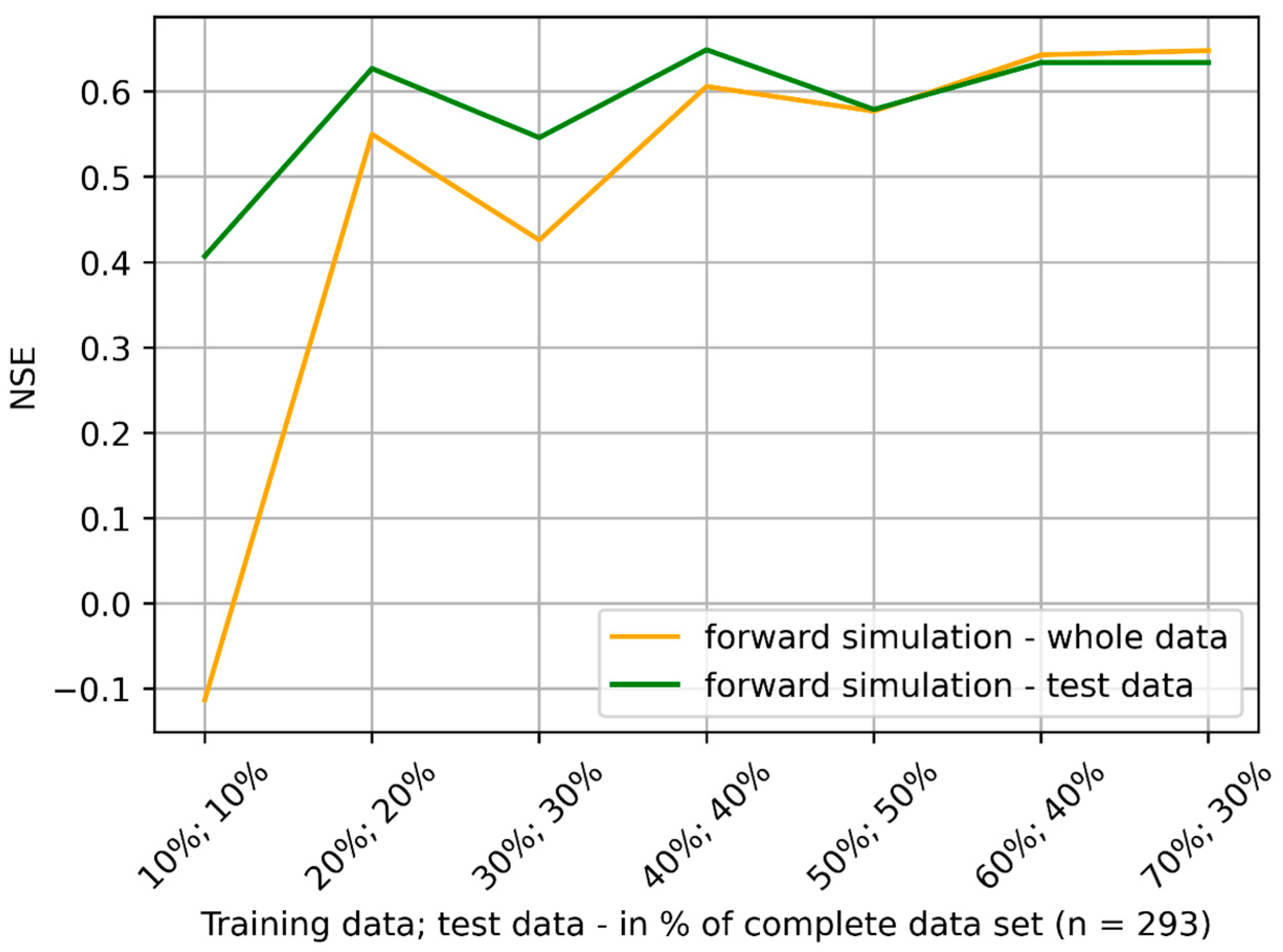
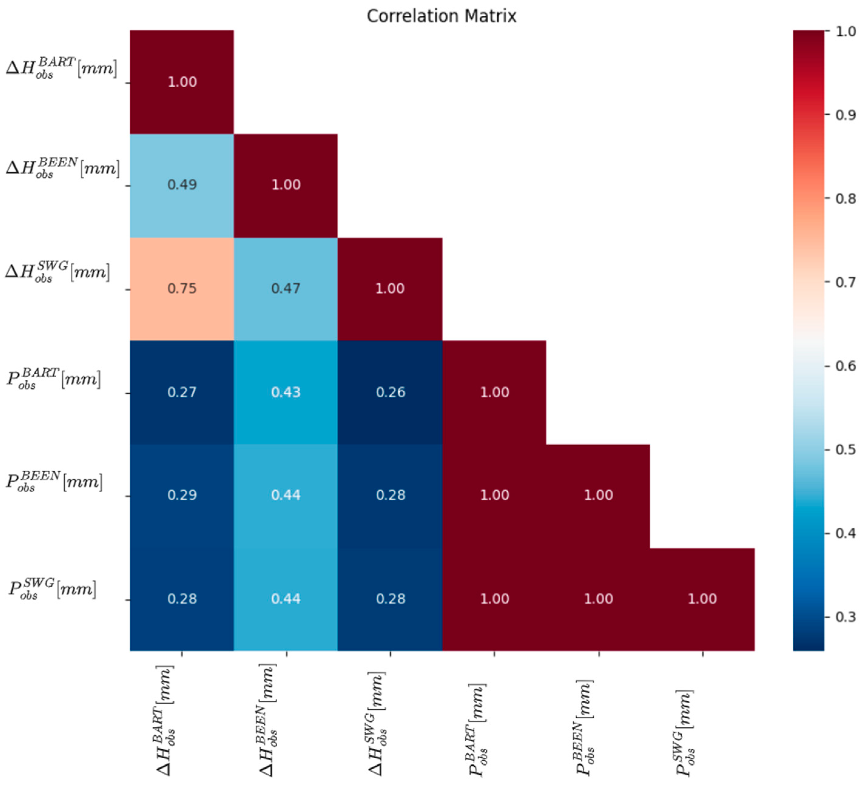
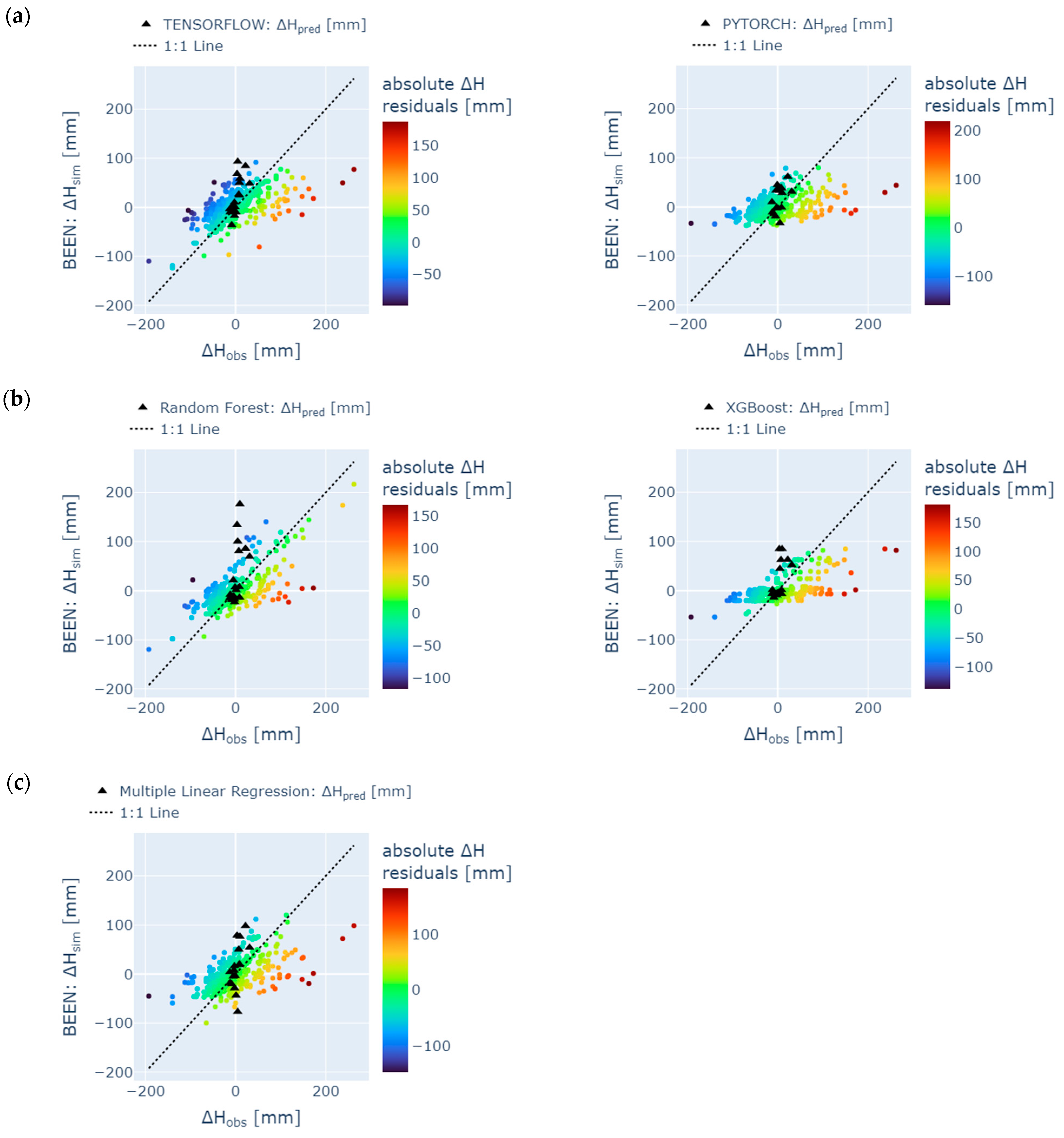
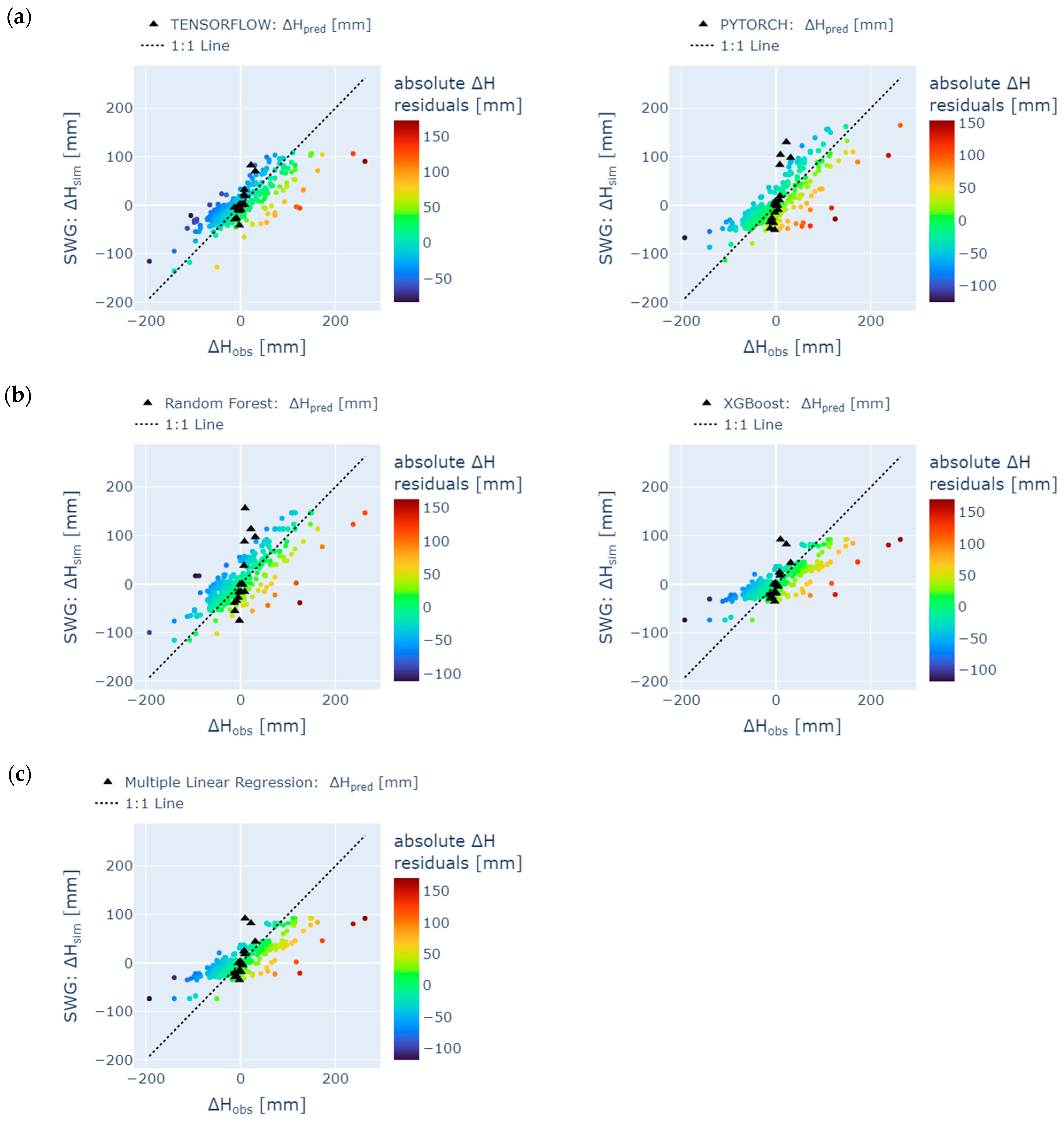
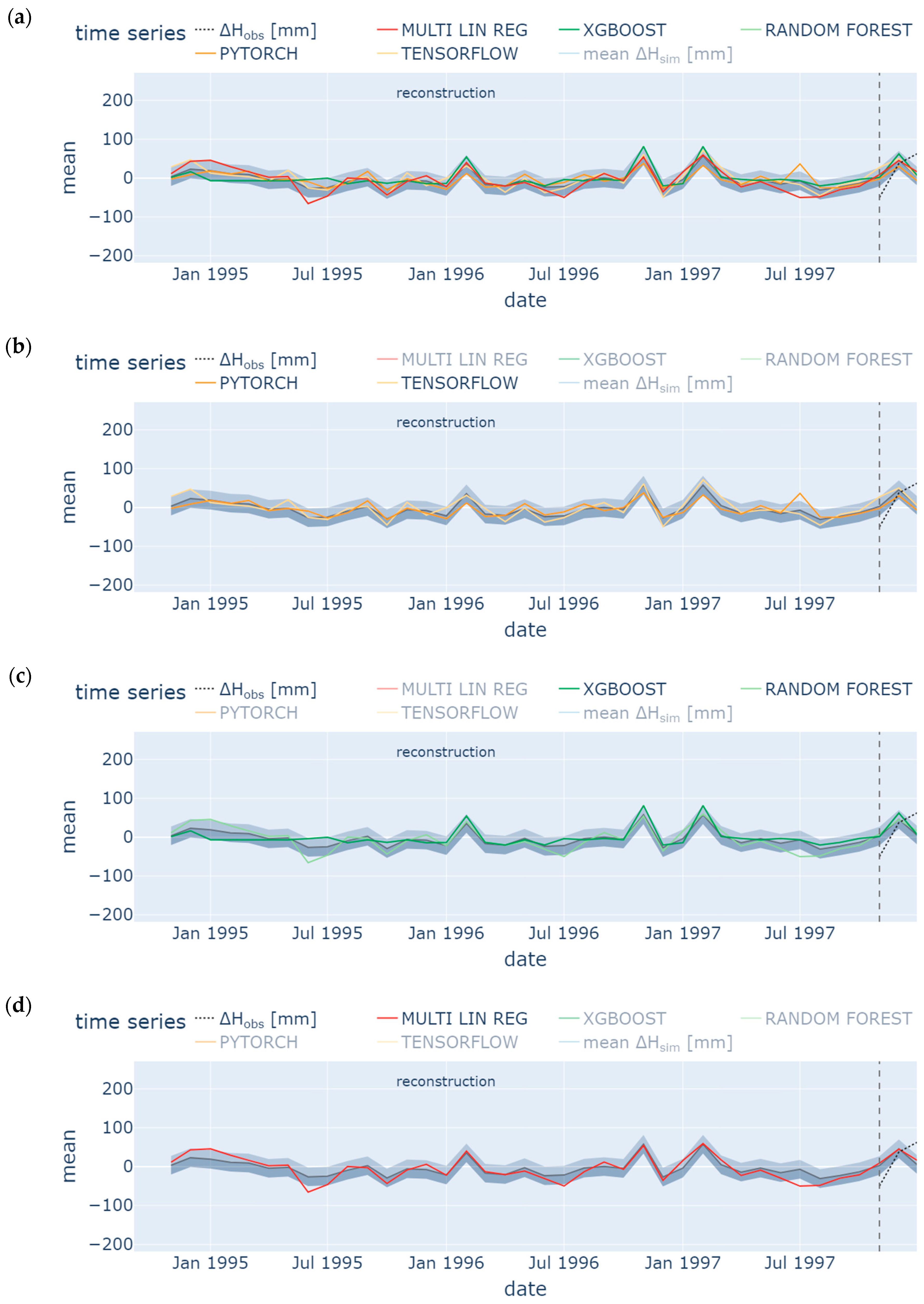
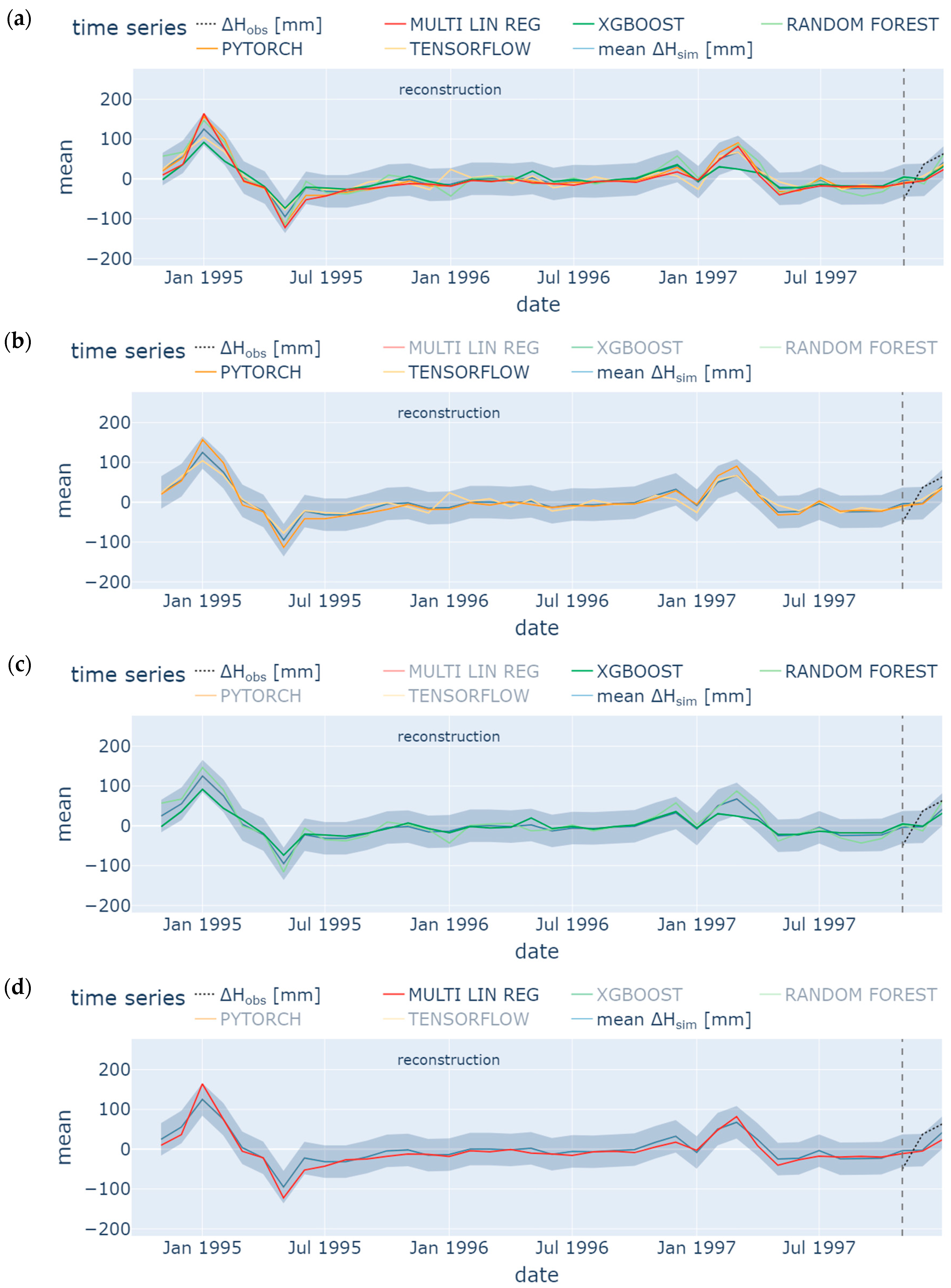
Missing groundwater heads were successfully reconstructed (1995 to 1997) and predicted (January 2023 to May 2024) by using few input data. However, only the model ensemble based on data from the neighboring station SWG gave adequate results. It was shown in the prior-to-model-development explorative data analysis that data from SWG and BART correlate (groundwater head differences from both stations show NSE = 0.75), which leads to an accurate model in the present study (NSE = 0.65 (test) to 0.71 (training) for one exemplary ML model). In contrast, BART and BEEN show a low grade of data correlation (for groundwater head differences NSE = 0.49). The model ensemble predicts groundwater head differences with an insufficient accuracy (NSE = 0.3 (test) to 0.46 (training) for an exemplary ML model). Hence, if data are sufficiently correlated, ML methods are applicable also for a time series data consisting of few data. The considered monitoring stations have to be located in the same study area. Overfitting can be challenging such that a suitable model should have similar training and prediction NSEs to avoid this behavior.

(2)

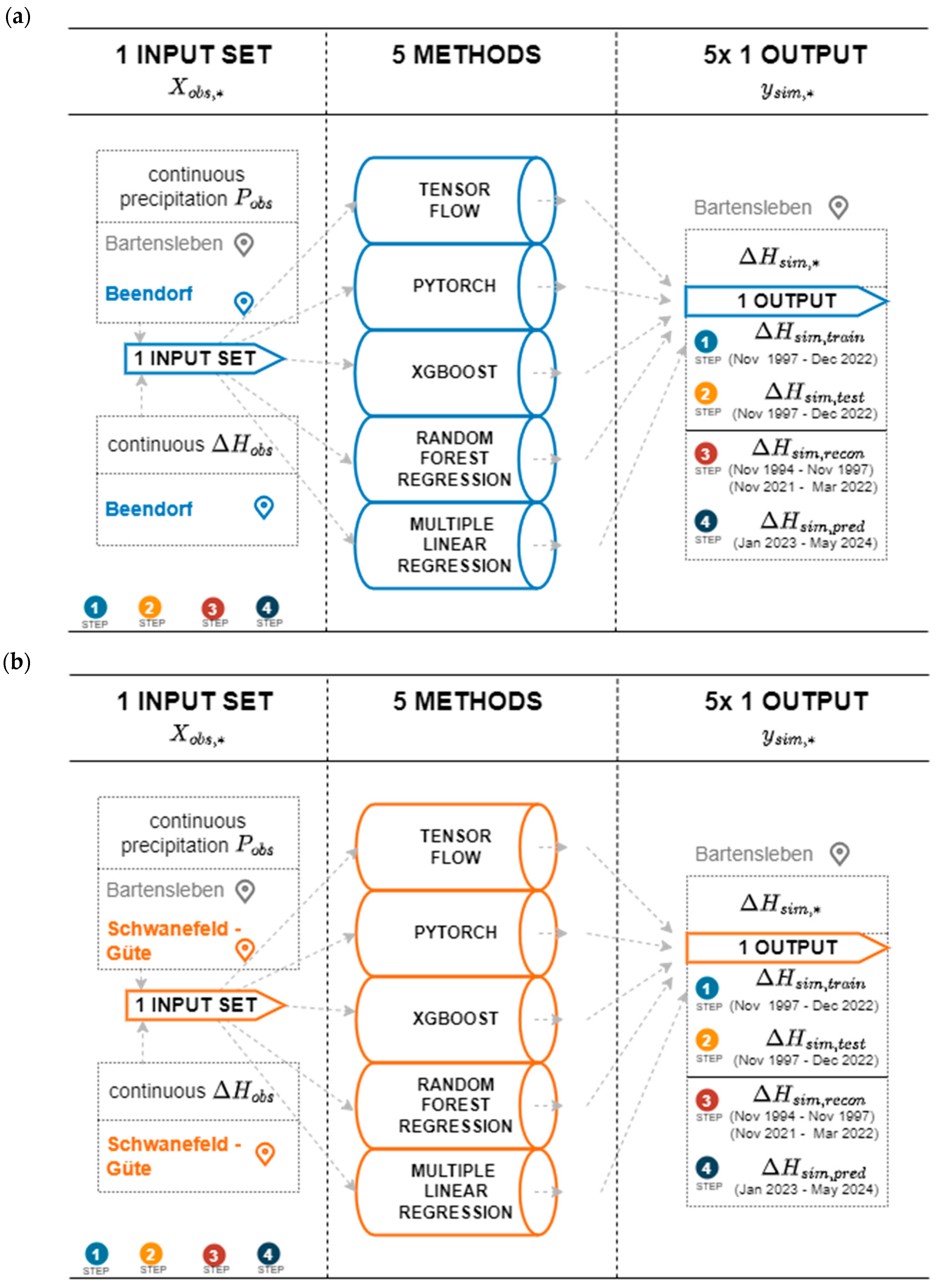
TensorFlow, PyTorch, Random Forest, XGBoost, and Multiple Linear Regression show similar results, especially during hydrological summer months when low variation occurred; hence, for time series analysis, each ML methods is applicable in order to detect seasonal trend analysis. Specifically, the Random Forest model and the ANN using the TensorFlow package performed best with a train/test NSE of 0.7/0.53 and 0.71/0.65, respectively. However, results from the latter were less prone to overfitting. These results confirm some findings from the literature [104]. However, other studies have shown that the support vector machine method (which was not considered in the present study) outperformed the ANN [105], while XGBoost outperformed the ANN [70]. The most appropriate ML method may vary from location to location. It depends on various factors such as the specific characteristics of the dataset, the location with its specific conditions, and the experience of the operator training, testing, and analyzing the model.

The present study reveals that ML models can be trained with few input data. The model ensemble developed in the present study provides further insights into the hydrogeological dynamic conditions of the Allertal and enables further future prediction. The present study may contribute to the generation of the consistent groundwater head time series for the calibration process of a numerical flow model. Such consistent time series can increase the acceptance and confidence in the numerical modeling results. While this study is more of a case study, to our knowledge there is no fundamental investigation yet of the required length of correlated groundwater head time series for the development of ML models in the literature. This should be a subject of future research.

References

- Hayley, K. The present state and future application of cloud computing for numerical groundwater modeling. Groundwater 2017, 55, 678–682. [Google Scholar] [CrossRef]
- Zhou, Y.; Li, W. A review of regional groundwater flow modeling. Geosci. Front. 2011, 2, 205–214. [Google Scholar] [CrossRef]
- Hill, M.C.; Tiedeman, C.R. Effective Groundwater Model Calibration: With Analysis of Data, Sensitivities, Predictions, and Uncertainty; John Wiley & Sons: Hoboken, NJ, USA, 2007. [Google Scholar]
- Adams, K.H.; Reager, J.T.; Rosen, P.; Wiese, D.N.; Farr, T.G.; Rao, S.; Haines, B.J.; Argus, D.F.; Liu, Z.; Smith, R.; et al. Remote sensing of groundwater: Current capabilities and future directions. Water Resour. Res. 2022, 58, e2022WR032219. [Google Scholar] [CrossRef]
- Brunner, P.; Hendricks Franssen, H.-J.; Kgotlhang, L.; Bauer-Gottwein, P.; Kinzelbach, W. How can remote sensing contribute in groundwater modeling? Hydrogeol. J. 2007, 15, 5–18. [Google Scholar] [CrossRef]
- Cardenas, M.B.; Zamora, P.B.; Siringan, F.P.; Lapus, M.R.; Rodolfo, R.S.; Jacinto, G.S.; San Diego-McGlone, M.L.; Villanoy, C.L.; Cabrera, O.; Senal, M.I. Linking regional sources and pathways for submarine groundwater discharge at a reef by electrical resistivity tomography, 222Rn, and salinity measurements. Geophys. Res. Lett. 2010, 37. [Google Scholar] [CrossRef]
- Tran, T.V.; Buckel, J.; Maurischat, P.; Tang, H.; Yu, Z.; Hördt, A.; Guggenberger, G.; Zhang, F.; Schwalb, A.; Graf, T. Delineation of a Quaternary aquifer using integrated hydrogeological and geophysical estimation of hydraulic conductivity on the Tibetan Plateau, China. Water 2021, 13, 1412. [Google Scholar] [CrossRef]
- Barchard, K.A.; Pace, L.A. Preventing human error: The impact of data entry methods on data accuracy and statistical results. Comput. Hum. Behav. 2011, 27, 1834–1839. [Google Scholar] [CrossRef]
- Osborne, J.W. Dealing with Missing or Incomplete Data: Debunking the Myth of Emptiness. In Best Practices in Data Cleaning: A Complete Guide to Everything You Need to Do Before and After Collecting Your Data; SAGE Publications, Inc.: Newbury Park, CA, USA, 2013; pp. 105–138. [Google Scholar]
- Kang, H. The prevention and handling of the missing data. Korean J. Anesthesiol. 2013, 64, 402–406. [Google Scholar] [CrossRef] [PubMed]
- Hunt, R.J.; Fienen, M.N.; White, J.T. Revisiting “an exercise in groundwater model calibration and prediction” after 30 years: Insights and new directions. Groundwater 2020, 58, 168–182. [Google Scholar] [CrossRef]
- Freyberg, D.L. An exercise in ground-water model calibration and prediction. Groundwater 1988, 26, 350–360. [Google Scholar] [CrossRef]
- Hodgson, F.D. The use of multiple linear regression in simulating ground-water level responses. Groundwater 1978, 16, 249–253. [Google Scholar] [CrossRef]
- Jobson, J.D. Multiple Linear Regression, in Applied Multivariate Data Analysis: Regression and Experimental Design; Springer: New York, NY, USA, 1991; pp. 219–398. [Google Scholar]
- Huang, S.; Krysanova, V.; Österle, H.; Hattermann, F.F. Simulation of spatiotemporal dynamics of water fluxes in Germany under climate change. Hydrol. Process. 2010, 24, 3289–3306. [Google Scholar] [CrossRef]
- Sahoo, S.; Jha, M.K. Groundwater-level prediction using multiple linear regression and artificial neural network techniques: A comparative assessment. Hydrogeol. J. 2013, 21, 1865–1887. [Google Scholar] [CrossRef]
- Krizhevsky, A.; Sutskever, I.; Hinton, G.E. ImageNet classification with deep convolutional neural networks. Commun. ACM 2017, 60, 84–90. [Google Scholar] [CrossRef]
- Koch, J.; Berger, H.; Henriksen, H.J.; Sonnenborg, T.O. Modelling of the shallow water table at high spatial resolution using random forests. Hydrol. Earth Syst. Sci. 2019, 23, 4603–4619. [Google Scholar] [CrossRef]
- Fathian, F. Introduction of multiple/multivariate linear and nonlinear time series models in forecasting streamflow process. In Advances in Streamflow Forecasting; Elsevier: Amsterdam, The Netherlands, 2021; pp. 87–113. [Google Scholar]
- Wunsch, A.; Liesch, T.; Broda, S. Groundwater level forecasting with artificial neural networks: A comparison of long short-term memory (LSTM), convolutional neural networks (CNNs), and non-linear autoregressive networks with exogenous input (NARX). Hydrol. Earth Syst. Sci. 2021, 25, 1671–1687. [Google Scholar] [CrossRef]
- Dastjerdi, S.Z.; Sharifi, E.; Rahbar, R.; Saghafian, B. Downscaling WGHM-Based Groundwater Storage Using Random Forest Method: A Regional Study over Qazvin Plain, Iran. Hydrology 2022, 9, 179. [Google Scholar] [CrossRef]
- Kratzert, F.; Gauch, M.; Nearing, G.; Klotz, D. NeuralHydrology—A Python library for Deep Learning research in hydrology. J. Open Source Softw. 2022, 7, 4050. [Google Scholar] [CrossRef]
- Ehteram, M.; Banadkooki, F.B. A Developed Multiple Linear Regression (MLR) Model for Monthly Groundwater Level Prediction. Water 2023, 15, 3940. [Google Scholar] [CrossRef]
- Kumar, V.; Kedam, N.; Sharma, K.V.; Mehta, D.J.; Caloiero, T. Advanced Machine Learning Techniques to Improve Hydrological Prediction: A Comparative Analysis of Streamflow Prediction Models. Water 2023, 15, 2572. [Google Scholar] [CrossRef]
- Latif, S.D.; Ahmed, A.N. A review of deep learning and machine learning techniques for hydrological inflow forecasting. Environ. Dev. Sustain. 2023, 25, 12189–12216. [Google Scholar] [CrossRef]
- Seidu, J.; Ewusi, A.; Kuma, J.S.Y.; Ziggah, Y.Y.; Voigt, H.-J. Impact of data partitioning in groundwater level prediction using artificial neural network for multiple wells. Int. J. River Basin Manag. 2023, 21, 639–650. [Google Scholar] [CrossRef]
- Logashenko, D.; Litvinenko, A.; Tempone, R.; Wittum, G. Estimation of uncertainties in the density driven flow in fractured porous media using MLMC. arXiv 2024, arXiv:2404.18003. [Google Scholar] [CrossRef]
- Bakker, M.; Schaars, F. Solving groundwater flow problems with time series analysis: You may not even need another model. Groundwater 2019, 57, 826–833. [Google Scholar] [CrossRef] [PubMed]
- LHW. Geodatenportal. 07.11.2024 07.01.2024. Available online: https://gld.lhw-sachsen-anhalt.de/ (accessed on 25 June 2024).
- Kluyver, T.; Ragan-Kelley, B.; Pérez, F.; Granger, B.; Bussonnier, M.; Frederic, J.; Kelley, K.; Hamrick, J.; Grout, J.; Corlay, S. Jupyter Notebooks–a publishing format for reproducible computational workflows. In Positioning and Power in Academic Publishing: Players, Agents and Agendas; IOS Press: Amsterdam, The Netherlands, 2016; pp. 87–90. [Google Scholar]
- Li, B.; Yang, G.; Wan, R.; Dai, X.; Zhang, Y. Comparison of random forests and other statistical methods for the prediction of lake water level: A case study of the Poyang Lake in China. Hydrol. Res. 2016, 47, 69–83. [Google Scholar] [CrossRef]
- DWD. Climate Data Center. 07.11.2024 05.01.2024. Available online: https://www.dwd.de/DE/leistungen/cdc/climate-data-center.html?nn=17626 (accessed on 29 June 2024).
- QGIS. QGIS Geographic Information System. 2024. Available online: http://www.qgis.org (accessed on 25 May 2024).
- Sherman, G. The PyQGIS Programmer’s Guide; Locate Press: London, UK, 2014. [Google Scholar]
- Pang, J.; Zhang, H.; Xu, Q.; Wang, Y.; Wang, Y.; Zhang, O.; Hao, J. Hydrological evaluation of open-access precipitation data using SWAT at multiple temporal and spatial scales. Hydrol. Earth Syst. Sci. 2020, 24, 3603–3626. [Google Scholar] [CrossRef]
- Wunsch, A.; Liesch, T.; Broda, S. Deep learning shows declining groundwater levels in Germany until 2100 due to climate change. Nat. Commun. 2022, 13, 1221. [Google Scholar] [CrossRef] [PubMed]
- Sahour, H.; Gholami, V.; Vazifedan, M. A comparative analysis of statistical and machine learning techniques for mapping the spatial distribution of groundwater salinity in a coastal aquifer. J. Hydrol. 2020, 591, 125321. [Google Scholar] [CrossRef]
- TensorFlow Developers. TensorFlow, v2.12.0; Zenodo: Geneva, Switzerland, 2024. [Google Scholar]
- Paszke, A.; Gross, S.; Massa, F.; Lerer, A.; Bradbury, J.; Chanan, G.; Killeen, T.; Lin, Z.; Gimelshein, N.; Antiga, L. PyTorch; v.2.3.1. An Imperative Style, High-Performance Deep Learning Library. Advances in Neural Information Processing Systems 32; Zenodo: Geneva, Switzerland, 2019. [Google Scholar]
- Joy, T.T.; Rana, S.; Gupta, S.; Venkatesh, S. Hyperparameter tuning for big data using Bayesian optimisation. In Proceedings of the 2016 23rd International Conference on Pattern Recognition (ICPR), Cancun, Mexico, 4–8 December 2016. [Google Scholar]
- Kim, J.-Y.; Cho, S.-B. Evolutionary optimization of hyperparameters in deep learning models. In Proceedings of the 2019 IEEE Congress on Evolutionary Computation (CEC), Wellington, New Zealand, 10–13 June 2019. [Google Scholar]
- Nematzadeh, S.; Kiani, F.; Torkamanian-Afshar, M.; Aydin, N. Tuning hyperparameters of machine learning algorithms and deep neural networks using metaheuristics: A bioinformatics study on biomedical and biological cases. Comput. Biol. Chem. 2022, 97, 107619. [Google Scholar] [CrossRef] [PubMed]
- Wunsch, A.; Liesch, T.; Goldscheider, N. Towards understanding the influence of seasons on low-groundwater periods based on explainable machine learning. Hydrol. Earth Syst. Sci. 2024, 28, 2167–2178. [Google Scholar] [CrossRef]
- Abadi, M.; Barham, P.; Chen, J.; Chen, Z.; Davis, A.; Dean, J.; Devin, M.; Ghemawat, S.; Irving, G.; Isard, M. TensorFlow: A System for Large-Scale Machine Learning. In Proceedings of the 12th USENIX symposium on operating systems design and implementation (OSDI 16), Savannah, GA, USA, 2–4 November 2016. [Google Scholar]
- Qin, J.; Liang, J.; Chen, T.; Lei, X.; Kang, A. Simulating and Predicting of Hydrological Time Series Based on TensorFlow Deep Learning. Pol. J. Environ. Stud. 2019, 28, 795–802. [Google Scholar] [CrossRef]
- Chollet, F. Deep Learning with Python; Simon and Schuster: New York, NY, USA, 2021. [Google Scholar]
- Bowes, B.D.; Sadler, J.M.; Morsy, M.M.; Behl, M.; Goodall, J.L. Forecasting groundwater table in a flood prone coastal city with long short-term memory and recurrent neural networks. Water 2019, 11, 1098. [Google Scholar] [CrossRef]
- Solgi, R.; Loaiciga, H.A.; Kram, M. Long short-term memory neural network (LSTM-NN) for aquifer level time series forecasting using in-situ piezometric observations. J. Hydrol. 2021, 601, 126800. [Google Scholar] [CrossRef]
- Bebis, G.; Georgiopoulos, M. Feed-forward neural networks. IEEE Potentials 1994, 13, 27–31. [Google Scholar] [CrossRef]
- Berkhahn, S.; Fuchs, L.; Neuweiler, I. An ensemble neural network model for real-time prediction of urban floods. J. Hydrol. 2019, 575, 743–754. [Google Scholar] [CrossRef]
- McCulloch, W.S.; Pitts, W. A logical calculus of the ideas immanent in nervous activity. Bull. Math. Biophys. 1943, 5, 115–133. [Google Scholar] [CrossRef]
- Harris, C.R.; Millman, K.J.; Van Der Walt, S.J.; Gommers, R.; Virtanen, P.; Cournapeau, D.; Wieser, E.; Taylor, J.; Berg, S.; Smith, N.J. Array programming with NumPy. Nature 2020, 585, 357–362. [Google Scholar] [CrossRef] [PubMed]
- Abbas, A.; Boithias, L.; Pachepsky, Y.; Kim, K.; Chun, J.A.; Cho, K.H. AI4Water v1.0, an open-source python package for modeling hydrological time series using data-driven methods. Geosci. Model Dev. 2022, 15, 3021–3039. [Google Scholar] [CrossRef]
- Novac, O.-C.; Chirodea, M.C.; Novac, C.M.; Bizon, N.; Oproescu, M.; Stan, O.P.; Gordan, C.E. Analysis of the Application Efficiency of TensorFlow and PyTorch in Convolutional Neural Network. Sensors 2022, 22, 8872. [Google Scholar] [CrossRef] [PubMed]
- Jiang, P.; Shuai, P.; Sun, A.; Mudunuru, M.K.; Chen, X. Knowledge-informed deep learning for hydrological model calibration: An application to Coal Creek Watershed in Colorado. Hydrol. Earth Syst. Sci. 2023, 27, 2621–2644. [Google Scholar] [CrossRef]
- Shin, M.-J.; Kim, J.-W.; Moon, D.-C.; Lee, J.-H.; Kang, K.G. Comparative analysis of activation functions of artificial neural network for prediction of optimal groundwater level in the middle mountainous area of Pyoseon watershed in Jeju Island. J. Korea Water Resour. Assoc. 2021, 54, 1143–1154. [Google Scholar]
- Rodriguez-Galiano, V.; Mendes, M.P.; Garcia-Soldado, M.J.; Chica-Olmo, M.; Ribeiro, L. Predictive modeling of groundwater nitrate pollution using Random Forest and multisource variables related to intrinsic and specific vulnerability: A case study in an agricultural setting (Southern Spain). Sci. Total Environ. 2014, 476, 189–206. [Google Scholar] [CrossRef]
- Genuer, R.; Poggi, J.M. Random Forests with R; Springer: Berlin/Heidelberg, Germany, 2020. [Google Scholar]
- Louppe, G. Understanding random forests: From theory to practice. arXiv 2014, arXiv:1407.7502. [Google Scholar]
- Fratello, M.; Tagliaferri, R. Decision trees and random forests. In Encyclopedia of Bioinformatics and Computational Biology: ABC of Bioinformatics; Elsvier: Amsterdam, The Netherlands, 2018; Volume 1. [Google Scholar]
- Amro, A.; Al-Akhras, M.; Hindi, K.E.; Habib, M.; Shawar, B.A. Instance Reduction for Avoiding Overfitting in Decision Trees. J. Intell. Syst. 2021, 30, 438–459. [Google Scholar] [CrossRef]
- Naghibi, S.A.; Ahmadi, K.; Daneshi, A. Application of support vector machine, random forest, and genetic algorithm optimized random forest models in groundwater potential mapping. Water Resour. Manag. 2017, 31, 2761–2775. [Google Scholar] [CrossRef]
- Tyralis, H.; Papacharalampous, G.; Langousis, A. A brief review of random forests for water scientists and practitioners and their recent history in water resources. Water 2019, 11, 910. [Google Scholar] [CrossRef]
- Pham, L.T.; Luo, L.; Finley, A. Evaluation of random forests for short-term daily streamflow forecasting in rainfall-and snowmelt-driven watersheds. Hydrol. Earth Syst. Sci. 2021, 25, 2997–3015. [Google Scholar] [CrossRef]
- Madani, A.; Niyazi, B. Groundwater Potential Mapping Using Remote Sensing and Random Forest Machine Learning Model: A Case Study from Lower Part of Wadi Yalamlam, Western Saudi Arabia. Sustainability 2023, 15, 2772. [Google Scholar] [CrossRef]
- Moghaddam, D.D.; Rahmati, O.; Panahi, M.; Tiefenbacher, J.; Darabi, H.; Haghizadeh, A.; Haghighi, A.T.; Nalivan, O.A.; Bui, D.T. The effect of sample size on different machine learning models for groundwater potential mapping in mountain bedrock aquifers. Catena 2020, 187, 104421. [Google Scholar] [CrossRef]
- Afrifa, S.; Zhang, T.; Appiahene, P.; Varadarajan, V. Mathematical and machine learning models for groundwater level changes: A systematic review and bibliographic analysis. Future Internet 2022, 14, 259. [Google Scholar] [CrossRef]
- Pedregosa, F.; Varoquaux, G.; Gramfort, A.; Michel, V.; Thirion, B.; Grisel, O.; Blondel, M.; Prettenhofer, P.; Weiss, R.; Dubourg, V. Scikit-learn: Machine learning in Python. J. Mach. Learn. Res. 2011, 12, 2825–2830. [Google Scholar]
- Chen, T.; Guestrin, C. Xgboost: A scalable tree boosting system. In Proceedings of the 22nd ACM SIGKDD International Conference on Knowledge Discovery and Data mining, San Francisco, CA, USA, 13–17 August 2016. [Google Scholar]
- Osman, A.I.A.; Ahmed, A.N.; Chow, M.F.; Huang, Y.F.; El-Shafie, A. Extreme gradient boosting (Xgboost) model to predict the groundwater levels in Selangor Malaysia. Ain Shams Eng. J. 2021, 12, 1545–1556. [Google Scholar] [CrossRef]
- Arshad, A.; Mirchi, A.; Vilcaez, J.; Akbar, M.U.; Madani, K. Reconstructing high-resolution groundwater level data using a hybrid random forest model to quantify distributed groundwater changes in the Indus Basin. J. Hydrol. 2024, 628, 130535. [Google Scholar] [CrossRef]
- Brenner, C.; Frame, J.; Nearing, G.; Schulz, K. Schätzung der Verdunstung mithilfe von Machine- und Deep Learning-Methoden. Osterr. Wasser-Und Abfallwirtsch. 2021, 73, 295–307. [Google Scholar] [CrossRef]
- Feigl, M.; Lebiedzinski, K.; Herrnegger, M.; Schulz, K. Vorhersage der Fließgewässertemperaturen in österreichischen Einzugsgebieten mittels Machine Learning-Verfahren. Osterr. Wasser-Und Abfallwirtsch. 2021, 73, 308–328. [Google Scholar] [CrossRef]
- Yang, Y.; Chui, T.F.M. Modeling and interpreting hydrological responses of sustainable urban drainage systems with explainable machine learning methods. Hydrol. Earth Syst. Sci. 2021, 25, 5839–5858. [Google Scholar] [CrossRef]
- Niazkar, M.; Menapace, A.; Brentan, B.; Piraei, R.; Jimenez, D.; Dhawan, P.; Righetti, M. Applications of XGBoost in water resources engineering: A systematic literature review (December 2018–May 2023). Environ. Model. Softw. 2024, 174, 105971. [Google Scholar] [CrossRef]
- Gzar, D.A.; Mahmood, A.M.; Abbas, M.K. A Comparative Study of Regression Machine Learning Algorithms: Tradeoff Between Accuracy and Computational Complexity. Math. Model. Eng. Probl. 2022, 9, 1217. [Google Scholar] [CrossRef]
- Seelbach, P.W.; Hinz, L.C.; Wiley, M.J.; Cooper, A.R. Use of multiple linear regression to estimate flow regimes for all rivers across Illinois, Michigan, and Wisconsin. Fish. Res. Rep 2011, 2095, 1–35. [Google Scholar]
- Bedi, S.; Samal, A.; Ray, C.; Snow, D. Comparative evaluation of machine learning models for groundwater quality assessment. Environ. Monit. Assess. 2020, 192, 1–23. [Google Scholar] [CrossRef]
- Singha, S.; Pasupuleti, S.; Singha, S.S.; Singh, R.; Kumar, S. Prediction of groundwater quality using efficient machine learning technique. Chemosphere 2021, 276, 130265. [Google Scholar] [CrossRef]
- Tao, H.; Hameed, M.M.; Marhoon, H.A.; Zounemat-Kermani, M.; Heddam, S.; Kim, S.; Sulaiman, S.O.; Tan, M.L.; Sa’adi, Z.; Mehr, A.D. Groundwater level prediction using machine learning models: A comprehensive review. Neurocomputing 2022, 489, 271–308. [Google Scholar] [CrossRef]
- Thomas, B.F.; Behrangi, A.; Famiglietti, J.S. Precipitation intensity effects on groundwater recharge in the southwestern United States. Water 2016, 8, 90. [Google Scholar] [CrossRef]
- Ali, Y.A.; Awwad, E.M.; Al-Razgan, M.; Maarouf, A. Hyperparameter search for machine learning algorithms for optimizing the computational complexity. Processes 2023, 11, 349. [Google Scholar] [CrossRef]
- Moriasi, D.N.; Gitau, M.W.; Pai, N.; Daggupati, P. Hydrologic and water quality models: Performance measures and evaluation criteria. Trans. ASABE 2015, 58, 1763–1785. [Google Scholar]
- Frei, C.; Schöll, R.; Fukutome, S.; Schmidli, J.; Vidale, P.L. Future change of precipitation extremes in Europe: Intercomparison of scenarios from regional climate models. J. Geophys. Res. Atmos. 2006, 111, 1–22. [Google Scholar] [CrossRef]
- Hancock, J.; Khoshgoftaar, T.M. Impact of hyperparameter tuning in classifying highly imbalanced big data. In Proceedings of the 2021 IEEE 22nd International Conference on Information Reuse and Integration for Data Science (IRI), Las Vegas, NV, USA, 10–12 August 2021; IEEE: Piscataway, NJ, USA, 2021. [Google Scholar]
- A Ilemobayo, J.; Durodola, O.; Alade, O.; J Awotunde, O.; T Olanrewaju, A.; Falana, O.; Ogungbire, A.; Osinuga, A.; Ogunbiyi, D.; Ifeanyi, A. Hyperparameter Tuning in Machine Learning: A Comprehensive Review. J. Eng. Res. Rep. 2024, 26, 388–395. [Google Scholar] [CrossRef]
- Maliva, R. Modeling of Climate Change and Aquifer Recharge and Water Levels. In Climate Change and Groundwater: Planning and Adaptations for a Changing and Uncertain Future: WSP Methods in Water Resources Evaluation Series No. 6; Springer: Berlin/Heidelberg, Germany, 2021; pp. 89–111. [Google Scholar]
- Faridatul, M.I. A comparative study on precipitation and groundwater level interaction in the highly urbanized area and its periphery. Curr. Urban Stud. 2018, 6, 209. [Google Scholar] [CrossRef]
- Wang, D.; Li, P.; He, X.; He, S. Exploring the response of shallow groundwater to precipitation in the northern piedmont of the Qinling Mountains, China. Urban Clim 2022, 47, 101379. [Google Scholar] [CrossRef]
- Berghuijs, W.R.; Luijendijk, E.; Moeck, C.; van der Velde, Y.; Allen, S.T. Global recharge data set indicates strengthened groundwater connection to surface fluxes. Geophys. Res. Lett. 2022, 49, e2022GL099010. [Google Scholar] [CrossRef]
- Post, V.E.; Asmuth, J.R. Hydraulic head measurements-new technologies, classic pitfalls. Hydrogeol. J. 2013, 21, 737–750. [Google Scholar] [CrossRef]
- Rau, G.C.; Post, V.E.; Shanafield, M.; Krekeler, T.; Banks, E.W.; Blum, P. Error in hydraulic head and gradient time-series measurements: A quantitative appraisal. Hydrol. Earth Syst. Sci. 2019, 23, 3603–3629. [Google Scholar] [CrossRef]
- Huff, F. Sampling errors in measurement of mean precipitation. J. Appl. Meteorol. 1970, 9, 35–44. [Google Scholar] [CrossRef]
- Harrison, D.; Driscoll, S.; Kitchen, M. Improving precipitation estimates from weather radar using quality control and correction techniques. Meteorol. Appl. 2000, 7, 135–144. [Google Scholar] [CrossRef]
- Healy, R.W.; Cook, P.G. Using groundwater levels to estimate recharge. Hydrogeol. J. 2002, 10, 91–109. [Google Scholar] [CrossRef]
- Chen, N.-C.; Wen, H.-Y.; Li, F.-M.; Hsu, S.-M.; Ke, C.-C.; Lin, Y.-T.; Huang, C.-C. Investigation and Estimation of Groundwater Level Fluctuation Potential: A Case Study in the Pei-Kang River Basin and Chou-Shui River Basin of the Taiwan Mountainous Region. Appl. Sci. 2022, 12, 7060. [Google Scholar] [CrossRef]
- Giuntoli, I.; Vidal, J.-P.; Prudhomme, C.; Hannah, D.M. Future hydrological extremes: The uncertainty from multiple global climate and global hydrological models. Earth Syst. Dyn. 2015, 6, 267–285. [Google Scholar] [CrossRef]
- Corinna, C.; Mehryar, M.; Michael, R.; Afshin, R. Sample selection bias correction theory. In International Conference on Algorithmic Learning Theory; Springer: Berlin/Heidelberg, Germany, 2008. [Google Scholar]
- Tsuchihara, T.; Yoshimoto, S.; Shirahata, K.; Nakazato, H.; Ishida, S. Analysis of groundwater-level fluctuation and linear regression modeling for prediction of initial groundwater level during irrigation of rice paddies in the Nasunogahara alluvial fan, central Japan. Environ. Earth Sci. 2023, 82, 473. [Google Scholar] [CrossRef]
- Boeing, F.; Wagener, T.; Marx, A.; Rakovec, O.; Kumar, R.; Samaniego, L.; Attinger, S. Increasing influence of evapotranspiration on prolonged water storage recovery in Germany. Environ. Res. Lett. 2024, 19, 024047. [Google Scholar] [CrossRef]
- Chen, Z.; Grasby, S.E.; Osadetz, K.G. Predicting average annual groundwater levels from climatic variables: An empirical model. J. Hydrol. 2002, 260, 102–117. [Google Scholar] [CrossRef]
- Heo, J.; Kim, T.; Park, H.; Ha, T.; Kang, H.; Yang, M. A study of a correlation between groundwater level and precipitation using statistical time series analysis by land cover types in urban areas. Korean J. Remote Sens. 2021, 37, 1819–1827. [Google Scholar]
- Neukum, C.; Azzam, R. Impact of climate change on groundwater recharge in a small catchment in the Black Forest, Germany. Hydrogeol. J. 2012, 20, 547–560. [Google Scholar] [CrossRef]
- Ahmadi, A.; Olyaei, M.; Heydari, Z.; Emami, M.; Zeynolabedin, A.; Ghomlaghi, A.; Sadegh, M. Groundwater level modeling with machine learning: A systematic review and meta-analysis. Water 2022, 14, 949. [Google Scholar] [CrossRef]
- Mirarabi, A.; Nassery, H.R.; Nakhaei, M.; Adamowski, J.; Akbarzadeh, A.H.; Alijani, F. Evaluation of data-driven models (SVR and ANN) for groundwater-level prediction in confined and unconfined systems. Environ. Earth Sci. 2019, 78, 489. [Google Scholar] [CrossRef]