Article

Determination of Equilibrium Loading by Empirical Models for the Modeling of Breakthrough Curves in a Fixed-Bed Column: From Experience to Practice

1
School of Chemical and Environmental Engineering, Sichuan University of Science & Engineering, Zigong 643000, China
2
Yibin Research Institute, Southwest Jiaotong University, Yibin 644000, China
3
Faculty of Geosciences and Engineering, Southwest Jiaotong University, Chengdu 611756, China
4
School of Economics, Sichuan University of Science & Engineering, Yibin 644000, China
*
Authors to whom correspondence should be addressed.
Water 2025, 17(3), 329; https://doi.org/10.3390/w17030329
Submission received: 26 December 2024 / Revised: 21 January 2025 / Accepted: 23 January 2025 / Published: 24 January 2025

Abstract

:
Empirical models have been found to be inadequate in both accounting for breakthrough behaviors and reflecting the performance of fixed-bed systems, primarily due to their lack of a robust theoretical foundation. This limitation severely restricts their practical application. To address this difficulty, the adjustable parameters of six empirical models were first determined using the Levenberg–Marquardt iteration algorithm. The fitting quality of these models was subsequently evaluated by several error statistics, including the reduced chi-square (χ2), adjusted coefficient of determination (Adj. R2), residual sum of squares (RSS) and root of mean squared error (RMSE). In addition, the Akaike information criterion (AIC) and Bayesian information criterion (BIC) were employed to further compare these empirical models with the different parameters. The equilibrium loading, breakthrough capacity and saturation capacity were then solved by the int command of MATLAB 2023b software. Meanwhile, the breakthrough time and saturation time were determined by its fzero command. Regardless of whether empirical or mechanistic models were used, the model with the asymmetric S-shaped curve could well describe the measured breakthrough curves. Based on the parallel sigmoidal model, the predicted equilibrium loadings were 101.11, 116.69 and 129.50 mg g−1, respectively, at adsorbent masses of 0.1, 0.3 and 0.5 g. This study aimed to conveniently obtain the critical process parameters through MATLAB software using empirical breakthrough models, thereby providing reliable information for the design and optimization of fixed-bed adsorbers.

1. Introduction

In recent years, adsorption has become an indispensable unit operation for wastewater treatment and resource recovery [1]. According to the operation modes, adsorption is typically categorized into batch and continuous adsorption. For engineered adsorption processes, continuous adsorption types such as fluidized bed, fixed bed and moving bed are preferred because the relevant parameters are easily amplified [2,3]. Among them, fixed-bed adsorption is most widely adopted at a laboratory level. Compared with batch reactors, fixed-bed adsorption possesses two unique advantages [4]: (i) the adsorbent remains in continuous contact with the inlet concentration, resulting in a high mass transfer driving force throughout the process, and (ii) the adsorbate can be completely removed until the breakthrough occurs. To save time and costs, the proper design and optimization of fixed-bed systems increasingly rely on the mathematical modeling of the breakthrough curves. Meanwhile, this procedure is also crucial for revealing the dynamic adsorption behaviors.
Phenomenological models based on the mass balance have a solid theoretical foundation, but they require complex numerical solutions [5,6]. In practice, it is advisable to use simpler and more tractable models that avoid complex numerical solutions [7]. Explicit breakthrough models such as the Bohart–Adams [8] and Thomas [9] models could clearly express the dependence of the adsorption behaviors on the operating conditions, including the adsorbent mass/bed height, flow rate, influent concentration, solution pH, etc. These explicit models are unparalleled in their ability to predict the equilibrium loading of the adsorbent bed. However, they often present a poor fit because the Bohart–Adams and Thomas models represented a symmetric S-shaped curve [10]. An indisputable fact is that asymmetric breakthrough curves dominate in fixed-bed adsorption [11]. Although the Clark [12], modified dose–response [13] and fractal-like Yoon–Nelson [10] models could describe asymmetric breakthrough curves, their parameters are either lumped or empirical, failing to reflect the actual performance of the fixed bed. Therefore, these models are highly limited in practical applications.
It is of paramount significance to accurately predict the equilibrium loading of the adsorbent bed. In the process of curve fitting, the adjustable parameters of the empirical models could improve the match between the fitted curves and the breakthrough data. Nevertheless, these empirical or lumped parameters lack physical significance and thus do not explain the dynamic adsorption behaviors. To enhance their applicability, attempts have been made to solve for the equilibrium loading when the model parameters are known. This study focused on the frequently used empirical models reported in the literature, including the Yoon–Nelson, modified dose–response, Gompertz, Clark, fractal-like Yoon–Nelson and parallel sigmoidal models. The breakthrough data obtained from phosphate adsorption on the Ca-Fe-La composite [14] are used to determine the model parameters. Subsequently, the equilibrium loading q 0 , breakthrough capacity q b and saturation capacity q s are solved by the int command of MATLAB 2023b software. Meanwhile, the breakthrough time and saturation time are determined by its fzero command. The significance of this study lies in its practical application of empirical breakthrough models.

2. Methods

According to a previous study [14], fixed-bed adsorption experiments were conducted using a cylindrical column with an internal diameter of 1.0 cm and a length of 10 cm. The column was packed with a mixture of the Ca-Fe-La composite and quartz sands in a ratio of 1:9. The breakthrough curves were generated by varying the adsorbent mass (0.1, 0.3 and 0.5 g) while keeping other conditions constant: an initial phosphate concentration of 30 mg L−1, a flow rate of 2.5 mL min−1 and a pH value of 5.12. The effluent phosphate concentration was measured using a UV/vis spectrophotometer at a wavelength of 700 nm.
In this study, OriginPro 2021 and MATLAB 2023b were used to conduct data processing. In the process of the curve fitting, the unknown parameters of six empirical models were determined by the Levenberg–Marquardt iteration algorithm and the confidence level was set as 0.95. The reduced chi-square (χ2), adjusted coefficient of determination (Adj. R2), residual sum of squares (RSS) and root of mean squared error (RMSE) were adopted to quantitatively evaluate the goodness of fit, all of which were available in OriginPro 2021. It is worth noting that OriginPro 2021 did not automatically output the values of RMSE during the curve fitting. The procedure used to obtain the RMSE was as follows: Analysis → Fitting → Nonlinear Curve Fit was successively selected in the menu bar, and then the NLFit() dialog box was opened; Advanced was clicked on the Settings tab, and then the Root-MSE (SD) check box was clicked in Fit Statistics. In general, a value of Adj. R2 closer to 1 or a lower value of RSS/χ2/RMSE means a better fit. A good fit required the distribution of data points to be highly consistent with the shapes of the function curves represented by these empirical breakthrough models. This consistency was essential for accurately calculating the parameters q 0 , q s , q b , t s and t b using MATLAB 2023b.
For convenience, the breakthrough data obtained at an adsorbent mass of 0.5 g were used to compare these empirical models. The values of the Akaike information criterion (AIC) and Bayesian information criterion were determined using OriginPro 2021 via the following steps: (i) six empirical models were first fitted to the breakthrough data by the nonlinear regression method (see Figure 1a); (ii) Analysis → Fitting → Compare Models was successively selected in the menu bar, and then the Compare Models: fitcmpmodel dialog box was opened (see Figure 1b); (iii) the command buttons were clicked to open the Report Tree Browser dialog box in Fit Result 1 and Fit Result 2, and then the two breakthrough models that needed to be compared were selected; (iv) the check box of Akaike Information Criteria (AIC) and Bayesian Information Criteria (BIC) in Comparison Method was clicked, and the check box of Fit Parameters and Fit Statistics in Additional Options was clicked; (v) OK was clicked, and the values of AIC and BIC opened in a new dialog box. Repeating the above steps could obtain the AIC and BIC values of other models. The primary objective of AIC and BIC was to identify a model that best explained the experimental results while containing the least parameters. A lower value of AIC or BIC indicated that the estimated model achieved a compromise between the goodness of fit and the model complexity, making it the preferred model.

3. Results and Discussion

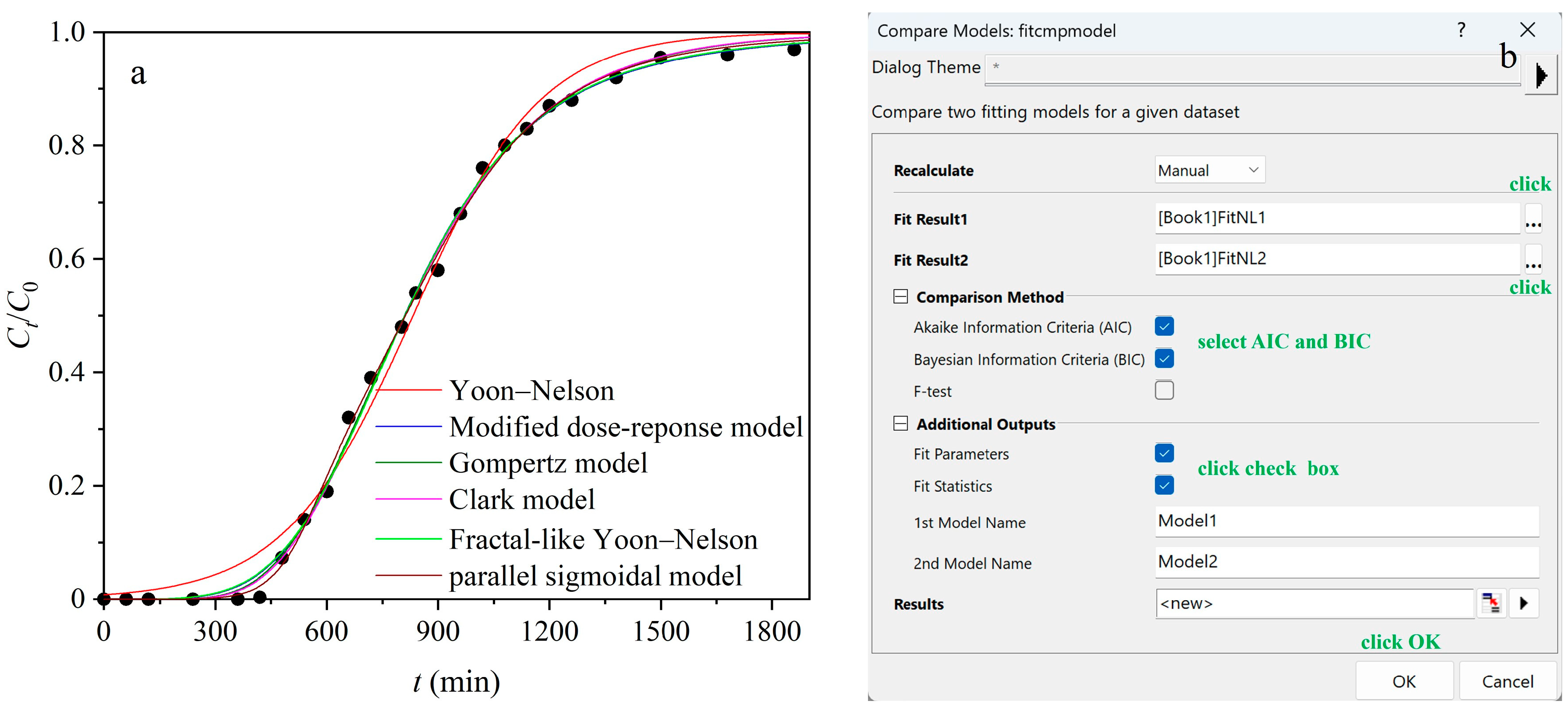
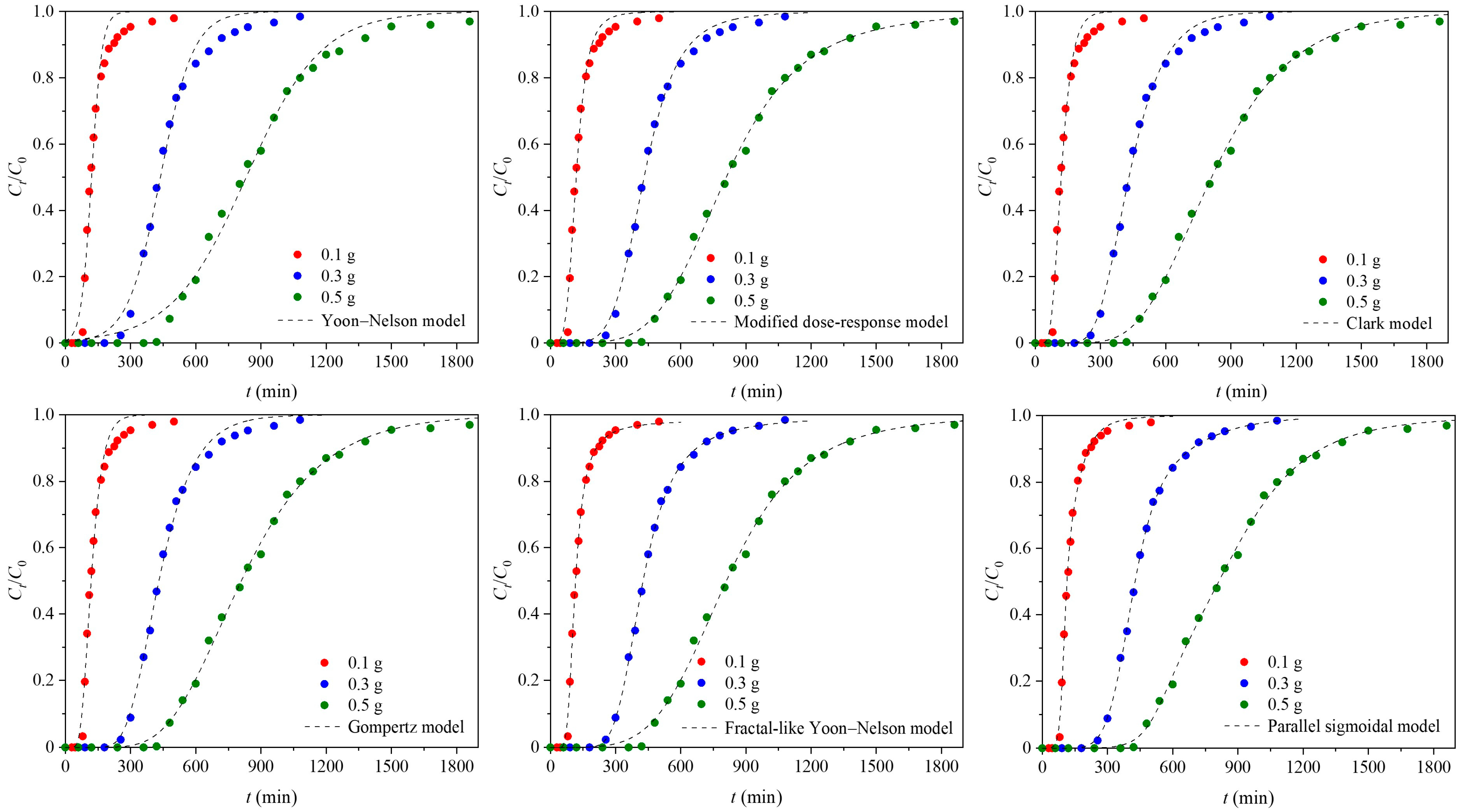
3.1. Empirical Breakthrough Models

3.1.1. Yoon–Nelson Model

Yoon and Nelson (1984) developed a model to describe gas– and liquid–solid adsorption [15]. The Yoon–Nelson model assumes that the rate of increase in the concentration of breakthrough is proportional to both the current concentration of breakthrough and the number of available active sites within the adsorbent bed.
C t C 0 = 1 1 + exp k YN τ t
It is important to note that the Yoon–Nelson model does not consider the characteristics of target contaminants, the type of the adsorbent and the physical properties of the column [16]. Thus, the Yoon–Nelson model is empirical to some extent, with parameters k YN and τ representing the lumped factors that encapsulate some physical processes and operating characteristics.

3.1.2. Modified Dose–Response Model

Given that the Thomas model offers a poor fit for the modeling of asymmetric breakthrough curves, Yan et al. (2001) derived the modified dose–response model to better describe heavy metal adsorption [13]. This model could well describe the asymmetric breakthrough curves, and the relative concentration ( C t / C 0 ) was equal to zero at the initial time (t = 0), which was written as
C t C 0 = 1 1 1 + v t b a

3.1.3. Gompertz Model

The measured breakthrough curves varied considerably across different adsorbent-adsorbate systems. In most cases, they were asymmetric for the adsorption of water contaminants [11]. This asymmetry was mainly attributed to three aspects [1]: (i) The intraparticle diffusion was the rate-limiting step, as was often the case in practice; (ii) The adsorbent consisted of multiple constituents with unequal reactivity; and (iii) The rate of adsorption declined more rapidly than the residual capacity of the adsorbent. Based on the Gompertz function, Hu et al. (2019) proposed a two-parameter empirical model to more reliably describe the asymmetric breakthrough curves [17], which is expressed as
C t C 0 = exp exp k τ t

3.1.4. Clark Model

The Clark model was originally used to evaluate the performance of granular activated carbon for the removal of low-concentration organic contaminants [12]. Its derivation was based on the combination of the mass-transfer concept with the Freundlich isotherm. The Clark model assumes that (i) An ideal plug flow takes place in the column; (ii) The film diffusion dominates during the adsorption processes; and (iii) The shape of the mass transfer zone remains unchanged. The Clark model also shows an asymmetric S-shaped curve, which is expressed as
C t C 0 = 1 1 + A exp r t 1 n 1
According to Equation (4), although the Clark model has a sound theoretical foundation, it does not directly provide the equilibrium loading, and its parameters A and r are lumped. These parameters are related to the mass-transfer coefficient and strongly depended on the operating conditions. Hence, the Clark model could be seen as a three-parameter empirical model in practice.

3.1.5. Fractal-like Yoon–Nelson Model

The adsorbent particles packed in the column are of energetically high heterogeneity due to the presence of pores with varying sizes and shapes (physical heterogeneity) and different functional groups on the solid surface (chemical heterogeneity) [18]. The assumption of a time-independent rate constant in such heterogeneous systems is often unsatisfactory for the explanation of diffusion-limited mass transfer processes [19]. As a result, the Yoon–Nelson model provides a poor fit for the modeling of breakthrough curves in some cases [20,21]. In contrast, the fractal-like theory assumes a temporal variation in the rate coefficient, providing new insights into dynamic adsorption behaviors [22]. This phenomenon could be expounded by the progressive occupation of the active sites with greater activation energies [23]. To this end, Hu et al. (2019) derived the fractal-like Yoon–Nelson model [10], which is expressed as
C t C 0 = 1 1 + exp k YN , 0 1 h τ 1 h t 1 h
Here, the parameter h represents a heterogeneity parameter related to the spectral dimension of fractal systems [24].

3.1.6. Parallel Sigmoidal Model

Blagojev et al. (2019) proposed the parallel sigmoidal model based on the observation that the breakthrough curves of Cu(II) adsorption are asymmetric under different operating conditions [25]. The model assumes that two kinds of adsorption sites are present on the adsorbent surface and that asymmetric breakthrough curves are caused by two distinct adsorption mechanisms that simultaneously occur on the adsorbent surface. The dominance of each mechanism changes over time. The parallel sigmoidal model is, essentially, the superposition of two modified dose–response models, which is expressed as
C t C 0 = p 1 1 1 + t τ 1 k 1 + 1 p 1 1 1 + t τ 2 k 2

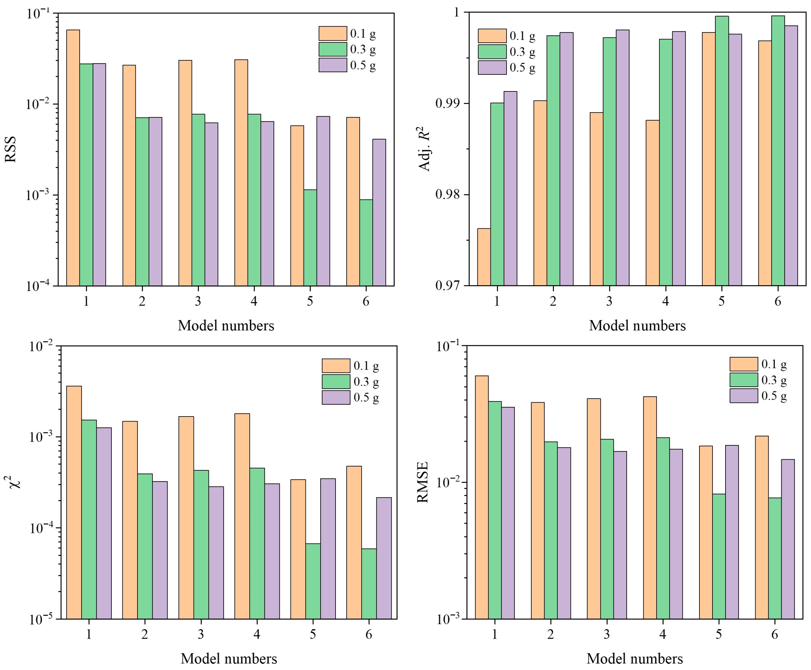
3.2. Fitting Quality

In the process of curve fitting, it was observed that six empirical models exhibited high fitting abilities. For this reason, the fitting of the breakthrough data by each model allowed for a clearer comparison between the fitted curves and the experimental data. One can readily see from Figure 2 that the measured breakthrough curves are asymmetric for all tested adsorbent masses (0.1, 0.3 and 0.5 g). The fitted curves generated by the Yoon–Nelson model deviate seriously from the data points, especially at the initial and final parts of the breakthrough curves. This discrepancy posed a challenge for the Yoon–Nelson model, as its fitting parameters failed to adequately explain the breakthrough behaviors. The Yoon–Nelson model is, mathematically, a logistic function, which inherently represents a symmetric S-shaped curve [1]. Thus, it provided a poor fit for the description of the measured breakthrough curves. In contrast, the modified dose–response and Gompertz models, despite having only two adjustable parameters, produced asymmetric function curves. This asymmetry allowed these two models to outperform the Yoon–Nelson model in terms of the fitting quality. In addition, the increase in the number of the model parameters generally contributed to improving the fitting ability. The Yoon–Nelson model could be regarded as a special case of the Clark model at n = 2. The adjustable parameter n in the Clark model provided greater flexibility during the curve fitting, making it more adaptable than the Yoon–Nelson model.
To further evaluate the fitting quality of these empirical models, four error statistics (RSS, Adj. R2, χ2 and RMSE) were used. As illustrated in Figure 3, the Clark model demonstrated a comparable performance to the modified dose–response and Gompertz models in terms of these error statistics. The fractal-like Yoon–Nelson model is optimal for the description of the breakthrough curve at the adsorbent mass of 0.1 g, as evidenced by the highest value of Adj. R2 and lowest values of RSS/RMSE/χ2 (see Table S1). Conversely, the parallel sigmoidal model yielded the best fit at adsorbent masses of 0.3 and 0.5 g.

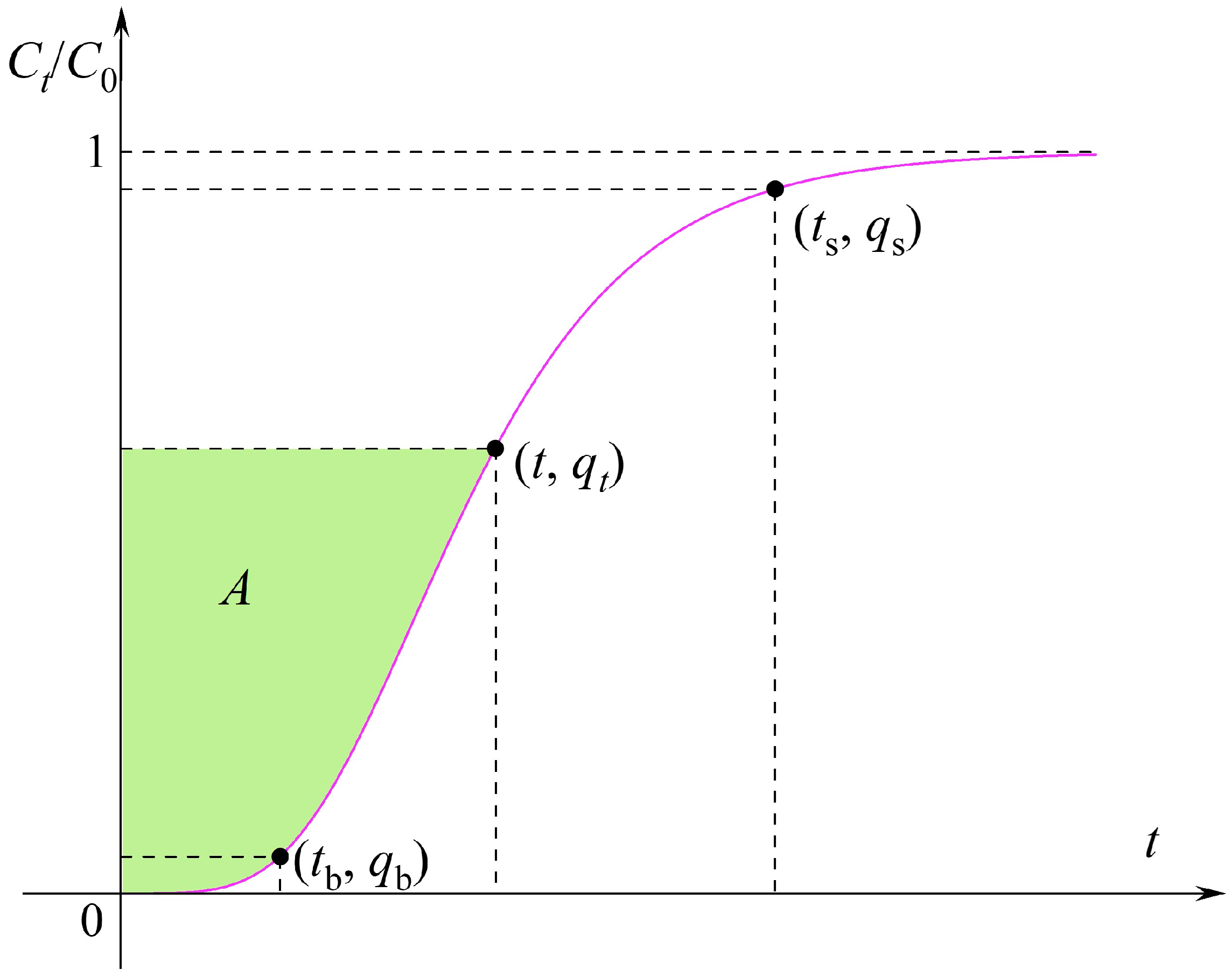
3.3. Equilibrium Loading

In view of the asymptotic property of the function curves provided by the above empirical models, the operating times required to reach 95% and 5% breakthrough in this study were defined as the saturation time ( t s , min) and the breakthrough time ( t b , min), respectively [1]. Since the roots of C t / C 0 = 0.95 or C t / C 0 = 0.05 were not easily determined for these six empirical models, it was crucial to develop a convenient method for calculating t s and t b . To achieve this, the roots were solved using the fzero command of MATLAB 2023b software. Although the equilibrium loading could not be directly obtained from the empirical models, it could be calculated by integrating the measured breakthrough curve [26]. As shown in Figure 4, the area (A) enclosed by the vertical axis, the horizontal line C t / C 0 = 1 and the measured breakthrough curve was numerically proportional to the average loading of the adsorbent bed at time t ( q t , mg g−1).
q t A = v C 0 A 1000 m = v C 0 1000 m 0 t 1 C t C 0 d t
Given that six empirical models considered in this study either lacked primitive functions or had primitives that were difficult to obtain, determining the definite integral in Equation (7) posed a significant challenge. To address this problem, we used the int command of MATLAB 2023b software to calculate the equilibrium loading ( q 0 , mg g−1), saturation capacity ( q s , mg g−1) and breakthrough capacity ( q b , mg g−1) at the total operating time ( t total , min), t s and t b , respectively. For example, the relevant MATLAB codes for the Yoon–Nelson model are provided in Appendix A, while the program codes for other empirical models are available in the Supplementary Materials.
As shown in Table 1, the values of q 0 , q s , q b , t s and t b vary significantly across different empirical models. According to the above fitting results, the equilibrium loading predicted by the fractal-like Yoon–Nelson model was 104.43 mg g−1 at the adsorbent mass of 0.1 g, while the equilibrium loadings predicted by the parallel sigmoidal model were 116.69 and 129.50 mg g−1 at adsorbent masses of 0.3 and 0.5 g.

3.4. Model Comparison

The error statistics could effectively measure how closely the fitted curve matched the measured breakthrough curves but could not compare models with different numbers of parameters. In general, the increase in the number of adjustable parameters contributed to promoting the fitting quality. In other words, the error statistics tended to favor the model with more parameters. However, this slight improvement in fitting quality was not enough to justify the increased model complexity. Hence, further comparison was necessary among these six models.
Recently, the Akaike information criterion (AIC) and Bayesian information criterion (BIC) have been widely used to balance the complexity and goodness of fit of models, which are expressed as [14]
AIC = n ln RSS n + 2 p
BIC = n ln RSS n + p ln n
where
RSS = i = 1 n y i y ' i 2
According to Equations (8) and (9), for a given set of breakthrough data, the value of n was fixed. The values of AIC and BIC decreased with the decrease in the value of RSS, indicating that the first term of AIC and BIC reflected the goodness of fit. Conversely, a larger value of p increased both the values of AIC and BIC and the model complexity. Therefore, the second term of AIC and BIC was often referred to as the penalty term. This penalty term helped to prevent overfitting by balancing the simplicity and accuracy of model comparison. The penalty term (pln(n)) of BIC contained the number of data points, making it stricter than that (2p) of AIC.
As shown in Figure 5, the parallel sigmoidal model exhibits the lowest value of AIC (−191.2) and the lowest value of BIC (−189.1). As a result, the adsorption of phosphate on the Ca-Fe-La composite followed the parallel sigmoidal model, which was consistent with the results indicated by the fitting curve and four error statistics. Accordingly, the predicted equilibrium loading was 129.50 mg g−1 at the adsorbent mass of 0.5 g.

4. Research Significance

The mathematical modeling of the breakthrough curves was crucial for understanding the dynamic adsorption behaviors in a fixed-bed column. The previous studies only focused on the fitting quality of empirical breakthrough models, ignoring their ability to explain the breakthrough behaviors. The adjustable parameters in these models were typically lumped or empirical, meaning that their values did not directly reflect the performance of the fixed-bed column. Thus, these empirical models were seen merely as mathematical tools for curve fitting rather than effective means for understanding the breakthrough behaviors. Based on the model parameters obtained by OriginPro 2021, this work adopted the int and fzero commands of MATLAB 2023b to successfully determine the parameters q 0 , q s , q b , t s and t b through writing the related program codes. These parameters further enabled the calculation of the length of the mass transfer zone and pollutant removal efficiency [27,28]. As mentioned above, the breakthrough curves were asymmetric in most cases. The Bohart–Adams and Thomas models had solid theoretical foundations, but they often gave a poor fit for the modeling of the measured breakthrough curves. The equilibrium loadings obtained from these two models failed to objectively reflect the performance of the fixed-bed column. In recent years, their applicability has been highly questioned. A previous study demonstrated that the Bohart–Adams, Thomas and Yoon–Nelson models are mathematically equivalent [10]. Therefore, aside from the Yoon–Nelson model, residual five empirical models were capable of describing the asymmetric breakthrough curves, thereby offering deeper insights into the breakthrough behaviors. The main significance of this study was its further promotion of the practical application of empirical breakthrough models.

5. Conclusions

In this study, the breakthrough time and saturation time were efficiently solved using the fzero command of MATLAB 2023b, while the equilibrium loading, breakthrough capacity and saturation capacity were determined by its int command. These process parameters were essential for evaluating the performance of the fixed-bed column. The Yoon–Nelson model provided a poor fit for the modeling of the breakthrough curves from phosphate adsorption on the Ca-Fe-La composite because of its symmetry. Error statistics and AIC/BIC analysis indicated that the parallel sigmoidal model was optimal. The predicted equilibrium loadings were 101.11, 116.69 and 129.50 mg g−1, respectively, at adsorbent masses of 0.1, 0.3 and 0.5 g. This study effectively bridged the gap between the undetermined parameters of empirical breakthrough models and the process parameters of the fixed-bed column, significantly enhancing their practical applicability.

Supplementary Materials

The following supporting information can be downloaded at: https://www.mdpi.com/article/10.3390/w17030329/s1, Table S1: Error statistics of six empirical models determined by OriginPro 2021 software.

Author Contributions

Q.H.: Conceptualization, investigation, formal analysis, data curation, project administration, writing—original draft, and visualization. Y.Z.: Conceptualization, formal analysis, writing—review and editing, supervision, project administration, and funding acquisition. Q.P.: formal analysis, data curation, and supervision. S.L.: data curation, writing—review and editing, and supervision. All authors have read and agreed to the published version of the manuscript.

Funding

This work was supported by Sichuan Science and Technology Program (No. 2024NSFSC0888, No. 2025YFHZ0269, No. 2025ZNSFSC0307), Yibin Scientific and Technology programs (No. SWJTU2021020007, No. SWJTU2021020008, No. YBSCXY2023020006, No. YBSCXY2023020007), Second Batch Talent Introduction Program of Sichuan University of Science & Engineering (No. 2024RC060, No. 2024RC099) and Sichuan Transportation Science and Technology Program (No. 2023-B-15).

Data Availability Statement

The data presented in this study are available on request from the corresponding author.

Conflicts of Interest

The authors declare no conflicts of interest.

Nomenclature

aempirical parameter in the modified dose–response model (a > 1)
AClark constant
bempirical parameter in the modified dose–response model (mL)
C 0 influent concentration (mg L−1)
C t effluent concentration at time t (mg L−1)
hfractal-like exponent
k YN Yoon–Nelson rate constant
k YN , 0 fractal-like Yoon–Nelson rate constant (min−(1−h))
k 1 empirical parameter in the parallel sigmoidal model
k 2 empirical parameter in the parallel sigmoidal model
nnumber of data points or Freundlich constant
mmass of the adsorbent packed in the column (g)
pproportion of each part in two-stage adsorption mechanism or number of the model parameters
q b breakthrough capacity (mg g−1)
q s saturation capacity (mg g−1)
q 0 equilibrium loading (mg g−1)
rClark constant (min−1)
toperating time (min)
t b breakthrough time (min)
t s saturation time (min)
t total total operating time (min)
vvolumetric flow rate (mL min−1)
y i observed values (y = Ct/C0)
ýipredicted values
χ2reduced chi-square
τoperating time required to reach 50% breakthrough (min)
τ 1 empirical parameter in the parallel sigmoidal model (min)
τ 2 empirical parameter in the parallel sigmoidal model (min)
RSSresidual sum of squares
Adj. R2adjusted coefficient of determination
RMSEroot of mean squared error
AICAkaike information criterion
BICBayesian information criterion

Appendix A

The model parameters were first determined by OriginPro 2021 at adsorbent masses of 0.1, 0.3 and 0.5 g, and then the parameters q 0 , q s , q b , t s and t b were calculated by MATLAB 2023b (see Supplementary Materials). The related program codes at an adsorbent mass of 0.1 g were as follows.
syms x;
a = 0.04155; % parameter kYN
b = 120.72059; % parameter τ
y = 1/(1 + exp(a*(b − x)));
f = @(x) 1/(1 + exp(a*(b − x))) − 0.05; % Definition of tb
t1 = fzero(f,50); % Initial value of tb was set as 50 and solution of tb
f = @(x) 1/(1 + exp(a*(b − x))) − 0.95; % Definition of ts
t2 = fzero(f,200); % Initial value of ts was set as 200 and solution of ts
c0 = 30; % initial phosphorus concentration of 30 mg L−1
v = 2.5; % flow rate of 2.5 mL min−1
m = 0.1; % adsorbent mass of 0.1 g
y1 = double(c0*v/(1000*m)*(int(1 − y, 0, t1))); % Solution of qb
y2 = double(c0*v/(1000*m)*(int(1 − y, 0, t2))); % Solution of qs
t3 = 500; % total operating time
y3 = double(c0*v/(1000*m)*(int(1 − y, 0, t3))); % Solution of q0

References

  1. Hu, Q.; Yang, X.; Huang, L.; Li, Y.; Hao, L.; Pei, Q.; Pei, X. A critical review of breakthrough models with analytical solutions in a fixed-bed column. J. Water Process Eng. 2024, 59, 105065. [Google Scholar] [CrossRef]
  2. Juela, D.; Vera, M.; Cruzat, C.; Astudillo, A.; Vanegas, E. A new approach for scaling up fixed-bed adsorption columns for aqueous systems: A case of antibiotic removal on natural adsorbent. Process Saf. Environ. Prot. 2022, 159, 953–963. [Google Scholar] [CrossRef]
  3. Taka, A.L.; Klink, M.J.; Mbianda, X.Y.; Naidoo, E.B. Chitosan nanocomposites for water treatment by fixed-bed continuous flow column adsorption: A review. Carbohydr. Polym. 2021, 255, 117398. [Google Scholar] [CrossRef]
  4. Worch, E. Adsorption Technology in Water Treatment: Fundamentals, Processes, and Modeling; Walter de Gruyter GmbH & Co KG: Berlin, Germany, 2012. [Google Scholar]
  5. Suzaki, P.Y.R.; Munaro, M.T.; Triques, C.C.; Kleinübing, S.J.; Klen, M.R.F.; Bergamasco, R.; de Matos Jorge, L.M. Phenomenological mathematical modeling of heavy metal biosorption in fixed-bed columns. Chem. Eng. J. 2017, 326, 389–400. [Google Scholar] [CrossRef]
  6. Suzaki, P.Y.R.; Triques, C.C.; Munaro, M.T.; Steffen, V.; Kleinübing, S.J.; Klen, M.R.F.; Bergamasco, R.; de Matos Jorge, L.M. Phenomenological modeling and simulation of competitive biosorption of ternary heavy metal systems in a fixed bed column. Chem. Eng. Res. Des. 2023, 196, 701–710. [Google Scholar] [CrossRef]
  7. Hamdaoui, O. Removal of copper(II) from aqueous phase by Purolite C100-MB cation exchange resin in fixed bed columns: Modeling. J. Hazard. Mater. 2009, 161, 737–746. [Google Scholar] [CrossRef]
  8. Bohart, G.S.; Adams, E.Q. Some aspects of the behavior of charcoal with respect to chlorine. J. Am. Chem. Soc. 1920, 42, 523–544. [Google Scholar] [CrossRef]
  9. Thomas, H.C. Chromatography: A problem in kinetics. Ann. N. Y. Acad. Sci. 1948, 49, 161–182. [Google Scholar] [CrossRef]
  10. Hu, Q.; Xie, Y.; Feng, C.; Zhang, Z. Fractal-like kinetics of adsorption on heterogeneous surfaces in the fixed-bed column. Chem. Eng. J. 2019, 358, 1471–1478. [Google Scholar] [CrossRef]
  11. Rojas-Mayorga, C.K.; Bonilla-Petriciolet, A.; Sánchez-Ruiz, F.J.; Moreno-Pérez, J.; Reynel-Ávila, H.E.; Aguayo-Villarreal, I.A.; Mendoza-Castillo, D.I. Breakthrough curve modeling of liquid-phase adsorption of fluoride ions on aluminum-doped bone char using micro-columns: Effectiveness of data fitting approaches. J. Mol. Liq. 2015, 208, 114–121. [Google Scholar] [CrossRef]
  12. Clark, R.M. Evaluating the cost and performance of field-scale granular activated carbon systems. Environ. Sci. Technol. 1987, 21, 573–580. [Google Scholar] [CrossRef]
  13. Yan, G.; Viraraghavan, T.; Chen, M. A new model for heavy metal removal in a biosorption column. Adsorpt. Sci. Technol. 2001, 19, 25–43. [Google Scholar] [CrossRef]
  14. Hu, Q.; He, Z.; Zhang, Y.; Ma, S.; Huang, L. One-pot solvothermal synthesis of Ca-Fe-La composite for advanced removal of phosphate from aqueous solutions in a fixed-bed column: Modeling and resource utilization. Environ. Technol. Innov. 2024, 36, 103888. [Google Scholar] [CrossRef]
  15. Yoon, Y.H.; Nelson, J.H. Application of gas adsorption kinetics I. A theoretical model for respirator cartridge service life. Am. Ind. Hyg. Assoc. J. 1984, 45, 509–516. [Google Scholar] [CrossRef]
  16. Tejedor, J.; Álvarez-Briceño, R.; Guerrero, V.H.; Villamar-Ayala, C.A. Removal of caffeine using agro-industrial residues in fixed-bed columns: Improving the adsorption capacity and efficiency by selecting adequate physical and operational parameters. J. Water Process. Eng. 2023, 53, 103778. [Google Scholar] [CrossRef]
  17. Hu, Q.; Xie, Y.; Feng, C.; Zhang, Z. Prediction of breakthrough behaviors using logistic, hyperbolic tangent and double exponential models in the fixed-bed column. Sep. Purif. Technol. 2019, 212, 572–579. [Google Scholar] [CrossRef]
  18. Wang, Y.; Wang, C.; Huang, X.; Zhang, Q.; Wang, T.; Guo, X. Guideline for modeling solid-liquid adsorption: Kinetics, isotherm, fixed bed, and thermodynamics. Chemosphere 2024, 349, 140736. [Google Scholar] [CrossRef]
  19. Kopelman, R. Fractal reaction kinetics. Science 1988, 241, 1620–1626. [Google Scholar] [CrossRef]
  20. de Oliveira, J.T.; Costa, L.R.D.C.; Agnol, G.D.; Féris, L.A. Experimental design and data prediction by Bayesian statistics for adsorption of tetracycline in a GAC fixed-bed column. Sep. Purif. Technol. 2023, 319, 124097. [Google Scholar] [CrossRef]
  21. Jiang, S.; Lyu, Y.; Zhang, J.; Zhang, X.; Yuan, M.; Zhang, Z.; Jin, G.; He, B.; Xiong, W.; Yi, H. Continuous adsorption removal of organic pollutants from wastewater in a UiO-66 fixed bed column. J. Environ. Chem. Eng. 2024, 12, 111951. [Google Scholar] [CrossRef]
  22. Montagnaro, F.; Balsamo, M. Modelling CO2 adsorption dynamics onto amine-functionalised sorbents: A fractal-like kinetic perspective. Chem. Eng. Sci. 2018, 192, 603–612. [Google Scholar] [CrossRef]
  23. Haerifar, M.; Azizian, S. Fractal-like kinetics for adsorption on heterogeneous solid surfaces. J. Phys. Chem. C 2014, 118, 1129–1134. [Google Scholar] [CrossRef]
  24. Balsamo, M.; Montagnaro, F. Liquid–solid adsorption processes interpreted by fractal-like kinetic models. Environ. Chem. Lett. 2019, 17, 1067–1075. [Google Scholar] [CrossRef]
  25. Blagojev, N.; Kukić, D.; Vasić, V.; Šćiban, M.; Prodanović, J.; Bera, O. A new approach for modelling and optimization of Cu(II) biosorption from aqueous solutions using sugar beet shreds in a fixed-bed column. J. Hazard. Mater. 2019, 363, 366–375. [Google Scholar] [CrossRef]
  26. Mendes, P.A.P.; Rodrigues, A.E.; Horcajada, P.; Serre, C.; Silva, J.A.C. Single and multicomponent adsorption of hexane isomers in the microporous ZIF-8. Microporous Mesoporous Mater. 2014, 194, 146–156. [Google Scholar] [CrossRef]
  27. Nordin, A.H.; Ngadi, N.; Nordin, M.L.; Noralidin, N.A.; Nabgan, W.; Osman, A.Y.; Shaari, R. Spent tea waste extract as a green modifying agent of chitosan for aspirin adsorption: Fixed-bed column, modeling and toxicity studies. Int. J. Biol. Macromol. 2023, 253, 126501. [Google Scholar] [CrossRef]
  28. Najafi, H.; Maklavani, N.A.; Asasian-Kolur, N.; Sharifian, S.; Harasek, M. Copper oxide-incorporated pillared clay granular nanocomposite for efficient single and binary, batch and fixed bed column adsorption of levofloxacin and crystal violet. Chem. Eng. Sci. 2024, 295, 120184. [Google Scholar] [CrossRef]
Figure 1. (a) Fitting results of six empirical models, (b) determination of AIC and BIC in the Compare Models: fitcmpmodel dialog box.
Water 17 00329 g001
Figure 2. Fitting results of six empirical models for phosphate adsorption on the Ca-Fe-La composite.
Water 17 00329 g002
Figure 3. Error statistics for various empirical models (1: Yoon–Nelson model, 2: modified dose–response model, 3: Gompertz model, 4: Clark model, 5: fractal-like Yoon–Nelson model, 6: parallel sigmoidal model).
Water 17 00329 g003
Figure 4. Schematic diagram of the average loading of the adsorbent bed at time t.
Water 17 00329 g004
Figure 5. Model comparison: (a) AIC, (b) BIC (1: Yoon–Nelson model, 2: modified dose–response model, 3: Gompertz model, 4: Clark model, 5: fractal-like Yoon–Nelson model, 6: parallel sigmoidal model).
Water 17 00329 g005
Table 1. Related parameters obtained by OriginPro 2021 and MATLAB 2023b software.
m (g)Yoon–Nelson modelqb (mg g−1)tb (min)qs (mg g−1)ts (min)q0 (mg g−1)
kYN (min−1)τ (min)
0.14.12 × 10−2120.736.5949.989.73191.690.66
0.31.32 × 10−2437.452.46213.5108.44661.3109.41
0.55.80 × 10−3832.147.55324.4123.701339.8124.96
m (g)Modified dose–response modelqb (mg g−1)tb (min)qs (mg g−1)ts (min)q0 (mg g−1)
ab (mL)
0.14.620296.746.6462.893.88224.596.14
0.35.5271078.762.83253.3111.82735.1113.54
0.54.6192023.563.60427.9128.031531.0129.66
m (g)Gompertz modelqb (mg g−1)tb (min)qs (mg g−1)ts (min)q0 (mg g−1)
k (min−1)τ (min)
0.12.81 × 10−2105.849.6566.793.40211.694.75
0.38.99 × 10−3389.966.60267.9112.12720.3113.48
0.53.96 × 10−3717.165.50440.00127.501467.1129.01
m (g)Clark modelqb (mg g−1)tb (min)qs (mg g−1)ts (min)q0 (mg g−1)
Ar (min−1)n
0.11.64 × 10−22.87 × 10−21.000850.9968.493.83210.395.15
0.31.30 × 10−28.99 × 10−31.000466.71268.3112.24720.8113.59
0.51.09 × 10−24.01 × 10−31.000666.72448.1127.981462.6129.48
m (g)Fractal-like Yoon–Nelson modelqb (mg g−1)tb (min)qs (mg g−1)ts (min)q0 (mg g−1)
kYN,0 (min−(1−h))τ (min)h
0.1895.3115.82.09254.7873.499.24298.6104.43
0.3930.1426.81.83969.52279.5114.74827.5116.88
0.53.505810.30.95963.10424.7127.841520.5129.48
m (g)Parallel sigmoidal modelqb (mg g−1)tb (min)qs (mg g−1)ts (min)q0 (mg g−1)
k1 (min)τ1 (min)k2 (min−1)τ2 (min)p
0.18.916101.84.097158.80.55955.2174.198.20262.5101.11
0.36.909411.15.257736.20.87367.94273.5114.86834.3116.69
0.59.606572.55.378900.40.22669.61467.0127.851480.2129.50
Disclaimer/Publisher’s Note: The statements, opinions and data contained in all publications are solely those of the individual author(s) and contributor(s) and not of MDPI and/or the editor(s). MDPI and/or the editor(s) disclaim responsibility for any injury to people or property resulting from any ideas, methods, instructions or products referred to in the content.

