1. Introduction
High arch dams, as the core infrastructures of hydropower stations, are pivotal to sustainable water resource utilization, clean energy production, and downstream flood mitigation [
1]. These large-scale concrete structures are subjected to complex service environments and must operate reliably over long time spans. The structural integrity of such dams is critical, as any failure could result in severe socioeconomic and environmental consequences [
2,
3]. The deformation behavior of high arch dams is influenced by a combination of interacting factors, including hydrostatic loading from reservoir level fluctuations, thermally induced stress variations, site-specific geological conditions, and external disturbances such as earthquakes or extreme precipitation events.
Conventional safety assessment approaches, such as empirical threshold-based methods and shallow machine learning models, often struggle with the effective processing and interpretation of complex monitoring data, failing to accurately capture the inherent nonlinearities, spatiotemporal dependencies, and dynamic hydraulic responses associated with dam and hydraulic station deformation processes [
4,
5,
6].
To monitor the structural health and operational safety of hydropower stations under such complex influences, comprehensive safety monitoring systems are typically deployed [
7,
8,
9,
10,
11,
12]. These structural monitoring systems collect a wide range of prototypical data, including displacement measurements, water pressure readings, temperature profiles, and other critical indicators, providing essential inputs for the assessment of dam behavior and the early detection of potential anomalies. For instance, Cao et al. [
13] proposed a spatiotemporal clustering and zonal prediction approach for super-high arch dam deformation analysis by combining CFSFDP-based clustering of measurement points with a STARIMA-based spatiotemporal modeling framework. Chen et al. [
5] developed a feature decomposition-based deep transfer learning framework (FD-DTL) that integrates VMD, DE, MIC, and TL-CNN-LSTM modeling to enable accurate concrete dam deformation prediction under observational insufficiency by leveraging knowledge transfer from similar feature components across dams. Tian et al. [
14] proposed a deep transfer learning-based time-varying deformation monitoring model for high earth-rock dams, which combines GCN-LSTM and attention mechanisms with starting point time markers to enhance prediction accuracy and generalization under time-varying nonlinear deformation behaviors. These studies collectively demonstrate the notable advantages of deep learning (DL) approaches in dam displacement forecasting, particularly in their capacity to capture complex nonlinearities, temporal dependencies, and spatial correlations inherent in dam behavior. However, given the increasing availability of long-term, high-dimensional monitoring data from modern dam safety systems, there remains a critical need for further research focused on the design of neural network architectures that can efficiently handle long-sequence, multi-variable monitoring data while maintaining robustness and interpretability.
With the advent of high-frequency, multi-dimensional monitoring data (e.g., displacement, seepage pressure, temperature), there is a need for models that can capture both spatial patterns and temporal dynamics [
15,
16,
17,
18]. In response, artificial intelligence (AI) technologies, particularly deep learning (DL) methods, have emerged as powerful tools for mining complex relationships hidden within monitoring data [
19,
20,
21,
22,
23]. For example, Convolutional Neural Networks (CNNs) have demonstrated strong capabilities in extracting spatial features from structured and unstructured monitoring datasets [
24], while Long Short-Term Memory (LSTM) networks excel at modeling long-term temporal dependencies, making them highly suitable for time-series forecasting tasks in dam deformation analysis [
25]. By leveraging such AI-driven approaches, it becomes possible to enhance the predictive accuracy, adaptiveness, and robustness of dam safety evaluation systems under varying hydraulic and environmental conditions.
Building upon these advancements, recent studies have begun exploring hybrid architectures that integrate CNNs with recurrent neural networks to simultaneously learn spatial–temporal representations [
11,
12,
18,
26]. While CNN–LSTM frameworks have shown promise in dam displacement prediction, they often suffer from high computational costs and limited training efficiency due to the complex gating mechanisms of LSTMs.
To address these limitations, this study develops an optimized CNN–GRU model for displacement prediction of hydraulic stations that couples CNN’s spatial feature extraction with the Gated Recurrent Unit (GRU)’s simplified yet effective temporal modeling capability. The CNN component is employed to extract spatial features from multi-dimensional monitoring data, while the GRU component effectively captures temporal dependencies with a more concise structure compared to LSTM. This hybrid design not only reduces model complexity and training time but also improves prediction accuracy and robustness, making it well-suited for long-sequence monitoring data in high arch dam safety evaluation. Compared with traditional CNN–LSTM structures, the proposed CNN–GRU framework achieves faster convergence, reduced parameter complexity, and improved forecasting accuracy, thereby providing a more efficient and reliable tool for intelligent displacement monitoring and safety assessment of hydropower stations.
2. Methods
2.1. Convolutional Architecture
The Gated Recurrent Unit (GRU) is a widely used variant of recurrent neural networks (RNNs) designed to effectively model sequential data by addressing the vanishing gradient problem inherent in traditional RNN architectures [
27]. By incorporating gating mechanisms, specifically the update gate and reset gate, GRUs can adaptively control the flow of information through the network, thereby capturing long-term temporal dependencies with relatively low computational complexity. Compared to Long Short-Term Memory (LSTM) networks, GRUs offer a more lightweight structure with fewer parameters, making them advantageous for modeling time series data with limited computational resources. However, despite their effectiveness in capturing temporal dynamics, conventional GRUs exhibit certain limitations when applied to complex real-world monitoring data in hydraulic structures.
Figure 1 shows the schematic diagram of the convolutional neural network. Specifically, traditional GRUs often lack the capacity to directly exploit spatial correlations inherent in multi-point monitoring systems, as they primarily focus on one-dimensional temporal sequences. Moreover, without explicit spatial feature extraction, GRUs may struggle to accurately represent the intricate spatiotemporal interactions that are critical for detecting subtle structural anomalies under varying hydraulic loading conditions. These limitations highlight the need for hybrid architectures that integrate spatial modeling capabilities, such as Convolutional Neural Networks (CNNs), with temporal sequence learning, to enhance predictive performance in dam safety monitoring applications.
2.2. Stacked GRU Model
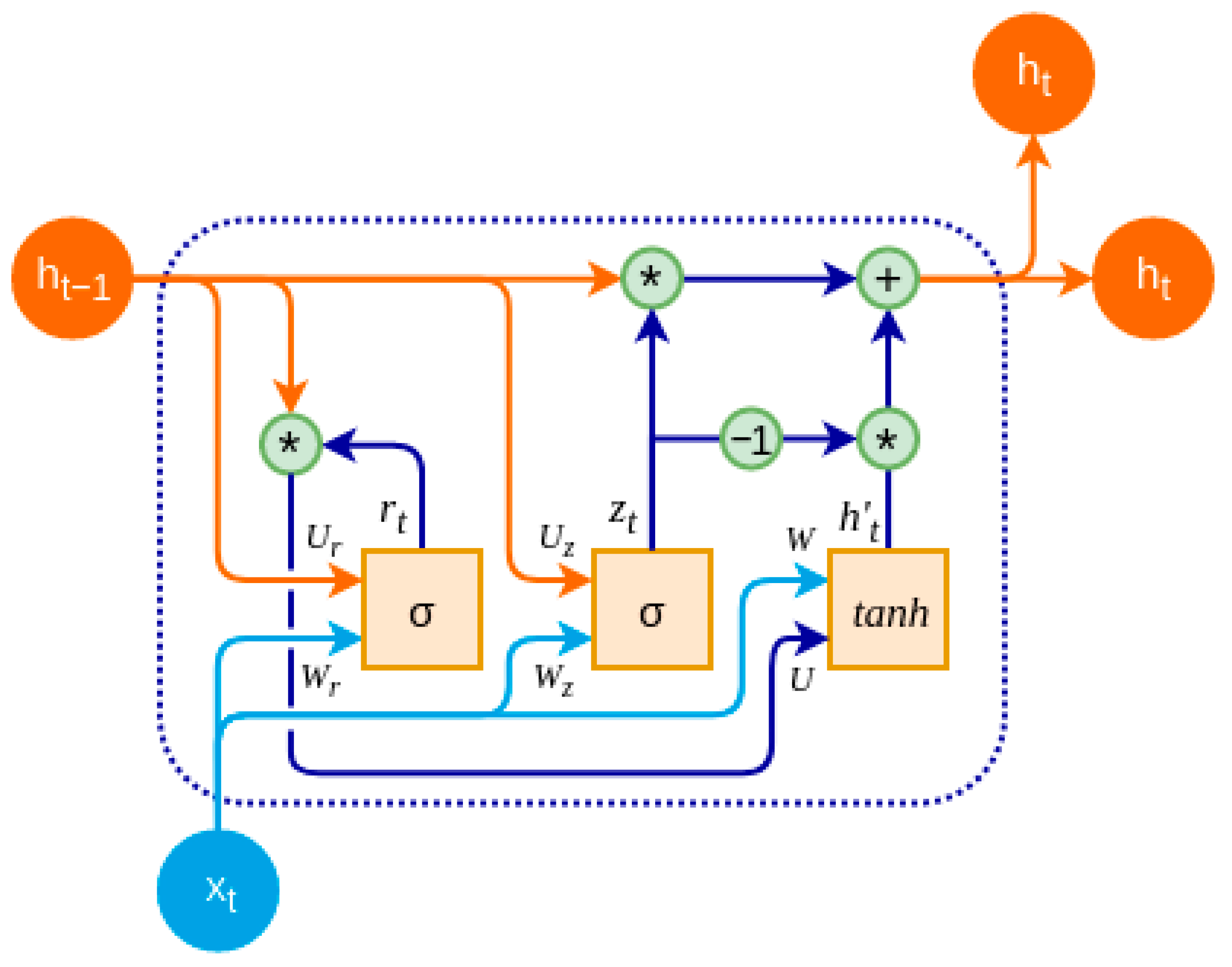
The Gated Recurrent Unit (GRU) is a variant of recurrent neural networks (RNNs) designed to efficiently capture long-term temporal dependencies while mitigating the vanishing gradient problem. Compared to the traditional Long Short-Term Memory (LSTM) network, GRU features a more compact architecture with fewer parameters, resulting in improved computational efficiency without sacrificing modeling capability. The overall architecture of the GRU network is illustrated in
Figure 2, which highlights its key components, including the update and reset gates, that enable the selective control of information flow and memory retention across time steps.
In this study, a stacked GRU architecture is employed to enhance the temporal feature extraction capability for long-sequence deformation prediction. A diagram of the CNN-multi-stacked-GRU network can be seen in
Figure 3. The model comprises multiple GRU layers arranged in a hierarchical manner, where the output sequence from one GRU layer serves as the input for the subsequent layer. This stacked configuration enables the model to learn increasingly abstract representations of temporal patterns over deeper levels, improving its ability to model complex, nonlinear dependencies in the monitoring data.
The input to the stacked GRU model consists of multivariate time series data, including environmental variables (e.g., temperature, reservoir level) and historical deformation measurements. Through layer-wise recurrent processing, the model effectively captures both short-term fluctuations and long-term trends, which are critical for accurate deformation forecasting in hydropower station structures.
2.3. Adaptive Inertia Weight PSO (AIW-PSO)Algorithm
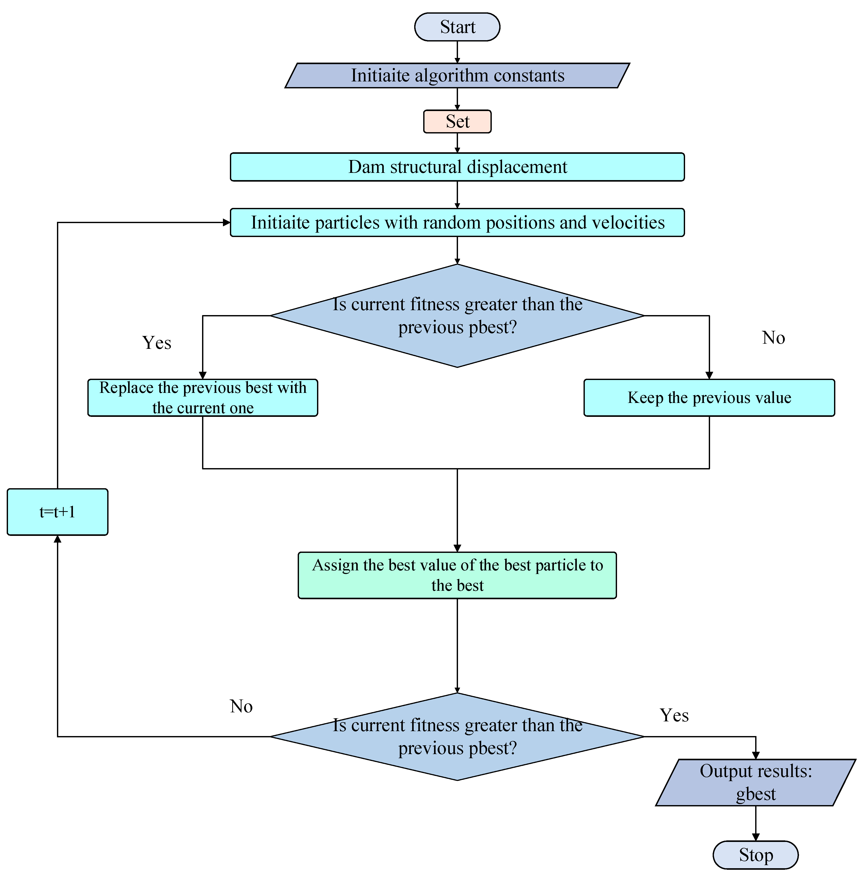
To optimize the hyperparameters of the proposed CNN-stacked-GRU framework, an improved Particle Swarm Optimization (PSO) algorithm with adaptive inertia weight adjustment was employed.
Figure 4 shows the schematic diagram of the improved PSO algorithm. Unlike standard PSO, the improved PSO dynamically adjusts the inertia weight during the optimization process, enabling a better balance between global exploration and local exploitation.
Figure 5 shows the parameter optimization process based on improved PSO and deep neural networks. At the early stages of the search, a larger inertia weight encourages particles to explore the hyperparameter space more broadly, reducing the likelihood of premature convergence. As the iteration progresses, the inertia weight decreases, enhancing the fine-tuning capability around promising regions. This adaptive strategy significantly improves optimization stability and solution quality, particularly in the highly nonlinear and dynamic modeling environment of the dam and hydraulic station monitoring data.
2.4. Evaluation Metrics
To evaluate the classification performance of the proposed model, three commonly used metrics, including Accuracy, F1-score, and False Positive Rate (FPR), are adopted. Accuracy reflects the overall proportion of correctly classified instances and provides a general measure of model performance. F1-score, as the harmonic mean of precision and recall, offers a balanced evaluation, particularly important when dealing with imbalanced data. Together, these metrics enable a comprehensive assessment of the model’s effectiveness in crack identification tasks.
3. Case Study
3.1. Project Description
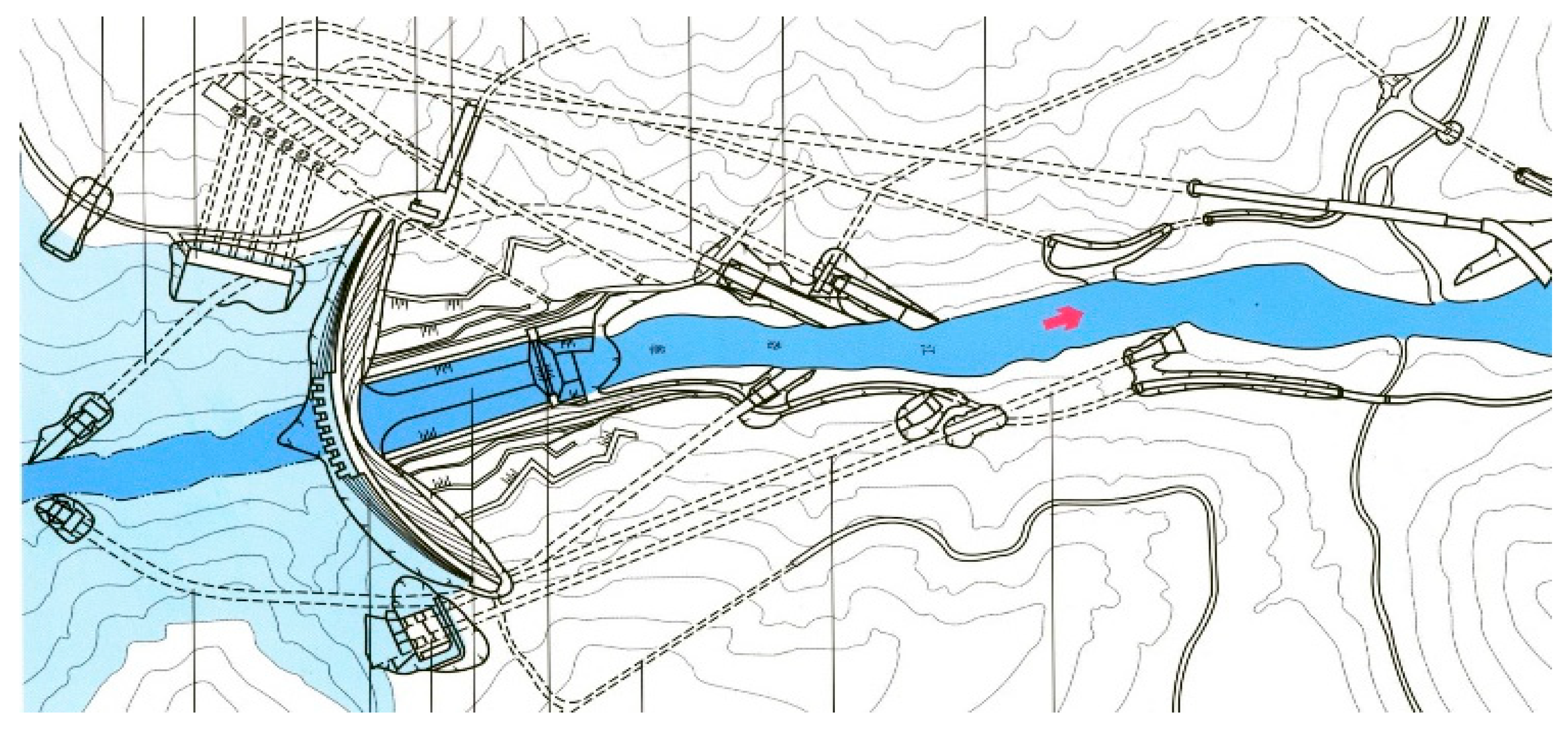
The investigated concrete arch dam has a maximum height of 280 m and is divided into multiple structural sections. The hydraulic station is an annual regulating reservoir, and its plan layout is shown in
Figure 6 and
Figure 7. The dam body incorporates an internal system comprising approximately 100 horizontal galleries, 20 foundation galleries, and 100 branch galleries, which facilitate inspection, drainage, and structural monitoring. The reservoir is primarily intended for hydropower generation, operating at a normal water level of 1200 m and providing a total storage capacity of about 1 × 10
8 m
3.
3.2. Environmental Monitoring Data Visualization and Statistical Analysis
Figure 8 presents the time-series trends and corresponding statistical distributions of three key hydraulic variables, including the upstream water height, downstream water height, and rainfall, monitored continuously at the hydraulic station over an extended period. The process lines (
Figure 8a–c) reveal distinct temporal dynamics: the upstream water height exhibits pronounced cyclical fluctuations driven by seasonal hydrological patterns and reservoir operation schedules, while the downstream water height shows more irregular short-term variations, primarily governed by discharge control and downstream hydraulic responses. In contrast, rainfall displays highly intermittent behavior, characterized by sporadic high-intensity precipitation events interspersed with prolonged dry periods. The distribution plots (
Figure 8d–f) further elucidate these patterns. The upstream water height exhibits a bimodal distribution, reflecting frequent transitions between typical operational levels and drawdown conditions. The downstream water height follows a moderately skewed distribution centered around 40–42 m, indicative of relatively stable flow regulation. Rainfall distribution is markedly right-skewed, with a high concentration of low or zero-rainfall occurrences and occasional extreme events.
In this study, ten temperature sensors (T1–T10) were deployed at three representative sections of the high arch dam, Sections 11, 20, and 32, at multiple elevations within each section to capture vertical thermal gradients. The arrangement was designed to measure distinct thermal conditions, with dedicated sensors for water temperature, air temperature, and concrete temperature.
Figure 9 illustrates the long-term time-series trends of the ten temperature sensors deployed within this hydropower station. The sensors exhibit distinct thermal behaviors depending on their spatial locations. Sensors such as Sensor01, Sensor02, Sensor03, Sensor09, and Sensor10 display strong seasonal variations with large temperature amplitudes, reflecting their exposure to external environmental conditions or dynamic hydraulic zones. In contrast, sensors such as Sensor05, Sensor06, and Sensor08 show relatively stable temperature profiles, indicating deployment in thermally insulated or less exposed structural regions.
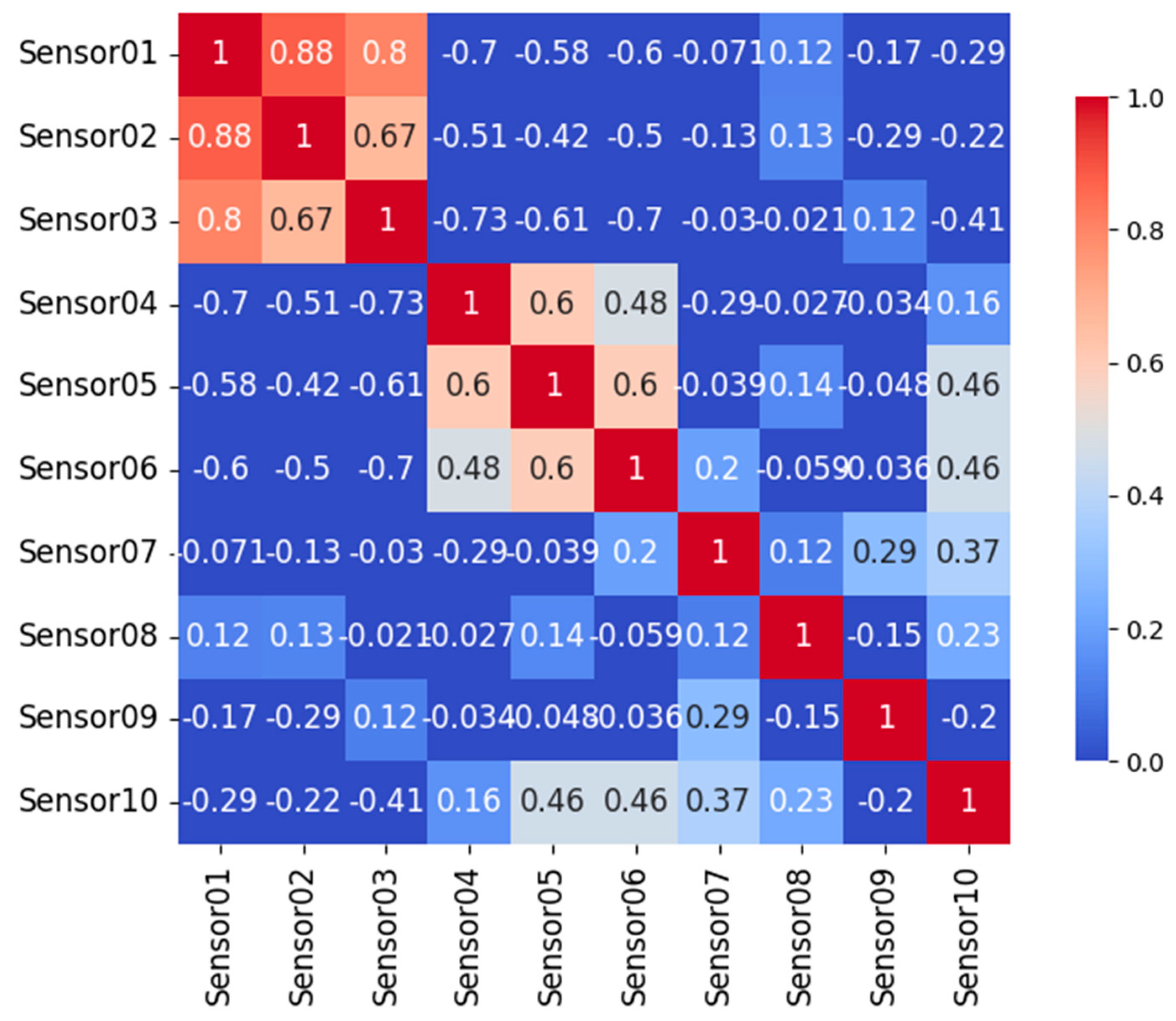
Figure 10 presents the correlation matrix of these temperature sensors. Strong positive correlations are observed among sensors with similar thermal exposure (e.g., Sensor01, Sensor02, and Sensor03), suggesting coherent thermal responses driven by shared environmental influences. In contrast, weaker or negative correlations are observed between sensors located in thermally decoupled regions (e.g., between Sensor01 and Sensor05–Sensor08), highlighting the spatial heterogeneity of the temperature field within the structure. The combination of the time-series and correlation analyses underscores the importance of considering both spatial sensor placement and local thermal conditions when interpreting temperature effects in structural health monitoring and deformation modeling.
3.3. Statistical Analysis of Displacement Time Series Data
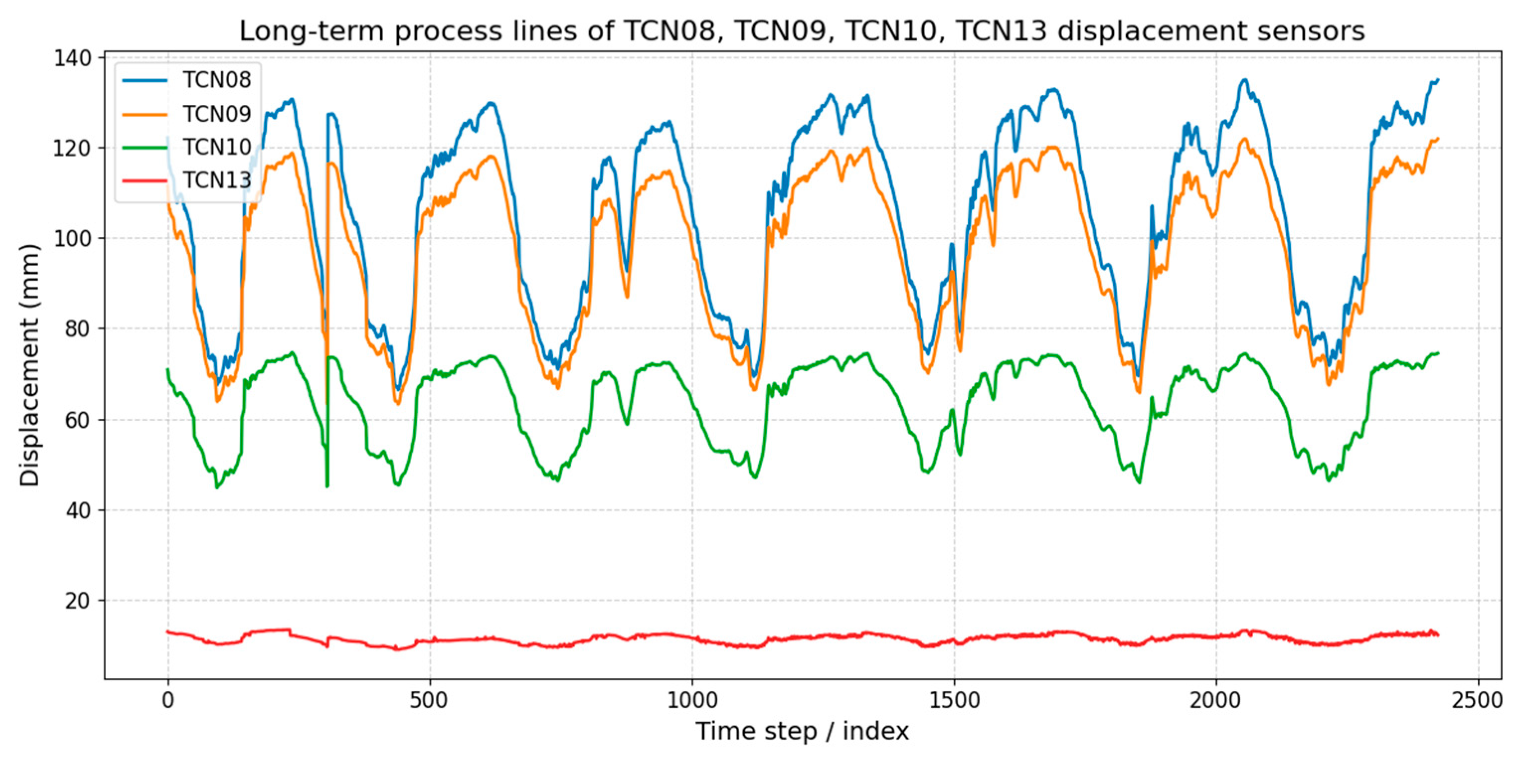
The visualization results of the dam displacement monitoring data can be seen in
Figure 11. The long-term displacement records of these dam displacement sensors exhibit distinct temporal patterns with clear seasonal cycles and varying amplitudes. TCN08 and TCN09 show the largest displacements, ranging approximately between 90 and 140 mm, and are highly correlated in both magnitude and trend, suggesting that they are located in structurally similar positions. TCN10 displays lower amplitudes (50–80 mm) but still follows the same periodic fluctuation, indicating a consistent thermal or environmental influence across the monitoring system. In contrast, TCN13 remains nearly flat around 10–15 mm with minimal variation, reflecting either a structurally more stable position or reduced sensitivity to the external loading conditions. Overall, the results demonstrate spatial variability in structural response, where the relative magnitude and periodicity of displacement provide insights into both local boundary conditions and global deformation mechanisms.
The displacement distributions of the four sensors can be seen in
Figure 12, demonstrating significant variability in both range and central tendency. TCN08 and TCN09 exhibit broad distributions with higher displacement values, typically centered between 110 and 130 mm, indicating larger structural movement at their locations. TCN10 shows a narrower distribution within the 50–75 mm range, reflecting comparatively moderate displacement behavior. In contrast, TCN13 remains tightly clustered around 10–13 mm, suggesting that it experiences minimal deformation and is located in a structurally more stable region. The distinct differences in distribution among the sensors highlight the spatial heterogeneity of displacement responses, which may be attributed to varying boundary conditions, loading effects, or structural constraints at the monitored points.
4. Experimental Result Analysis and Discussion
The experiments were implemented on a personal workstation equipped with an Intel Core i7-11700 CPU and an NVIDIA GeForce RTX 3060 GPU with 12 GB of memory. The system was configured with 32 GB of RAM and operated under Windows 10. The models were developed in Python 3.9 using the PyTorch 1.12 framework, with CUDA 11.3 for GPU acceleration. Data preprocessing and result visualization were carried out using standard scientific libraries, including NumPy 2.1.3, pandas 2.2.3, and Matplotlib 3.9.2.
4.1. Model Hyperparameter Optimization and Training
The developed CNN–GRU model for dam deformation prediction was trained using long-sequence monitoring data collected from the hydropower station. A total of 40 input factors were incorporated, covering hydrological, meteorological, and environmental conditions, such as reservoir water level, rainfall, and air temperature. The dam displacement served as the target output variable. Prior to training, all input features were standardized to zero mean and unit variance in order to accelerate convergence and ensure numerical stability. To preserve the temporal dependencies intrinsic to the monitoring data, the dataset was partitioned into training, validation, and testing subsets in a chronological manner, following a standard ratio of 70:15:15. The CNN layers were first applied to extract local spatial patterns from multivariate time series input windows. The resulting feature maps were then fed into stacked GRU layers to learn temporal dependencies over long observation periods. The model was trained using the Adam optimizer with an initial learning rate of 0.001. A mean squared error (MSE) loss function was used to quantify the prediction error between the model output and the actual displacement measurements.
To prevent overfitting, early stopping was implemented based on the validation loss with a patience of 20 epochs. Dropout regularization and L2 weight decay were also applied during training. The optimal model configuration, including the number of convolutional filters, GRUs, and sequence length, was determined through a hyperparameter optimization process described in
Section 4.2. All training procedures were conducted using PyTorch on a GPU-accelerated computing platform to ensure computational efficiency.
The training loss curve of the proposed CNN-GRU model can be seen in
Figure 13, demonstrating a clear convergence trend over 200 epochs. Initially, the loss decreases sharply in the proposed method sharply during the first 20–30 epochs, indicating that the model rapidly captures the underlying patterns in the training data. As training progresses, the rate of loss reduction gradually diminishes, and from approximately epoch 50 onwards, the loss stabilizes at a low value close to zero. This behavior reflects effective learning dynamics, where the model transitions from coarse to fine adjustments of its parameters. The smooth and consistent decline without significant oscillations further suggests that the chosen network architecture and hyperparameter configuration provide stable training and good convergence properties, with no evident signs of overfitting.
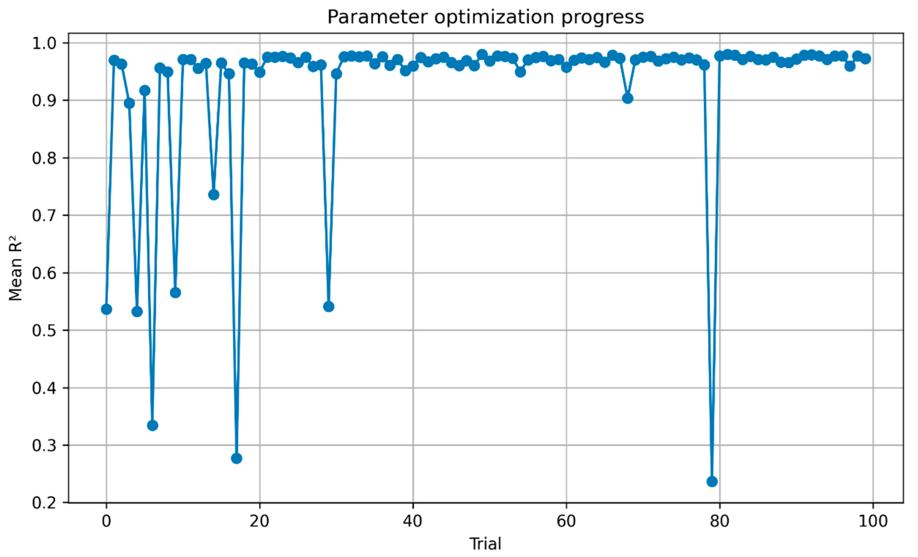
Figure 14 illustrates the optimization trajectory of the CNN–GRU model during hyperparameter tuning. The vertical axis represents the mean determination coefficient (R
2) across validation folds, while the horizontal axis corresponds to the number of optimization trials. At the early stage of the search, substantial fluctuations are observed, with R
2 values ranging from approximately 0.3 to 0.95, reflecting the sensitivity of model performance to different parameter combinations. As the optimization progresses, the search space becomes more effectively explored, and the performance rapidly stabilizes above R
2 = 0.9 after roughly 25 trials. Beyond this point, most candidate solutions remain consistently close to the optimal range, with only a few outliers indicating less effective configurations.
These results demonstrate the effectiveness of the optimization algorithm in identifying an appropriate CNN–GRU architecture and hyperparameters. By iteratively refining the search space, the algorithm avoids poor-performing configurations and converges towards a highly reliable solution. The final optimized model achieves an average R
2 above 0.95, confirming that the selected hyperparameters significantly enhance the predictive accuracy and robustness of dam deformation forecasting.
Table 1 and
Table 2 summarize the hyperparameter optimization process for the proposed CNN–GRU model. As shown in
Table 1, six key parameters were selected for optimization, including the number of convolutional filters, kernel size, GRU hidden size, dense layer units, dropout rate, and learning rate. The search space was defined to balance model flexibility with computational efficiency, covering both discrete sets (e.g., CNN filters, GRU hidden size, dense units) and continuous ranges (e.g., dropout rate, learning rate). The optimization results in
Table 2 indicate that the best-performing configuration consists of 64 CNN filters, a kernel size of 3, a GRU hidden size of 256, 128 dense units, a dropout rate of 0.2, and a learning rate of 1 × 10
−3. These values correspond to a compact yet expressive architecture that effectively captures spatiotemporal features while avoiding overfitting. In particular, the relatively small dropout rate (0.2) ensures regularization without sacrificing feature learning, and the optimized learning rate enables stable convergence during training.
4.2. Multi-Point Dam Deformation Predictive Performance Evaluation
Figure 15 shows the comparison of the dam displacement results using the constructed deep learning method and multiple linear regression. Across all subplots, the developed CNN-GRU predictions exhibit a closer alignment with the measured deformation values, effectively capturing both the seasonal variations and the short-term fluctuations. In contrast, the MLR predictions deviate substantially from the true values, especially during periods of rapid deformation changes, showing a persistent overestimation trend. These experimental results highlight two major advantages of the proposed method. First, by integrating convolutional layers with recurrent units, the CNN–GRU framework successfully extracts temporal dependencies and nonlinear relationships from the monitoring data, which are overlooked by the linear regression model. Second, the improved predictive accuracy across different locations demonstrates the robustness and generalizability of the proposed approach in handling heterogeneous dam response patterns. Taken together, the CNN–GRU model provides a more reliable tool for dam deformation forecasting, offering stronger potential for early warning and safety assessment than traditional regression-based methods.
Table 3 compares the predictive performance of the proposed CNN–GRU model with the conventional multiple linear regression (MLR) method across four monitoring points (TCN08, TCN09, TCN10, and TCN13). The CNN–GRU consistently achieves higher R2 values (0.7364–0.9222) than MLR, which shows limited explanatory power and even negative R2 at TCN13. Moreover, the CNN–GRU substantially reduces RMSE, MAE, and MAPE across most points, with improvements being particularly significant at TCN08, TCN09, and TCN13. These results indicate that the deep learning approach not only enhances overall prediction accuracy but also provides more stable and reliable estimates in complex deformation scenarios.
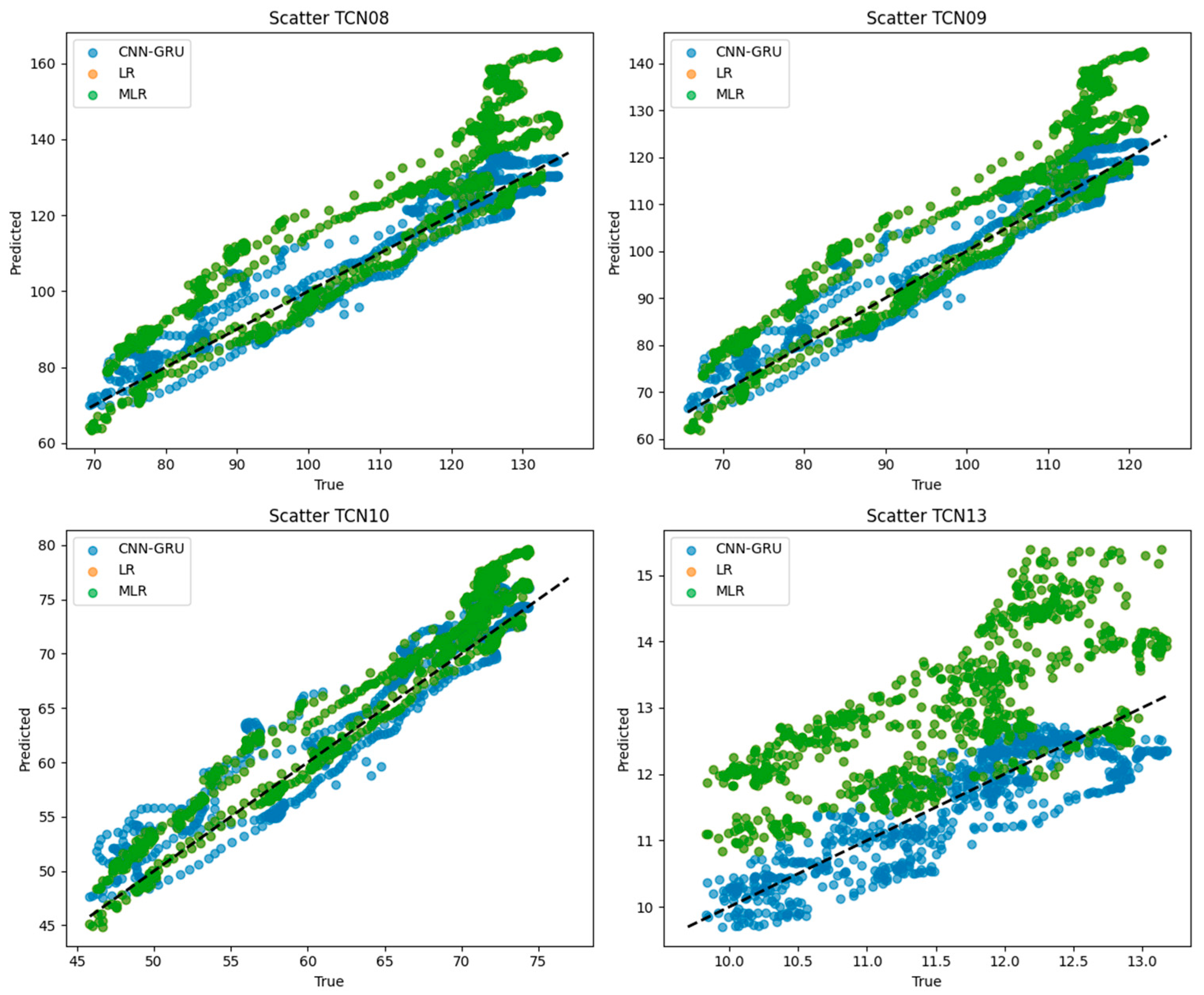
Figure 16 presents scatter plots of predicted versus observed dam deformation at four monitoring points (TCN08, TCN09, TCN10, and TCN13) using the proposed CNN–GRU model, linear regression (LR), and multiple linear regression (MLR). For CNN–GRU, the prediction points are more tightly clustered around the 1:1 reference line, indicating higher accuracy and lower bias across all locations. In contrast, MLR shows substantial deviations, especially at TCN08, TCN09, and TCN13, where systematic overestimation is evident. LR performs moderately but still exhibits larger dispersion compared with CNN–GRU. Overall, the figure highlights the superior predictive capability and robustness of the deep learning approach in capturing complex deformation behaviors compared to conventional regression methods.
4.3. Comparative Models
To validate the effectiveness of the proposed CNN-GRU-based deformation prediction framework, several comparative models were constructed and evaluated using the same dataset and experimental protocol. These models include both traditional statistical approaches and modern machine learning methods commonly used in time series forecasting:
Multiple Linear Regression (MLR): A baseline statistical model that assumes linear relationships among variables, serving as a reference for evaluating the added value of nonlinear modeling.
Support Vector Regression (SVR): A kernel-based learning method that captures limited nonlinearity in small- to medium-sized datasets. A radial basis function (RBF) kernel was employed with hyperparameters optimized via grid search.
Random Forest Regression (RFR): An ensemble-based model that handles nonlinearity and feature interactions by aggregating multiple decision trees. The number of estimators and tree depth were tuned for optimal performance.
Long Short-Term Memory (LSTM): A widely used recurrent neural network model for sequence modeling. The LSTM was configured with one to two hidden layers, and its architecture was optimized to match the input feature dimensionality.
Gated Recurrent Unit (GRU): A simplified variant of LSTM, used to isolate the effect of convolutional feature extraction by comparing it directly with the GRU component in the proposed CNN-GRU model.
All models were trained and evaluated using the same preprocessed dataset. Hyperparameters were tuned using randomized cross-validation or Bayesian optimization where applicable. Evaluation metrics included Root Mean Squared Error (RMSE), Mean Absolute Error (MAE), and Coefficient of Determination.
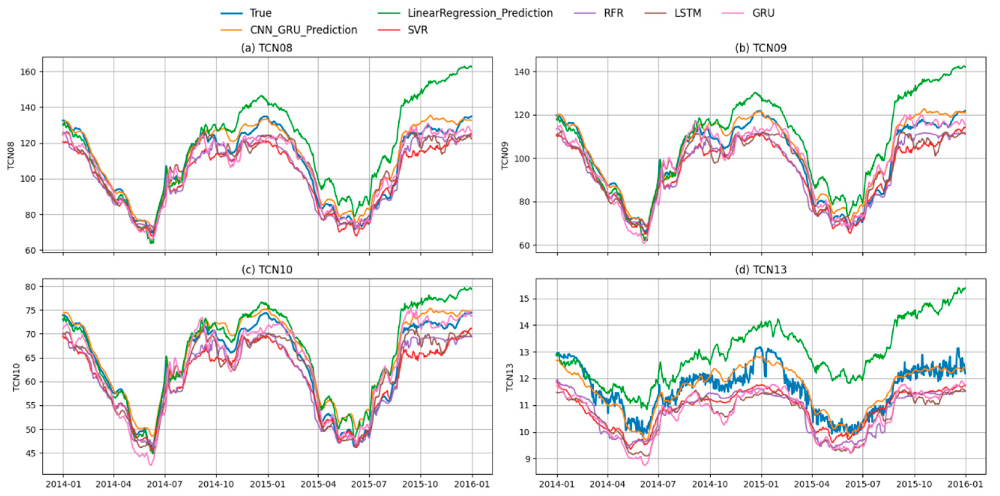
Figure 17 and
Figure 18 present the time-series prediction results and corresponding evaluation metrics of different models at four typical monitoring points (TCN08, TCN09, TCN10, and TCN13). The proposed CNN–GRU hybrid model consistently demonstrates superior predictive performance compared to traditional machine learning models (Linear Regression, SVR, RFR) and standalone deep learning architectures (LSTM and GRU). In
Figure 17, the CNN–GRU predictions closely follow the ground truth across all monitoring points, capturing both long-term deformation trends and short-term fluctuations. By contrast, Linear Regression deviates significantly, especially under nonlinear variations, and tends to over- or under-estimate deformation levels. SVR and RFR reduce part of this bias but still exhibit noticeable divergence during rapid deformation stages. LSTM and GRU show relatively good agreement with the measured data, but their predictions exhibit either smoother trajectories or small phase shifts that weaken the accuracy. The CNN–GRU model effectively balances these issues, showing both stability and responsiveness to deformation dynamics. In
Figure 18, the evaluation metrics (R
2, RMSE, MAE, and MAPE) further highlight the advantage of the CNN–GRU approach. At all monitoring points, CNN–GRU yields the highest R
2 values and the lowest error measures, reflecting its ability to generalize across different deformation regimes. Linear Regression shows the weakest performance, with very low R
2 and high errors, while SVR and RFR perform moderately. Deep learning baselines (LSTM and GRU) improve the prediction quality, yet CNN–GRU consistently outperforms them, indicating that combining CNN’s spatial feature extraction with GRU’s temporal modeling strengthens predictive capability.
This conclusion is further validated in
Table 4, where the CNN–GRU model achieves the best overall results with R
2 = 0.9582, RMSE = 4.1121, MAE = 3.1786, and MAPE = 3.1061. Compared to the next-best GRU model, CNN–GRU reduces RMSE by more than 20% and improves accuracy metrics across the board. Importantly, the CNN–GRU framework surpasses conventional methods by a large margin: compared to Linear Regression, the R
2 is nearly doubled, and the error metrics are reduced to less than one-third.
5. Conclusions and Future Work
This study proposes a CNN–GRU-based deep learning framework for long-sequence deformation prediction in hydropower stations. Compared with conventional regression models (e.g., Linear Regression, SVR, RFR) and single deep learning architectures (LSTM, GRU), the proposed method exhibits clear advantages. Qualitative analysis of time-series predictions demonstrates that CNN–GRU better captures both long-term deformation trends and short-term fluctuations, avoiding the systematic bias observed in traditional models and the over-smoothing effects seen in some deep learning baselines. Quantitative comparisons further confirm its superiority: the CNN–GRU model achieves the highest coefficient of determination (R2 = 0.9582) and the lowest error metrics (RMSE = 4.1121, MAE = 3.1786, MAPE = 3.1061), outperforming all competing approaches. These results highlight the model’s strong capability to extract spatial–temporal features from complex monitoring data and to generalize across different deformation regimes. Therefore, the proposed framework provides a more accurate and robust tool for real-time structural health monitoring and early risk assessment in hydropower station management. Future work will extend this approach by incorporating uncertainty quantification and online learning mechanisms to further improve adaptability under evolving environmental and operational conditions.
In addition, the ability of the proposed framework to generalize across different deformation regimes indicates its robustness in dealing with diverse hydrological and environmental conditions. This robustness is critical in real-world hydropower facility monitoring, where structural responses are influenced by a wide range of time-varying factors such as reservoir water levels, seasonal temperature variations, and material creep effects. By integrating convolutional layers for local feature extraction with GRUs for long-term sequence modeling, the framework provides a unified architecture capable of addressing both short- and long-term deformation dynamics.
While the CNN–GRU model shows strong predictive capability, several avenues remain for further advancement. First, incorporating uncertainty quantification into the modeling framework would provide probabilistic confidence bounds, enabling risk-informed decision-making in dam safety management. Second, developing online learning mechanisms could enhance adaptability by allowing the model to update its parameters in real time as new monitoring data become available, which is essential for capturing evolving nonstationary environmental influences.
Moreover, future studies should explore the integration of multimodal monitoring data, including temperature, reservoir water level, seepage, and vibration signals, to construct a more holistic representation of dam behavior. Such multimodal fusion would allow the model to disentangle overlapping influences and improve interpretability. Finally, addressing the challenge of model explainability remains a pressing research direction, especially in safety-critical domains such as hydropower facility monitoring. The incorporation of interpretable AI techniques could provide insights into the physical drivers of deformation, thereby enhancing stakeholder trust and facilitating practical deployment in real-world dam safety management systems.
In future work, we will further investigate the relative importance of the numerous input factors used for displacement prediction. Since deep learning models such as CNN–GRU are limited in directly providing interpretability, ensemble learning and model-agnostic interpretability techniques (e.g., Random Forests, Gradient Boosting, SHAP) will be introduced to quantify the contributions of different factors. This will allow us to identify the most influential variables, eliminate redundant inputs, and thereby enhance both the robustness and interpretability of dam deformation prediction models.
Author Contributions
Conceptualization, J.L. and C.G.; methodology, J.W. and Y.D.; investigation, J.L. and S.H.; writing—original draft preparation, J.L.; writing—review and editing, C.G., Y.D. and S.H.; project administration, C.G. and Y.D.; funding acquisition, J.L. All authors have read and agreed to the published version of the manuscript.
Funding
This research was funded by the National Key R&D Program Project (2023YFF0614303).
Data Availability Statement
Data used are available on request from the corresponding author. The data are not publicly available due to privacy.
Conflicts of Interest
Author Yongli Dong was employed by the company Zhengzhou Water Resources Construction Surveying and Design Institute Group Co., Ltd. The remaining authors declare that the research was conducted in the absence of any commercial or financial relationships that could be construed as a potential conflict of interest.
References
- Lu, X.; Chen, C.; Li, Z.; Chen, J.; Pei, L.; He, K. Bayesian Network Safety Risk Analysis for the Dam–Foundation System Using Monte Carlo Simulation. Appl. Soft Comput. 2022, 126, 109229. [Google Scholar] [CrossRef]
- Wang, S.; Xu, C.; Liu, Y.; Wu, B. Mixed-Coefficient Panel Model for Evaluating the Overall Deformation Behavior of High Arch Dams Using the Spatial Clustering. Struct. Control Health Monit. 2021, 28, e2809. [Google Scholar] [CrossRef]
- Yuan, D.; Gu, C.; Qin, X.; Shao, C.; He, J. Performance-Improved TSVR-Based DHM Model of Super High Arch Dams Using Measured Air Temperature. Eng. Struct. 2022, 250, 113400. [Google Scholar] [CrossRef]
- Zheng, S.; Shao, C.; Gu, C.; Xu, Y. An Automatic Data Process Line Identification Method for Dam Safety Monitoring Data Outlier Detection. Struct. Control Health Monit. 2022, 29, e2948. [Google Scholar] [CrossRef]
- Chen, X.; Chen, Z.; Hu, S.; Gu, C.; Guo, J.; Qin, X. A Feature Decomposition-Based Deep Transfer Learning Framework for Concrete Dam Deformation Prediction with Observational Insufficiency. Adv. Eng. Inform. 2023, 58, 102175. [Google Scholar] [CrossRef]
- Li, Y.; Zhao, H.; Gu, H.; Wei, Y.; Xiang, Z.; Wang, Y.; Yu, Y.; Bao, T. Automated Defect Segmentation and Quantification in Concrete Structures via Unmanned Aerial Vehicle-based Lightweight Deep Learning. Comput.-Aided Civ. Eng. 2025, mice.70062. [Google Scholar] [CrossRef]
- Wu, Z.; Li, J.; Gu, C.; Su, H. Review on Hidden Trouble Detection and Health Diagnosis of Hydraulic Concrete Structures. Sci. China Ser. E Technol. Sci. 2007, 50, 34–50. [Google Scholar] [CrossRef]
- Chen, B.; Wu, Z.; Liang, J.; Dou, Y. Time-Varying Identification Model for Crack Monitoring Data from Concrete Dams Based on Support Vector Regression and the Bayesian Framework. Math. Probl. Eng. 2017, 2017, 5450297. [Google Scholar] [CrossRef]
- Shu, X.; Bao, T.; Li, Y.; Gong, J.; Zhang, K. VAE-TALSTM: A Temporal Attention and Variational Autoencoder-Based Long Short-Term Memory Framework for Dam Displacement Prediction. Eng. Comput. 2022, 38, 3497–3512. [Google Scholar] [CrossRef]
- Yao, K.; Wen, Z.; Yang, L.; Chen, J.; Hou, H.; Su, H. A Multipoint Prediction Model for Nonlinear Displacement of Concrete Dam. Comput.-Aided Civ. Infrastruct. Eng. 2022, 37, 1932–1952. [Google Scholar] [CrossRef]
- Jia, D.; Yang, J.; Ma, C.; Cheng, L.; Xiao, S.; Gong, X. Research on Arch Dam Deformation Prediction Method Based on Interpretability Clustering and Panel Data Model. Eng. Struct. 2025, 329, 119794. [Google Scholar] [CrossRef]
- Xu, B.; Zhang, H.; Gu, C.; Chen, Z.; Gu, H. Multi-Target Prediction and Dynamic Interpretation Method for Displacement of Arch Dam with Cracks Based on a-DSRSN and SHAP. Adv. Eng. Inform. 2025, 66, 103467. [Google Scholar] [CrossRef]
- Cao, W.; Wen, Z.; Su, H. Spatiotemporal Clustering Analysis and Zonal Prediction Model for Deformation Behavior of Super-High Arch Dams. Expert Syst. Appl. 2023, 216, 119439. [Google Scholar] [CrossRef]
- Tian, J.; Chen, C.; Lu, X.; Li, Y.; Chen, J. Deep Transfer Learning-Based Time-Varying Model for Deformation Monitoring of High Earth-Rock Dams. Eng. Appl. Artif. Intell. 2024, 138, 109310. [Google Scholar] [CrossRef]
- Bian, K.; Wu, Z. Data-Based Model with EMD and a New Model Selection Criterion for Dam Health Monitoring. Eng. Struct. 2022, 260, 114171. [Google Scholar] [CrossRef]
- Wu, Y.; Kang, F.; Zhu, S.; Li, J. Data-Driven Deformation Prediction Model for Super High Arch Dams Based on a Hybrid Deep Learning Approach and Feature Selection. Eng. Struct. 2025, 325, 119483. [Google Scholar] [CrossRef]
- Bowen, W.; Zhaoxing, L.; Dongyang, Y. Optimized Deformation Monitoring Models of Concrete Dam Considering the Uncertainty of Upstream and Downstream Surface Temperatures. Eng. Struct. 2023, 288, 115950. [Google Scholar] [CrossRef]
- Li, M.; Ren, Q.; Li, M.; Fang, X.; Xiao, L.; Li, H. A Separate Modeling Approach to Noisy Displacement Prediction of Concrete Dams via Improved Deep Learning with Frequency Division. Adv. Eng. Inf 2024, 60, 102367. [Google Scholar] [CrossRef]
- Alhebrawi, M.N.; Huang, H.; Wu, Z. Artificial Intelligence Enhanced Automatic Identification for Concrete Cracks Using Acoustic Impact Hammer Testing. J. Civ. Struct. Health Monit. 2022, 13, 469–484. [Google Scholar] [CrossRef]
- Plehiers, P.P.; Symoens, S.H.; Amghizar, I.; Marin, G.B.; Stevens, C.V.; Van Geem, K.M. Artificial Intelligence in Steam Cracking Modeling: A Deep Learning Algorithm for Detailed Effluent Prediction. Engineering 2019, 5, 1027–1040. [Google Scholar] [CrossRef]
- Zhong, W.; Li, Y.; Zhang, Y.; Zhou, T.; Li, K.; Yang, T. A Dual-Branch Spatiotemporal Feature Fusion Prediction Model for Concrete Arch Dam Deformation Based on Multi-Scale Hierarchical Clustering. Adv. Eng. Inform. 2025, 68, 103782. [Google Scholar] [CrossRef]
- Wu, B.; Niu, J.; Deng, Z.; Li, S.; Jiang, X.; Qian, W.; Wang, Z. A Multiple-point Deformation Monitoring Model for Ultrahigh Arch Dams Using Temperature Lag and Optimized Gaussian Process Regression. Struct. Control Health Monit. 2024, 2024, 2308876. [Google Scholar] [CrossRef]
- Gu, H.; Li, Y.; Fang, Y.; Wang, Y.; Yu, Y.; Wei, Y.; Xu, L.; Chen, Y. Environmental-aware Deformation Prediction of Water-related Concrete Structures Using Deep Learning. Comput.-Aided Civ. Infrastruct. Eng. 2025, 40, 2130–2151. [Google Scholar] [CrossRef]
- Gopalakrishnan, K.; Khaitan, S.K.; Choudhary, A.; Agrawal, A. Deep Convolutional Neural Networks with Transfer Learning for Computer Vision-Based Data-Driven Pavement Distress Detection. Constr. Build. Mater. 2017, 157, 322–330. [Google Scholar] [CrossRef]
- Zhu, Y.; Xie, M.; Zhang, K.; Li, Z. A Dam Deformation Residual Correction Method for High Arch Dams Using Phase Space Reconstruction and an Optimized Long Short-Term Memory Network. Mathematics 2023, 11, 2010. [Google Scholar] [CrossRef]
- Li, M.; Ren, Q.; Li, M.; Qi, Z.; Tan, D.; Wang, H. Multivariate Probabilistic Prediction of Dam Displacement Behaviour Using Extended Seq2Seq Learning and Adaptive Kernel Density Estimation. Adv. Eng. Inform. 2025, 65, 103343. [Google Scholar] [CrossRef]
- Dey, R.; Salem, F.M. Gate-Variants of Gated Recurrent Unit (GRU) Neural Networks. In Proceedings of the 2017 IEEE 60th international midwest symposium on circuits and systems (MWSCAS), Boston, MA, USA, 6–9 August 2017; pp. 1597–1600. [Google Scholar]
Figure 1.
Schematic diagram of a convolutional neural network.
Figure 1.
Schematic diagram of a convolutional neural network.
Figure 2.
Diagram of the GRU network.
Figure 2.
Diagram of the GRU network.
Figure 3.
Diagram of the CNN-multi-stacked-GRU network.
Figure 3.
Diagram of the CNN-multi-stacked-GRU network.
Figure 4.
Schematic diagram of the improved PSO algorithm.
Figure 4.
Schematic diagram of the improved PSO algorithm.
Figure 5.
Parameter optimization process.
Figure 5.
Parameter optimization process.
Figure 6.
The overall layout of the project.
Figure 6.
The overall layout of the project.
Figure 7.
Dam deformation safety monitoring system.
Figure 7.
Dam deformation safety monitoring system.
Figure 8.
Long-term monitoring data and statistical characterization of hydraulic variables.
Figure 8.
Long-term monitoring data and statistical characterization of hydraulic variables.
Figure 9.
Visualization of long sequence measured data of the thermometer sensor.
Figure 9.
Visualization of long sequence measured data of the thermometer sensor.
Figure 10.
Correlation analysis of thermometer sensor data.
Figure 10.
Correlation analysis of thermometer sensor data.
Figure 11.
Visualization results of the dam displacement monitoring data.
Figure 11.
Visualization results of the dam displacement monitoring data.
Figure 12.
Statistical distributions of displacement measurements.
Figure 12.
Statistical distributions of displacement measurements.
Figure 13.
The process line of the model training process changes with the number of iterations.
Figure 13.
The process line of the model training process changes with the number of iterations.
Figure 14.
Evaluation index change process line of deep neural network hyperparameter optimization process.
Figure 14.
Evaluation index change process line of deep neural network hyperparameter optimization process.
Figure 15.
Evaluation and comparison of the developed DL-based dam deformation model and statistical model.
Figure 15.
Evaluation and comparison of the developed DL-based dam deformation model and statistical model.
Figure 16.
Predicted versus observed dam deformation at different monitoring points.
Figure 16.
Predicted versus observed dam deformation at different monitoring points.
Figure 17.
Comparative evaluation of multiple displacement prediction methods.
Figure 17.
Comparative evaluation of multiple displacement prediction methods.
Figure 18.
Visual analysis of monitoring data.
Figure 18.
Visual analysis of monitoring data.
Table 1.
Deep learning models require parameter optimization.
Table 1.
Deep learning models require parameter optimization.
| Parameter | Search Space |
|---|
| CNN filters | {32, 64, 96, 128} |
| Kernel size | [2, 5] (integer) |
| GRU hidden size | {64, 128, 192, 256} |
| Dense units | {128, 192, 256, 320, 384, 448, 512} |
| Dropout rate | [0.2, 0.5] (continuous uniform) |
| Learning rate | [1 × 10⁻⁵, 1 × 10⁻²] (log-uniform) |
Table 2.
Deep learning parameter optimization results.
Table 2.
Deep learning parameter optimization results.
| Parameter | Optimal Value |
|---|
| CNN filters | 64 |
| Kernel size | 3 |
| GRU hidden size | 256 |
| Dense units | 128 |
| Dropout rate | 0.2 |
| Learning rate | 1 × 10⁻³ |
Table 3.
Comparison of prediction results between deep learning and statistical regression methods.
Table 3.
Comparison of prediction results between deep learning and statistical regression methods.
| Monitoring Point | | CNN_GRU | | | | | MLR | |
|---|
| | R2 | RMSE | MAE | MAPE | R2 | RMSE | MAE | MAPE |
|---|
| TCN08 | 0.9222 | 5.6095 | 4.6634 | 4.5075 | 0.4889 | 14.3748 | 0.4889 | 14.3748 |
| TCN09 | 0.9106 | 5.1448 | 4.2415 | 4.4676 | 0.6095 | 10.7546 | 0.6095 | 10.7546 |
| TCN10 | 0.8821 | 3.0552 | 2.5658 | 4.2212 | 0.8739 | 3.1588 | 0.8739 | 3.1588 |
| TCN13 | 0.7364 | 0.4526 | 0.3725 | 3.1754 | −2.1193 | 1.5571 | −2.1193 | 1.5571 |
Table 4.
Comparison of the results of different deformation prediction methods.
Table 4.
Comparison of the results of different deformation prediction methods.
| Models | R2 | RMSE | MAE | MAPE |
|---|
| CNN_GRU_Prediction | 0.9582 | 4.1121 | 3.1786 | 3.1061 |
| LinearRegression_Prediction | 0.4889 | 14.3748 | 11.5837 | 10.6624 |
| SVR | 0.8442 | 7.9357 | 6.9990 | 6.1888 |
| RFR | 0.8901 | 6.6659 | 5.9336 | 5.3422 |
| LSTM | 0.9114 | 5.9870 | 4.9716 | 4.5634 |
| GRU | 0.9339 | 5.1688 | 4.0768 | 3.8109 |
| Disclaimer/Publisher’s Note: The statements, opinions and data contained in all publications are solely those of the individual author(s) and contributor(s) and not of MDPI and/or the editor(s). MDPI and/or the editor(s) disclaim responsibility for any injury to people or property resulting from any ideas, methods, instructions or products referred to in the content. |
© 2025 by the authors. Licensee MDPI, Basel, Switzerland. This article is an open access article distributed under the terms and conditions of the Creative Commons Attribution (CC BY) license (https://creativecommons.org/licenses/by/4.0/).

