Phosphorus Retention in Treatment Wetlands? A Field Experiment Approach: Part 1, Hydrology

Abstract

Stormwater Treatment Areas (STAs) are large wetlands constructed to reduce phosphorus (P) from agricultural and urban runoff into the Everglades Protection area. Wetland vegetation in these STAs reduce P in surface water, affects flow resistance, and causes delays of water deliveries. Vegetation resistance is commonly determined by the flow regime and vegetation porosity. Field experiments were conducted to seek alternative ways to estimate vegetation resistance in STAs. We generated small sinusoidal discharge perturbations superimposed on near-steady state flow conditions and measured in situ water levels inside the wetland. The elapsed time for the generated waves to reach various locations and wave amplitude attenuations inside the wetland were used to calculate porosity/transmissivity (K), a single parameter representing vegetation resistance. The vegetation index combined with calculated K distribution indicated that transmissivity is a straightforward way to represent vegetation resistance. High K values indicate sparse vegetation density or open water (low vegetation index), resulting in low vegetation resistance. Low K values indicate high vegetation density (high vegetation index), resulting in high vegetation resistance independent of vegetation and flow type. This manuscript describes a field experiment and discusses the relationship between K and the vegetation index (representing vegetation density). Part II will present the consequences of water movement on P retention in these systems.

1. Introduction

The Florida Everglades is a subtropical wetland that once encompassed 1.2 × 10⁴ km² of Southern Florida and extended 160 km from south of Lake Okeechobee to the mangrove estuaries of Florida Bay and the Gulf of Mexico. At half of its original extent, the remaining system is contained within the boundaries of the Water Conservation Areas (WCAs) and the Everglades National Park (ENP). Historically, the Everglades was an oligotrophic peatland system that received its water and nutrients via rainfall [1]. Much of the Everglades north and west of the WCAs has been converted to farmland, locally known as the Everglades Agricultural Area (EAA), which is a major source of water that flows into the Water Conservation Areas (WCAs), and the Everglades National Park (ENP). Human control of system hydrology facilitated the draining of half of the original Everglades for agricultural and urban use, resulting not only in the loss of habitat but also in water quality changes, particularly phosphorus (P). The introduction of excessive P to the oligotrophic Florida Everglades system caused shifts in the floral and faunal communities [2,3]. Surface water concentrations of total phosphorus (TP) in the Everglades are typically less than 10 μg·L⁻¹. Historically, the principal external source of phosphorus to the marsh was rainfall [4].

The South Florida Water Management District (SFWMD) is implementing the Restoration Strategies (RS) Program (https://www.sfwmd.gov/our-work/restoration-strategies, accessed on 15 May 2024) that has created more than 6500 acres of Stormwater Treatment Areas (STAs) and 110,000 acre-feet of additional water storage through construction of Flow Equalization Basins (FEBs) to achieve the mandated water-quality-based effluent limit (WQBEL) to correct this problem and is described in State of Florida and FDEP (2017) as follows: Shall not exceed 13 as an annual flow-weighted mean (FWM) in more than 3 out of 5 water years on a rolling basis and 19 ppb as an annual flow-weighted mean (AFWM) in any water year, where ppb is part per billion (equivalent to µg·L⁻¹; https://floridadep.gov/ecopro/eco-pro/content/everglades-forever-act, accessed on 12 April 2022).

FEBs serve two main functions: they alleviate peak flow during the wet season and provide water to supply the STAs during the dry season to prevent soil dry outs (P oxidation and P release upon re-wetting of soil). Those STAs and FEBs contain emergent aquatic vegetation (EAV), submerged aquatic vegetation (SAV), and areas of open water.

The management of STAs and FEBs is an emerging science. The optimal design and operation of these features require a detailed understanding of the vegetation dynamics within the STA and an understanding of the hydraulics and timing associated with maintaining healthy vegetation in those systems. The objective of this field experiment is to understand if the combined interaction between vegetation representation in STAs (e.g., vegetation density or a surrogate of vegetation density) and hydraulic behavior, due to vegetation resistance, can be expressed by a single (bulk) parameter.

The earliest attempts to understand vegetation resistance depended on developing analytical expressions. The initial analytical efforts were based on rigid cylindrical bodies to represent vegetation. The authors of [5] were among the first who developed an equation relating drag coefficient to flow velocity and other parameters. In [6], innovative ideas were introduced that included flexible stems into equations for vegetation resistance. Reynolds averaging and turbulent flow equations were used by [7] after considering vegetation as a porous media. Laboratory plumes were used to determine and verify vegetation resistance by [8] and many others. Equations describing vegetation resistance developed during this time were used with Manning’s equation when designing vegetated flow ways.

In the South Florida wetlands, Lee et al. (2004) [9] experimented with sawgrass in a flume to determine formulas for roughness in terms of drag coefficients. They determined that the Manning’s equation is not appropriate to represent vegetation resistance in wetlands. The authors of [10] used field experiments in constructed wetlands, along with laboratory and numerical methods, to determine resistance caused by emergent vegetation. Results for most of the previous studies were presented in terms of Manning’s equation, the Darcy–Weisbach friction factor, or the drag coefficient of plant stems. On the other hand, Kadlec and Wallace (2009) [11] used a general power law equation to describe friction losses in flow due to vegetation. They pointed out the importance of site-specific factors and showed that some generalized parameters cannot be easily extrapolated to other locations due to the influence of several factors such as vegetation type, vegetation density, and season of the year. Unknown factors such as topographic variability, drainage canals, and organic accretion of dead vegetation also influence vegetation resistance. Yet [12,13] provided innovative approaches to estimate vegetation resistance as a function of flow discharge and in terms of bulk vegetation porosity, respectively. Contour maps of bulk vegetation porosity in terms of discharge flow in two STAs were also presented [14].

Recently, Lal et al., (2015) [13,14] described in detail a field experiment that estimated vegetation resistance in a large, constructed wetland. Similar to [11], they recommended a power function be used instead of Manning’s n to estimate vegetation resistance. Their analysis specified three different power law functions representing three different flow types in the same STA and concluded the need for a single formula or parameter to represent vegetation resistance for all wetland flow types. This single parameter should be obtained directly from field observations to describe vegetation resistance. The primary goal of this study is to confirm and build on the previous field test studies of [13,14] and explore the potential to develop a single bulk parameter to represent vegetation resistance. Primarily, that single parameter is calculated directly from field observations, independent of vegetation and flow type. This single vegetation resistance parameter should also provide clues on how water moves inside a large, constructed wetland to identify short circuiting and enhance P retention.

2. Materials and Methods

Two field experiments were conducted in STA-3/4 and STA-2 (Figure 1), Palm Beach County, Florda USA. The field experiments described here were designed to investigate connections and relationships between water levels, inflow discharges, P-concentrations, and wetland vegetation properties. These field experiments were conducted in an EAV-dominated STA-3/4 Cell 2A (STA34C2A) and SAV dominated with areas of EAV STA-2 Cell 3 (STA2C3, Figure 1). The research focused on the EAV-dominated STA34C2A compared to a mixture of both EAV and SAV in STA2C3. The choice of those two locations to conduct the experiment was based on the aspect ratio of a wetland; the aspect ratio is a numerical representation that describes the proportional relationship between the width and the length of a rectangular shape. Both STAs differed greatly in their aspect ratio (0.43 vs. 0.78 for STA2C3 and STA34C2A, respectively), almost twice as much, and certainly STA2C3 was much longer (4600 m [m] vs. 3600 m) compared to STA34C2A (Figure 1C,D). The construction of those large STAs is very costly. For example, building a flow way comprising several small-aspect ratio treatments is cost prohibitive and far more expensive compared to constructing an exceptionally long flow way with an aspect ratio similar to STA2C3. The phosphorus effect due to the aspect ratio of a treatment cell will be the focus of Part II.

Small sinusoidal discharges were generated on top of near-steady-state flow conditions. Wave speed and attenuation characteristics at various locations within the wetland were measured. These characteristics were used to explore vegetation resistance parameters and provided estimates of vegetation resistance. Wave speed and wave amplitude attenuations were used to determine the time of wave arrivals at specific water level loggers, which provided the basis to estimate bulk vegetation resistance and transmissivity.

2.1. Experiment Location

This field experiment was conducted in (STA34C2A, 26°22′40″ and −80°37′16″), which was heavily vegetated, with dense strands of cattail (Typha sp.; Figure 2A) at the time of the experiment. STA34C2A was the focus for the hydraulic field experiment because it is dominated by a single vegetation type (EAV). On the contrary, STA2C3 is a mixture of SAV, EAV, and open water. Many STAs, including the study site, have remnant agricultural canals in the traverse direction of flow. Most of the transverse canals are perpendicular to the southerly flow and some have small remnant levees that affect water flow (Figure 2A). Data collected from STA34C2A were used to (1) investigate the wetland’s hydraulics, (2) ratify results obtained from an EAV-dominated wetland study in STA34C3A [13], and (3) explore other potential approaches to determine vegetation resistance in terms of vegetation density. Water quality (phosphorus) data analyses and modeling results will be presented in Part 2 of this research.

2.2. Hydraulic Monitoring

The most important aspect of the field experiment was to control the inflow discharges remotely and create very distinct signals in the system that were easy to identify and to use when calculating or characterizing parameters, using analytical solutions and inverse engineering methods. The field test was conducted by generating small sinusoidal discharge perturbations (waves) superimposed on near-steady-state conditions. Sinusoidal waves of a single unique frequency were selected with each test to isolate the influence of the test disturbance from many other water level disturbances present in the system such as daily and half-daily cycles. During the test, wave speed and attenuation characteristics at different stations of the wetland were measured.

The STA-3/4 hydraulic field experiment took place between 8 August 2014 and 24 September 2014, during which high- and low-frequency waves were sent through the G377 structures (Figure 2B). Portable water level loggers (Solinst Leveloggers Edge 3001, Solinst Canada LTD, Georgetown, ON, Canada) were deployed to measure changes in water surface elevation every 15 min. The locations of those loggers were set at equal distance, as practically as possible (i.e., 701–841 m), from each other and placed in a grid (Figure 2B). Helicopter flights were used to deploy the loggers. One Solinst Baro-logger was deployed to measure atmospheric pressure at the field experiment site (St #44 on the eastern side of Cell 2A; Figure 2B), which was subtracted from water level loggers’ measurements to only obtain water pressure at all station locations within the wetland.

At the conclusion of sending all the waves for a field test, and prior to retrieving the data loggers from the field test site, one must perform a “ponding” test, which is a flat-pool test. This ponding technique (no inflow and outflow for at least 2–3 days), ensures that those portable water level loggers’ readings can be related to fixed and surveyed permanent-stage recorders such as G377T and G378H (Figure 2B). Tail and head water readings from the inflow and outflow structures at the ponding time (i.e., 15 August 2014 06:00; Figure 3) are then used to introduce the adjustment needed for every deployed sensor. Head and tail water readings are “stage,” which is related to the vertical datum, NGVD 29. The adjustment, generated from the flat pool date and time stage reading, is then applied to all portable water level loggers’ readings.

2.3. Wave Generation

Field tests in South Florida using generated sinusoidal disturbances have previously been performed [13]. One of the goals of this field test was to send a distinct frequency unique to the region through the vegetation and analyze just that signal without any other disturbances. We avoided known frequencies such as half-daily and daily cycles (12 or 24 h). Waves with such periods may become confused by half-daily and daily cycles that are related to weather or daily operations through the control room. Instead, we selected odd frequencies to ensure that the selected wave period was distinguishable from other noises. In the case of this field test, the wave frequencies selected had periods of 64, 64, and 50 h.

Upstream discharges (through manipulation of culvert gates) at the inflow were used to generate disturbances in the vegetated medium, and downstream structures were fully open for flow. The total inflow discharge (Q) at the upstream end took the following form:

$$Q=Q_0+q_0\sin \left({\displaystyle \frac{2\pi t}{P}}\right)$$

(1)

where Q is the maximum flow available from the inflow structure used to create an equilibrium inflow rate; Q₀ is the average flow for this wave; q₀ = amplitude of the superimposed sinusoidal disturbance; P = wave period; and t = time. The value of Q₀ was selected to cover a wide range of water depths that exist in the STAs and not to exceed the maximum inflow structure capacity. A value of q₀ ranging between 0.2Q₀ and 0.5Q₀ was used to make sure that the discharge signal was not too large, so that the solution was in the non-linear range, and not too small so as to be undetectable at the outflow or last station location. A recommended guideline is that the amplitude ratio (amplitude at the last location site normalized by the amplitude at the inflow) should not be less than 0.20.

2.4. Governing Equation (Vegetation Resistance Equation)

The following power-law-type function for discharge per unit width q(h, s_f) describes the effect of flow resistance on discharge:

$$q(h,s_f)={\displaystyle \frac{1}{n_b}}{h}^{1+\gamma }|s_f{|}^{\alpha }\mathrm{sgn}(s_f)$$

(2)

where h = water depth, and s_f = friction slope or the slope of the energy grade line; sgn (s_f) = ±1 depending on s_f > 0 or s_f < 0; and where the preceding parameters n_b, α, and γ determine the static and dynamic character of the flow. The diffusion wave approximation of St. Venant’s equations can be linearized for small disturbance analysis in hydraulics. The power-law-type equation is differentiable to attain a simple expression for hydraulic diffusivity and wave speed.

$${\displaystyle \frac{\partial h}{\partial t}}+a(h,s_f){\displaystyle \frac{\partial h}{\partial x}}=K(h,s_f){\displaystyle \frac{{\partial }^{2}h}{\partial x^2}}$$

(3)

where a and K are defined as

$$a=\partial x{\displaystyle \frac{\partial h}{\partial t}}=(1+\gamma ){\displaystyle \frac{1}{n_b}}{h}_n^{\gamma }|S_{\mathit{fn}}{|}^{\alpha }\mathrm{sgn}(S_{fn})=(1+\gamma ){\displaystyle \frac{q_n}{h_n}}$$

(4)

$$K={\displaystyle \frac{\partial q}{\partial S_f}}=\alpha {\displaystyle \frac{1}{n_b}}{h}_n^{1+\gamma }|S_{\mathit{fn}}{|}^{\alpha -1}=\alpha {\displaystyle \frac{q_n}{S_{fn}}}$$

(5)

where a is the kinematic celerity [13], and K is the hydraulic diffusivity/transmissivity, a function of vegetation porosity (e.g., type, size, leaf, stem flexibility, density, etc.).

Wave parameters were then used to solve the inverse problem to calculate the vegetation resistance parameters. This involved calculating K and a using k₁ and k₂ values, which were calculated directly from field observations, and then using the following equations to solve the inverse problem [13]:

$$c={\displaystyle \frac{\Delta l}{\Delta t}}$$

(6)

where C is the wave speed, and ∆l and ∆t are the phase lag and the time of travel between the two-gauge locations, respectively.

$$k_1={\displaystyle \frac{1}{\Delta l}}\ln \left({\displaystyle \frac{y_{dn}}{y_{up}}}\right)$$

(7)

where k₂ is the wave number, f₂ is the wave frequency, and the decay coefficient k₁ is calculated using

$$k_2={\displaystyle \frac{f_{2}t}{\Delta l}}={\displaystyle \frac{f_2}{c}}$$

(8)

where y_up and y_dn are the amplitudes of the water wave observed at an upstream and a downstream gauge separated by a distance (∆l). Given k₁, k₂ and f₂, K and a are calculated as follows [13]:

$$K={\displaystyle \frac{f_2}{k_2}}{\displaystyle \frac{k_1}{\left(k_2^2+k_1^2\right)}}$$

(9)

$$a={\displaystyle \frac{f_2}{k_2}}{\displaystyle \frac{\left(k_2^2-k_1^2\right)}{\left(k_2^2+k_1^2\right)}}$$

(10)

where a = kinematic wave celerity/speed; K = hydraulic diffusivity, or transmissivity as applied to porous media flow (groundwater), if vegetation takes a negligible space. Once the K and a values are known, resistance parameters, (i.e., γ, α, and n_b) are calculated following [13] and are valid only for the range of parameters (Q, h, water slope) used in these tests. We used Equations (9) and (10) to calculate K (

Table A1. Transmissivity (K) values calculated from field observations in STA34C2A for all waves. It should be noted that the “S” station location is half-way between up-(y_up) and down-stream (y_dn) stations (e.g., St04 and St03), where the water level loggers are located.

Station	Longitude (West)	Latitude (North)	K (m2·s−1): Wave 1	K (m2·s−1): Wave 2	K (m2·s−1): Wave 3
S1	80°38′10.01″	26°23′33.89″	3.21	4.51	4.63
S2	80°37′48.84″	26°23′33.89″	3.13	3.88	5.54
S3	80°37′29.93″	26°23′33.89″	3.86	5.24	5.15
S4	80°37′13.26″	26°23′33.89″	Missing
S5	80°36′47.22″	26°23′33.89″	4.03	5.41	5.18
S6	80°38′9.65″	26°23′9.95″	21.49	8.82	20.89
S7	80°37′48.32″	26°23′9.95″	23.55	10.52	22.24
S8	80°37′22.17″	26°23′9.95″	10.43	15.65	29.49
S9	80°36′59.35″	26°23′9.95″	416.87	103.37	106.26
S10	80°36′37.33″	26°23′9.95″	19.44	9.16	17.31
S11	80°38′9.56″	26°22′47.87″	46.87	12.33	23.82
S12	80°37′45.14″	26°22′47.87″	95.07	21.73	27.52
S13	80°37′17.74″	26°22′47.87″	10.43	15.65	29.49
S14	80°36′53.09″	26°22′47.87″	416.87	103.37	106.26
S15	80°36′28.40″	26°22′47.87″	103.92	26.62	4.74
S16	80°38′9.62″	26°22′26.12″	100.7	168.87	15.83
S17	80°37′41.46″	26°22′26.12″	47.53	31.95	14.57
S18	80°37′11.31″	26°22′26.12″	60.83	11.83	16.35
S19	80°36′42.02″	26°22′26.12″	84.27	65.29	46.59
S20	80°36′19.95″	26°22′26.12″	139.53	283.54	25.48
S21	80°38′9.46″	26°22′0.05″	30.87	20.41	91.47
S22	80°37′37.57″	26°22′0.05″	38.42	26.88	98.15
S23	80°37′11.31″	26°22′0.05″	63.45	44.69	54.17
S24	80°36′31.74″	26°22′0.05″	36.11	20.72	35.45
S25	80°36′11.30″	26°22′0.05″	29.8	19.05	70.13

) and the a parameter.

2.5. Amplitudes, Phase Lags, and Wave Attenuation

Amplitudes and phase lags were calculated for all three wave trains using deployed water level data observed in the field (i.e., equation fitting;

Table A2. Summary results of wave/signal extraction. Amplitudes and phase lags of Wave 1 Period = 64 h and average discharge Q₀ = 21.23 m³·s⁻¹ (750 cfs ± 50%) inside STA34C2A.

Station # ID	Bias (a1) 2	Slope (a2) 3	Absolute Amplitude (a3) 4	Phase Lag (a4) 5 (hours)	∆t (hours)
St 32_0488	3.69845	−0.00015	0.03984	63.529	16.7738
St 22_0504	3.74202	−0.00031	0.03884	127.681	16.9258
St 21_0508	3.65123	−0.00025	0.0324	67.8628	21.1076
St 41_0511	3.66422	−0.00005	0.03218	131.219	20.4638
St 13_0515	3.75517	−0.00016	0.04777	124.513	13.7578
St 03_5020	3.76957	−0.00015	0.04733	60.405	13.6498
St 14_2829	3.8317	3.8317	0.0592	55.8663	9.1111
St 33_2850	3.7465	−0.00006	0.04384	125.276	14.5208
St 12_3951	3.72678	−0.00016	0.04097	−0.90803	16.33677
St 01_5439	3.6843	−0.0002	0.03433	130.422	19.6668
St 42_5899	3.70842	−0.0002	0.03816	129.001	18.2458
St 11_5904	3.67373	−0.00021	0.03447	2.76541	20.01021
St 24_5905	3.82075	−0.00011	0.0559	120.166	9.4108
St 02_6042	3.7266	−0.00017	0.03967	63.9225	17.1673
St 04_6754	3.83434	−0.00012	0.06	55.4888	8.7336
St 31_6757	3.67894	−0.00023	0.03472	66.5423	19.7871
St 43_8267	3.74289	−0.00024	0.04359	62.4727	15.7175
St 44_3939	3.79852	−0.00012	0.0512	121.67	10.9148
Q_G377	21.3526	−0.00151	10.6713	46.7552	0.000001 1
G377Tail	3.87634	−0.00011	0.0684	52.2403	5.4851
G378Head	3.54446	−0.00029	0.03095	70.0615	23.3063

Note: ¹ = starting time for ∆T at inflow site. ² = bias (a₁). ³ = slope (a₂). ⁴ = absolute value of the amplitude (a₃). ⁵ = phase lag in hours (a₄). Gray row represents values at inflow structure.

). Phase lags (i.e., arrival times) of the generated wave were calculated as the phase difference between the discharge wave at the inflow and the water level observed at each location (

Table A3. Wave amplitudes and phase lag results (for all three waves) obtained from the field experiment conducted in STA3/4 Cell 2A. Wave 1 period = 64 h and average discharge Q₀ = 21.24 m³·s⁻¹ (750 cfs ± 50%); Wave 2 period = 64 h and average discharge Q₀ = 9.91 m³·s⁻¹ (350 cfs ± 43%); Wave 3 period = 50 h and average discharge Q₀ = 25.49 m³·s⁻¹ (900 cfs ± 40%). Wave amplitudes at every logger location were normalized by the wave amplitude value at the inflow structure, which resulted in a normalized value of 1 at the G377.

	Wave 1		Wave 2		Wave 3
Station	Amplitude Ratio	Phase Lag (h)	Amplitude Ratio	Phase Lag (h)	Amplitude Ratio	Phase Lag (h)
G377A 1	1	0	1	0	1	0
G377B 1	1	0	1	0	1	0
G377C 1	1	0	1	0	1	0
G377D 1	1	0	1	0	1	0
G377E 1	1	0	1	0	1	0
St 04	0.88	8.73	0.83	8.69	0.82	7.53
St 14	0.87	9.11	0.83	9.19	0.74	8.01
St 24	0.82	9.41	0.77	9.1	0.75	8.09
St 33	missing
St 44	0.75	10.91	0.69	10.59	0.67	9.33
St 03	0.69	13.65	0.56	16.51	0.6	12.06
St 13	0.7	13.76	0.54	16.59	0.57	12.3
St 23	missing
St 33	0.64	14.52	0.5	17.31	0.53	13.38
St 43	0.64	15.72	0.5	18.19	0.47	14.59
St 02	0.58	17.17	0.41	23.11	0.5	15.92
St 12	0.6	16.34	0.45	21.39	0.5	15.66
St 22	0.45	23.31	0.41	21.19	0.5	15.44
St 32	0.58	16.77	0.42	21.77	0.46	16.97
St 42	0.56	18.25	0.4	22.98	0.47	17.39
St 01	0.5	19.67	0.35	25.16	0.46	19.56
St 11	0.5	20.01	0.34	26.17	0.45	19.77
St 21	0.47	21.11	0.34	27.2	0.46	19.04
St 31	0.51	19.79	0.35	25.27	0.45	18.61
St 41	0.47	20.46	0.36	24.54	0.46	19.14
G378A 2	0.45	23.31	0.21	31.26	0.38	22
G378B 2	0.45	23.31	0.21	31.26	0.38	22
G378C 2	0.45	23.31	0.21	31.26	0.38	22
G378D 2	0.45	23.31	0.21	31.26	0.38	22
G378E 2	0.45	23.31	0.21	31.26	0.38	22

Note: ¹ = inflow structure. ² = outflow structure.

). We used phase lag values at each location to generate contour maps (Golden Software, Surfer Version 12), for the entire cell. Wave attenuation was calculated and defined as the ratio of the local to the maximum amplitude at the upstream end (i.e., G377 inflow structure (Table A3).

We summarized bulk vegetation resistance parameters values for all three waves based on inflow and outflow values (Table A3) and all calculated values of wetland transmissivity (K) from field observations (

Table A4. Bulk vegetation resistance parameters of all three waves in STA-3/4 Cell 2A. Bulk parameter values (n_b) from a previous experiment [13] are also included. Once K and a values are known (Equations (6) and (7)), resistance parameters α, γ, and n_b are calculated using Equation (2).

Parameters	Wave 1	Wave 2	Wave 3
Wave period, P (h)	64	64	50
Discharge Q, (m3·s−1)	21.23	10.04	25.58
Cell length (m)	3589	3589	3589
Width, B (m)	3210	3210	3210
qo = Q/B	0.006131	0.003127	0.009688
Sf	9.4594 × 10−5	1.0365 × 10−6	9.93 × 10−5
f2 = 2p/P (s−1)	2.7271× 10−5	2.7271 × 10−5	3.4900 × 10−5
Time for wave to travel (h)	18.004	27.438	16
Amplitude ratio	0.4583	0.214	0.3497
C =L/∆t = wave speed (m·s−1)	0.05537	0.03633	0.06231
L = Pc = wavelength (m)	7396	8374	8272
f2 = f2 hn/Un So	9.98	4.15	1.63
G-377-T; hup (m)	3.882	3.701	3.902
G-378-H; hdn (m)	3.542	3.329	3.565
Ground elevation (m)	3.26	3.26	3.26
Flow-thru depth; hthru (m)	0.4522	0.255	0.474
k2 (observed) m−1 Equation (5)	4.9245 × 10−4	7.5055 × 10−4	5.6000 × 10−4
k1 (observed) m−1 = Equation (4)	2.1741 × 10−4	3.9600 × 10−4	2.9300 × 10−4
K (Transmissivity) using Equation (6)	41.53	19.98	45.65
k Hydraulic conductivity (m·s−1); Equation (11)	91.86	78.35	96.27
a (Equation (7)) (m·s−1)	0.0731	0.0205	0.0355
a = K sf/qo	0.594	0.662	0.538
1 + g = c·h/qo	2.551	1.673	2.116
nb	0.39	0.33	0.35
nb 1	0.452	0.293	0.184

Note: ¹ = [13].

).

The author of [13] introduced a new depth-related term, flow-thru depth (h_thru), below which flow ceases to exist (i.e., below the muck layer). In ground water flow, transmissivity is defined as a measure of how much water can be transmitted horizontally, where transmissivity is related to aquifer hydraulic conductivity.

k = K/h_thru

(11)

K is transmissivity (L²·T⁻¹), k is hydraulic conductivity (m·s⁻¹), and h_thru is aquifer thickness [L] or, in this case, flow-thru depth. Equation (11) was used to calculate hydraulic conductivity (k) and transmissivity (K) for all three waves (Table A2). The values of the calculated hydraulic conductivity (k) are much larger than the reported values of 0.1–1.0 m·s⁻¹ used for gravel (Table A4).

3. Results

3.1. Amplitudes and Phase Lag Contours

Arrival times (hours) depend on the presence of vegetation (e.g., sparse, open water, or dense vegetation), water depth (a function of bathymetry/topography), and the disturbing frequency. The phase lag contour map of Wave 1, near inflow structures (Figure 4), are almost parallel across the entire width, mimicking plug flow (the optimum goal for maximum P retention). Yet halfway through the cell those parallel flows were all changed due to vegetation density, water depth, and open water areas—not optimum conditions for P retention. The contour maps of amplitude ratio and phase lag are useful tools to identify existing areas of short circuiting in ST34C2A (Figure 4 and Figure 5), in the lower part of the cell. The area between the 0.9 and 0.8 contour lines represents rapid wave amplitude attenuation (arrival time), as indicated by the short distance between contour lines (Figure 5). By contrast, the area between the 0.7 and ≤0.5 contour lines represent less wave amplitude attenuation and less vegetation resistance. Above the 0.8 contour, the lines are closer together along the eastern border compared to the western border (Figure 5). However, in the area between the 0.8 and 0.6 contour lines, flow attenuation decreases on the eastern side, such that the contour lines are almost similar across the width of the cell for contours less than 0.6.

3.2. Vegetation Resistance Equation and Vegetation Index

Calculated K and a parameter values were used to estimate bulk values of vegetation resistance parameters (i.e., α and γ,

Table A5. Wave 1 results of vegetation resistance parameters of the STA34C2A field experiment. The resulting values of α, γ, and n_b are valid over the range of the discharges, depths, and slopes evaluated. Bulk values (G377T-G378H) and vegetation parameter results are listed for the first row of stations (St04 through St44).

Gauges	Up-Stream y2 (High)	Down-Stream y1 (Low)	Distance Between Two Gages Δx (m)	Time Between Gages Δt (h)	k1	k2	Wave Length (m)	Ratio y2/y1	Dept h (m)	Trans- Missivity (K)	α	a	1 + δ
G377T-St04	0.068395	0.060002	761	8.73	0.000172	0.001127	5576	0.877291	0.61	3.21	0.016165	0.023101	2.741854
G377T-St14	0.068395	0.059204	764	9.11	0.000189	0.001171	5367	0.865612	0.61	3.13	0.015778	0.022111	3.643258
G377T-St24	0.068395	0.055897	761	9.41	0.000265	0.001214	5175	0.817265	0.61	3.8	0.019452	0.020417	3.637249
G377T-St34	0.068395	0.043840	774	9.11	0.000575	0.001156	5437	0.640983	1.22	8.1	0.041053	0.014243	0.809612
G377T-St44	0.068395	0.051201	821	10.91	0.000353	0.001305	4814	0.748605	0.20	4.0	0.020331	0.018051	1.026013
G377T-G378H	0.068395	0.030947	3600	23.31	0.000220	0.000636	9886	0.452472	0.61	20.9	0.105345	0.033704	5.994149

). The resulting values of α, γ, n_b, and water surface slopes are valid over the range of the three wave discharges and depths (Table A4). The average water depth for Waves 1, 2, and 3 during the three-wave duration was 0.45, 0.62, and 0.60 m, respectively. Bulk values (i.e., between the inflow and outflow of the wetland) of n_b were calculated for all three waves and resulted in the following final form of the power function: Q₀ = 21.23, 10.04, and 25.58 m³·s⁻¹, where B is the wetland width.

$$Q_0=750\mathrm{cfs},h\approx 0.45\mathrm{m};Q_o=B {\displaystyle \frac{1}{0.392}} h^{2.55}{s}_f^{0.594}$$

(12)

$$Q_0=350\mathrm{cfs},h\approx 0.26\mathrm{m};Q_o=B {\displaystyle \frac{1}{0.334}} h^{1.67}{s}_f^{0.662}$$

(13)

$$Q_0=900\mathrm{cfs},h\approx 0.47\mathrm{m};Q_o=B {\displaystyle \frac{1}{0.351}} h^{2.12}{s}_f^{0.538}$$

(14)

Transmissivity (K) contour maps for Waves 1, 2, and 3 in STA34C2A were superimposed on the vegetation density index map to determine whether there was a relationship between K values and vegetation resistance (Figure 6, Figure 7 and Figure 8). The vegetation density index map represents the best practical available information for current conditions in STAs. The combined effect of overlaying the transmissivity contour map with the vegetation index map allowed us to compare and evaluate K values (representing vegetation resistance) against observed vegetation index values (representing vegetation density). A high vegetation index indicated high vegetation density. The results of this comparison indicate that the high vegetation index, representing high vegetation density and consequently high vegetation resistance, was located in areas with low K values. On the contrary, high K values were located at low-vegetation-index areas, representing low vegetation resistance (Figure 6, Figure 7 and Figure 8). The results depicted on these contour maps are useful in detecting short circuiting in large, constructed wetlands.

High K values indicate low vegetation density (and vice versa) and are observed near the eastern border (K is as high as 400+; Table A1). Yet K values drop to low values in the lower half of the cell (K is as low as 30). Wave 1 amplitude attenuation (as a function of vegetation resistance) further confirms that K values can be used to represent resistance in a vegetated wetland. It should also be noted that the location of high and low transmissivity values was consistent among all three wave results, representing a wide range of low values, depths, and slope conditions (Figure 6, Figure 7 and Figure 8). All three maps depicted the same locations, where high and low K values represented low and high vegetation density (and hence vegetation resistance), indicating a link between K and vegetation density. K depends on vegetation porosity (i.e., the volume of plants occupying the water column), not necessarily flow values or energy slope conditions. Thus, it is independent of plant type and more dependent on the volume of plant material within the water column.

High K values indicate high water flow due to lower resistance caused by the low vegetation density that dominates the eastern side of Cell 2A. Comparing high K values with wave amplitude attenuation shows that lower flow resistance (i.e., low vegetation density) coincides with high K value locations (Figure 6). In other words, the lower the vegetation density, the higher the K values and vice versa. The observed K values provide a single surrogate parameter for bulk vegetation resistance in large wetlands independent of vegetation type.

We used the criterion of the k₁/k₂ ratio to identify flow type within the wetland during our experiment (Table A5). K-values combined with the vegetation index changed when the vegetation index changed (Figure 6, Figure 7 and Figure 8). The overall results based on the bulk ratio (k₁/k₂ between G377T and G377H) values for all three waves somewhat indicate a transitional flow, as shown by the range of values (0.2 > k₁/k₂ < 0.9).

4. Discussion

In general, wetland vegetation may be lumped into two major dominant categories, EAV and SAV (no pure EAV or SAV), because vegetation is a mixture of several types of plants. In most research studies, the focus was on EAV to determine either drag coefficient or vegetation resistance. Most of those studies quantified EAV in terms of number of plants per square meter, stem diameter, and frontal area [15,16]. Yet, confronted with the size of STA (the individual STA size on average is >6500 acres each and a total of 12 STAs), the conventional method, such as Manning’s n, is not a good practical approach to determine vegetation resistance [13] based on budgetary constraints (i.e., cost prohibitive). In addition, almost no current information, to our knowledge, exists to quantify SAV in terms of vegetation resistance parameterization like conventional methods (e.g., number of plants per square meter, stem diameter, etc.) used for EAV. What exists now, for STAs, is a “vegetation index,” the only available quantifiable parameter regarding SAV resistance parameterization. The cost and manpower to develop and generate a new vegetation map every one to two years, as vegetation changes seasonally and over time, are also costly. These considerations demand a practical solution to represent vegetation resistance in wetlands. Combining such an approach with remotely controlled vehicles such as drones would lessen the cost of developing this vegetation index for both EAV and SAV. As such, deploying this combined scheme, we believe that wave generation methods, as described here, provide quantifiable bulk vegetation resistance parameters (i.e., transmissivity K) that can be used to evaluate water movement inside a wetland, independent of vegetation type (i.e., EAV, SAV, floating aquatic vegetation) and flow type. Yet this provides clues as to how to best optimize P retention for STA management. Fast-moving water/flow (short circuit) in a low-vegetation-index area would result in less contact with aquatic biota and may result in less P uptake when compared to slow-moving water (high vegetation index, high vegetation density) and resulting in more contact time with biota and thus more P uptake. Identifying fast-moving areas (short circuiting) in large, constructed wetlands and STAs, using the methods provided in this study, provide a useful tool to manage P retention in large, constructed wetlands/STAs.

K in Equation (11) has the same unit of aquifer transmissivity (L²·T⁻¹) and is defined as “wetland transmissivity” (i.e., vegetation porosity). Similar to ground water flow [17], in the present analysis, h_thru in Equation (11) is defined as a wetland flow-thru depth thickness, below which flow ceases. The hydraulic conductivity of a wetland [18,19] is also analogous to the concept of vegetation porosity in wind speed and drag coefficient calculations [20,21].

The summary results of both hydraulic conductivity (k), and transmissivity (K) values (Table A4) are useful parameters describing vegetation resistance in wetlands as observed by [13]. Both the values of hydraulic conductivity and hydraulic transmissivity for Wave 1 and Wave 3 are the same, and both the frequency and discharge values describing the two waves are also similar (Table A4). The results from this experiment are also in agreement with and fall within the same range in a prior field experiment [13], which indicate that these are consistent quantifiable parameters that can be used to represent vegetation resistance in wetlands, in general.

A more recent study [22] used two small flumes (approximately 100 m long) to investigate the impact of vegetation density on K. Sinusoidal waves were generated and propagated though the flumes at the three- and six-month period after cattail planting. Two plant densities (moderate = 18 and 23 cattail plants per m² and dense = 30 and 33 cattail plants per m²) were observed for the straight-shaped and V-shaped flumes, respectively. The study found that higher vegetation density is associated with lower K values, which reduced water flow and increased hydraulic residence time (HRT). The results suggested that hydraulic conductivity measurements can estimate vegetation resistance across STAs and constructed wetlands, independent of vegetation type, and can also be used to estimate the optimum HRT for STAs. The average vegetation parameter (K), at 6 and 3 months after planting cattails, were 0.41 and 2.32 m²/s, respectively; high K values mean less vegetation density and faster flow [22]. Higher plant density in the flumes increased vegetation resistance to flow and significantly affected hydraulic conductivity (flow-thru depth) and hydraulic residence time (HRT). Low hydraulic conductivity in shallow water depth, similar to porous (groundwater) flow [17], will retain more P than high hydraulic conductivity in deep water depths [22].

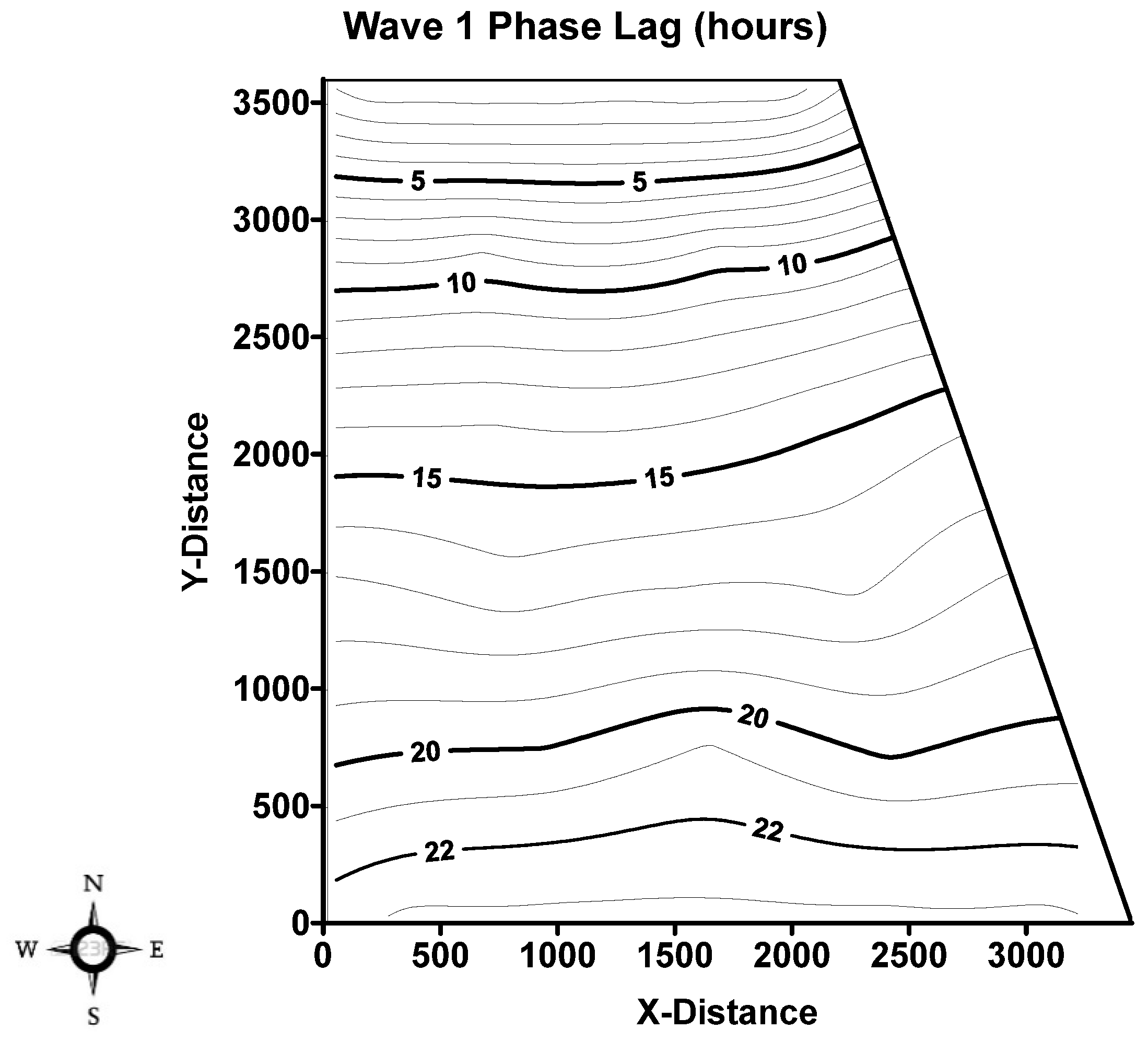
Phase lag contours for Wave 1 reached the wetland outflow structure in a little more than 23 h (Figure 4). Even though contour lines indicated that Wave 1 phase lags were the same across the width of Cell 2A, delay time changed downstream as vegetation density (hence resistance) changed, particularly near the outflow structures (e.g., 20 and 22 h contour lines). Contour lines reached the outflow structures at the same time, indicating uniform flow similar to a plug flow type. Previous research concluded that a plug flow type is an optimal design criterion to achieve high phosphorus performance in wetlands [9]. Part 2 of this research will discuss in detail how this flow type in STA3/4 led to better P retention compared to the SAV-dominated wetland (STA-2) characterized by myriad short circuits. The contour map of wave attenuation provides additional confirmation that K values are useful to represent vegetation resistance in large wetlands (Figure 5).

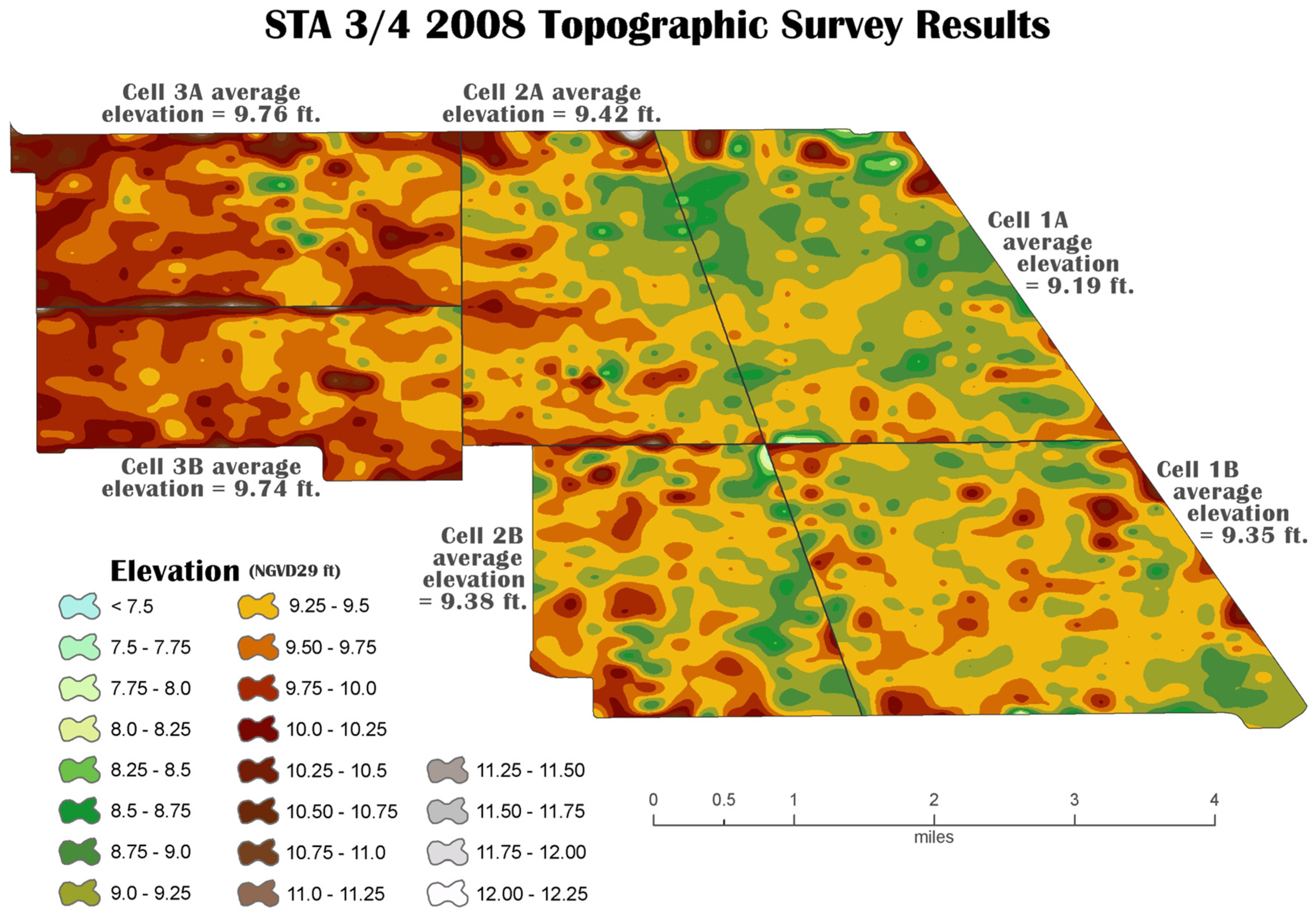
The Wave 1 amplitude attenuation (i.e., amplitude ratio) contour map (Figure 5) depicted the same trend observed in phase lag contour maps (Figure 4) and showed that total resistance (due to EAV) caused more attenuation near the center compared to the eastern side of the wetland (Figure 5). The amplitude ratios lagged along the eastern side, compared to the central pathway in the wetland. However, midway (between inflow and outflow structures), amplitude ratios along the eastern side were ahead of the central and western pathway. The elevation map of Cell 2A shows that higher bottom elevations are higher along the western side of the cell (Figure 9). It should be noted that the two contour maps represent different years (Figure 4/2014 vs. Figure 9/2008). Both observations (phase lags and amplitude attenuations) indicate that attenuations of wave amplitudes could be attributed to denser vegetation in the top half near the inflow structure of the cell and then less vegetation density in the bottom half of the cell. Furthermore, Wave 1 amplitude attenuation at the outflow structure was approximately 0.46 of the original signals, confirming that the selected wave frequency accurately penetrated the entire length of the wetland and still had an amplitude ratio greater than 0.20 of the original amplitude.

The vegetation density index map represents the best available information regarding EAV for current conditions in STAs (Figure 6, Figure 7 and Figure 8). Further research is needed to investigate how to better quantify EAV and SAV in terms of needed information (e.g., plant density, stem diameter, etc., or collectively “vegetation porosity”) and estimate vegetation resistance. The bulk values of K and a were obtained using Equations (9) and (10), with the knowledge of k₁ (Equation (7)) and k₂ (Equation (8)) calculated directly from field observations and can be used to determine existing flow types in a wetland (

Table A6. Identifying flow type (porous media, transitional, or surface water/weir flow) based on k₂ and k₁ ratios. If k₁/k₂ ≤ 0.2, the hyperbolic part of the PDE is dominant (surface water), and if k₁/k₂ > 0.9, the parabolic part of the PDE is dominant (i.e., porous media flow; loose gravel for example), and these equations can be simplified to K = f₂/(2k₁²) and C = f₂/k₂ [3]. Gray rows identify values where k₁/k₂ ≤ 0.2.

Gauges	Wave 1		Wave 2		Wave 3
	k1/k2	Flow Type	k1/k2	Flow Type	k1/k2	Flow Type
G377T-St04	0.15	1	0.22	1	0.21	1
St04-St03	0.49	2	0.52		0.54
St03-St02	0.51	2	0.45		0.36
St02-St01	0.59	2	0.83	2	0.19	1
St01-G378H	0.29	2	0.89	2	0.65
G377T-St14	0.16	1	0.21	1	0.30
St14-St13	0.47	2	0.59		0.49
St13-St12	0.61	2	0.41		0.30
St12-St11	0.48	2	0.61		0.20	1
St11-G378H	0.33	2	0.98	2	0.62
G377T-St24	0.22	1	0.29		0.28
St24-St22	0.49	2	0.53		0.44
St22-St21	0.44	2	0.33		0.19	1
St21-G378H	0.21	1	1.26	2	0.51
G377T-St34	Missing
St34-St32	0.43	2	0.41		0.34
St32-St-31	0.47	2	0.50		0.08	1
St31-G378H	0.33	2	0.92	2	0.41
G377T-St44	0.27	2	0.36		0.34
St44-St43	0.34	2	0.43		0.54
St43-St42	0.54	2	0.47		0.03	1
St42-St41	0.78	2	0.77		0.07	1
St41-G378H	0.14	1	0.83	2	0.55

).

Further research is needed to investigate how to better determine/quantify EAV and SAV in terms of needed information (e.g., plant density, stem diameter, etc., or collectively “vegetation porosity”) and estimate vegetation resistance. While it is important to fully understand and describe large wetland hydraulics, it is far more important to know and have the ability to describe flow type and how water flows inside those large features can be used to identify areas with less vegetation (open water areas) fast-moving water, less contact time, and hence less P uptake. The sole purpose for constructing large wetlands is to optimize nutrient retention, particularly P. Field experiments combined with available technology (e.g., remote sensing through drones to produce the vegetation index), which may provide a feasible way to determine areas of short circuiting and flow type in a large, constructed wetland to enhance P performance in those large, constructed wetlands.

5. Conclusions

The results of the wave propagation tests, conducted at three different discharge levels, showed that a new parameter set is needed to explain the wave behavior at each level. The results also showed that parameter values in the power functions are different for different flow regimes yet were remarkably similar to previous field experiment results and provided additional confirmation that the methods used to obtain vegetation resistance parameters (α and γ, K) were accurate.

Field observations from the wave test were used to quantify vegetation resistance in wetlands in terms of hydraulic transmissivity, a single parameter representing vegetation resistance. Analytical approaches to solve shallow water equations were used to calculate propagation and attenuation using inverse methods. The results showed that hydraulic transmissivity is a single quantifiable parameter that can represent bulk vegetation resistance in large, constructed wetlands, independent of vegetation type and prevailing flow type or conditions. This new single parameter was consistent and in agreement with the vegetation density/vegetation index, further indicating its reliability in estimating the effect of vegetation density on water flow and identifying areas of short circuiting to further enhance P removal. The proposed approach can also be used to represent bulk vegetation resistance in wetland model applications.

The objective of this study was to investigate how vegetation affects water flow and phosphorus retention in STAs. To accomplish this objective, we used sinusoidal discharge waves to measure water movement through wetland vegetation and developed a new single parameter (transmissivity K) to represent vegetation resistance. K values effectively indicated vegetation density, where high K represented low vegetation density/resistance, and low K represented high vegetation density/resistance; K proved consistent across different flow conditions and vegetation types. The method described in this research is more practical than traditional vegetation measurement methods, applicable across different vegetation types, consistent with vegetation density observations, and useful for modeling wetland hydraulics. This research demonstrated a novel way to measure and represent vegetation resistance in large, constructed wetlands, with practical applications for improving wetland performance in phosphorus removal. This method also provides a cost-effective way to assess wetland hydraulics and can help in optimizing phosphorus retention by identifying areas of fast water movement (less P retention) and areas of slow water movement (more P retention), which are useful for wetland design and management. The wave method also revealed areas of short circuiting, flow patterns through vegetation, and vegetation density distribution, all of which is very useful for wetland design and management.

References

1. Vymazal, J. Removal of nutrients in constructed wetlands for wastewater treatment through plant harvesting—Biomass and load matter the most. Ecol. Eng. 2020, 155, 105962. [Google Scholar] [CrossRef]
2. McCormick, P.V.; O’dell, M.B.; Shuford, R.B.; Backus, J.G.; Kennedy, W.C. Periphyton responses to experimental phosphorus enrichment in a subtropical wetland. Aquat. Bot. 2001, 71, 119–139. [Google Scholar] [CrossRef]
3. SFWMD. South FL Environmental Report and Other Publications. 2020. Available online: https://www.sfwmd.gov/science-data/scientific-publications-sfer (accessed on 15 May 2024).
4. SFWMD. Science Plan for the Everglades Stormwater Treatment Area. 2018. Available online: https://www.sfwmd.gov/sites/default/files/documents/rs_scienceplan_update_july2018.pdf (accessed on 15 May 2024).
5. Moustafa, M.Z.; Lal, A.M.W. Does Vegetation Resistance Impacts Phosphorus Performance in Large Constructed Wetlands? A Field Experiment Approach Part 1, Hydrology. Water, 2021; submitted. [Google Scholar]
6. Danckwerts, P.V. Continuous flow systems: Distribution of residence times. Chem. Eng. Sci. 1995, 50, 3857–3866. [Google Scholar] [CrossRef]
7. Dierberg, F.E.; DeBusk, T.A.; Jackson, S.D.; Chimney, M.J.; Pietro, K. Submerged aquatic vegetation-based treatment wetland for removing phosphorus from agricultural runoff: Response to hydraulic and nutrient loading. Water Res. 2002, 36, 1409–1422. [Google Scholar] [CrossRef]
8. Conn, R.M.; Fiedler, F.R. Increasing Hydraulic Residence Time in Constructed Stormwater Treatment Wetlands with Designed Bottom Topography. Water Environ. Res. 2006, 78, 2514–2523. [Google Scholar] [CrossRef] [PubMed]
9. Lee, J.K.; Roig, L.C.; Jenter, H.L.; Visser, H.M. Drag coefficients for modeling flow through emergent vegetation in the Florida Everglades. Ecol. Eng. 2004, 22, 237–249. [Google Scholar] [CrossRef]
10. Kadlec, R.H.; Wallace, S. Treatment Wetlands, 2nd ed.; CRC Press: Boca Raton, FL, USA; Taylor & Francis Group, LLC: London, UK; New York, NY, USA, 2009. [Google Scholar]
11. Dierberg, F.E.; DeBusk, T.A.; Henry, J.L.; Jackson, S.D.; Galloway, S.; Gabriel, M.C. Temporal and spatial patterns of internal phosphorus recycling in a South Florida (USA) stormwater treatment area. J. Environ. Qual. 2012, 41, 1661–1673. [Google Scholar] [CrossRef] [PubMed]
12. Kadlec, R.H. Detention and mixing in free water wetlands. Ecol. Eng. 1994, 3, 345–380. [Google Scholar] [CrossRef]
13. Lal, W.A.; Moustafa, M.Z.; Wilcox, W.M. The Use of Discharge Perturbations to Characterize In-Situ Vegetation Resistance; South Florida Water Management District: West Palm Beach, FL, USA, 2013.
14. Lal, A.M.; Moustafa, M.Z.; Wilcox, W. The use of discharge perturbations to understand in situ vegetation resistance in wetlands. Water Resources. Res. 2015, 51, 2477–2497. [Google Scholar] [CrossRef]
15. Lal, A.W. Mapping Vegetation Resistance Parameters in Wetlands Using Generated Waves. J. Hydraul. Eng. 2017, 143, 04017023. [Google Scholar]
16. Kuester, J.L.; Mize, J.H. Optimization Technique with Fortran; McGraw Hill: New York, NY, USA, 1973. [Google Scholar]
17. Zinke, P. Application of Porous Media Approach for Vegetation Flow Resistance. In River Flow; Munoz, R.M., Ed.; CRC Press: London, UK, 2012; pp. 301–307. [Google Scholar]
18. Green, J. Comparison of blockage factors in modeling the resistance of channels containing submerged macrophytes. River Res. Applic. 2005, 21, 671–686. [Google Scholar] [CrossRef]
19. Martinez, C.J.; Wise, W.R. Analysis of constructed treatment wetland hydraulic with the transient storage model OTIS. Ecol. Eng. 2003, 20, 211–222. [Google Scholar] [CrossRef]
20. Hammond, D.S.; Chapman, L.; Thornes, J.E. Roughness length estimation along road transects using airborne LIDAR data. Met. Apps. 2012, 19, 420–426. [Google Scholar] [CrossRef]
21. Moustafa, M.; Wang, N. Assessment of wind and vegetation interactions in constructed wetlands. Water 2020, 12, 1937. [Google Scholar] [CrossRef]
22. South Florida Engineering and Consultants (SFEC). Sustainable Landscape and Treatment in a Stormwater Treatment Area Study, Final Report (C-4600004015-WO09); South Florida Engineering and Consultants (SFEC): Lake Worth Beach, FL, USA, 2024. [Google Scholar]
Figure 1. Stormwater Treatment Area locations and field experiment sites. Panel (A): locations of all STAs south of Lake Okeechobee, containing emergent aquatic vegetation (EAV) and submerged aquatic vegetation (SAV). Blue areas (AC) represent location of Flow Equalization Basins (FEB) to supply water to STAs during dry seasons. Vegetation is used to reduce phosphorus in surface water, prior to entering the Everglades Protection Area. Panel (B): dominant vegetation types in STAs. EAV represented by a light green color and SAV depicted in a light blue color. Panel (C): STA2C3 with water level logger locations (red pins) and inflow and outflow structures (green triangles). Panel (D): STA34C2A with water level logger locations (red pins) and missing loggers (stars inside yellow markers) and permanent stage data recorder (yellow pin).
Water 17 00266 g001aWater 17 00266 g001b
Figure 2. (A) Schematics of study areas depict canals and structures used to route water into study sites. STA4C2A was dominated by EAV during the study. Blue and pink colors represent water supply canals. (B) Field experiment gauge locations in study sites (STA34C2A). Light-gray circles indicate in situ water level logger locations during the field experiment. Dark-gray square markers indicate inflow and outflow structures (G-377 and G-378). Both G378-T and G-378H are permanent-stage data recorders inside the wetland. Dark and light gray arrows represent inflow and outflow discharge directions.
Water 17 00266 g002
Figure 3. Ponding/flat pool test: no inflow and or outflow discharges for 2–3 days, which determines the point at which both upstream and downstream stage reading are identical. Stage reading at this point determines the adjustment that needs to be made for all sensors.
Water 17 00266 g003
Figure 4. Contour map of phase lag in hours in STA34C2A for Wave 1 inside the study area.
Water 17 00266 g004
Figure 5. Contour map of wave amplitude attenuation ratios in ST34C2A for Wave 1 inside the study area.
Water 17 00266 g005
Figure 6. Contour map of transmissivity (K = m2·s−1) overlaid on a map representing the vegetation index in STA34C2A for Wave 1. A high vegetation index indicates higher vegetation density, located in areas with low K values (western side), while a high K value indicates less vegetation resistance and is located in areas with a low vegetation index (eastern side).
Water 17 00266 g006
Figure 7. Contour map of transmissivity (K = m2·s−1) overlaid on a map representing the vegetation index in STA34C2A for Wave 2. A high vegetation index indicates higher vegetation density, located in areas with low K values (western side), while a high K value indicates less vegetation resistance and is located in areas with a low vegetation index (eastern side).
Water 17 00266 g007
Figure 8. Contour map of transmissivity (K = m2·s−1) overlaid on a map representing the vegetation index in STA34C2A for Wave 3. A high vegetation index indicates higher vegetation density, located in areas with low K values (western side), while a high K value indicates less vegetation resistance and is located in areas with a low vegetation index (eastern side).
Water 17 00266 g008
Figure 9. Map of Cell 2A bottom elevations. High bottom elevations (9.5 to 10 ft NGVD) are on the western side, while higher elevations (>10 ft NGVD) are near the inflow discharge structure. The central and eastern side of Cell 2A is dominated by lowest bottom elevations (8.5 to 9.5 ft NGVD). This DEM was created using a 500′ × 1000′ grid of survey data points. Some of the microtopography is a result of the survey data point locations and the method used to create DEM. In other words, the bottom is not exactly as shown in the DEM. Instead, this is a general representation of the topography that was used to estimate the average ground elevation.
Water 17 00266 g009
Disclaimer/Publisher’s Note: The statements, opinions and data contained in all publications are solely those of the individual author(s) and contributor(s) and not of MDPI and/or the editor(s). MDPI and/or the editor(s) disclaim responsibility for any injury to people or property resulting from any ideas, methods, instructions or products referred to in the content.