Article

Impacts of the Degree of Heterogeneity on Design Flood Estimates: Region of Influence vs. Fixed Region Approaches

1
School of Engineering, Design and Built Environment, Building XB, Western Sydney University, Kingswood, Penrith 2747, Australia
2
Department of Civil Engineering, Ahsanullah University of Science and Technology, Dhaka 1208, Bangladesh
3
Department of Electrical and Computer Engineering, North South University, Dhaka 1229, Bangladesh
4
CSIRO Environment, Canberra 2601, Australia
5
Department of Civil Engineering, Indian Institute of Technology, Kharagpur 721302, West Bengal, India
*
Author to whom correspondence should be addressed.
Water 2025, 17(18), 2765; https://doi.org/10.3390/w17182765
Submission received: 5 July 2025 / Revised: 1 September 2025 / Accepted: 11 September 2025 / Published: 18 September 2025

Abstract

In regional flood frequency analysis (RFFA), the formation of homogeneous regions is commonly regarded as a necessary condition for reliable regional flood estimation. However, achieving true homogeneity is often challenging in practice. This study investigates the formation of homogeneous regions by applying two region delineation approaches—fixed regions and the region-of-influence (ROI) method—accompanied by the widely used heterogeneity measure (H1) proposed by Hosking and Wallis. The analysis utilizes data from 201 stream gauging stations across southeast Australia, evaluating a total of 1211 candidate regions. The computed H1-statistics range from 13 to 30 for fixed regions and from 6 to 30 for ROI-based regions, indicating a consistently high level of heterogeneity across the study area. This suggests that the assumption of homogeneity may not be realistic for many parts of southeast Australia. Moreover, regression equations developed for regional flood estimation yield absolute median relative errors between 29% and 56%, with a median of 39% across return periods from 2 to 100 years. These findings underscore the limitations of relying solely on homogeneity in regional flood modelling and highlight the need for more flexible and robust approaches in RFFA. The outcomes of this research have significant implications for improving flood estimation practices and are expected to contribute to future enhancements of the Australian Rainfall and Runoff (ARR) national guidelines.

1. Introduction

Floods are one of the worst natural disasters globally. A probabilistic approach is used when designing flood-safe hydraulic structures, where a streamflow is linked with an annual exceedance probability (AEP) or return period (T) to find a design flow, such as 100-year flood. At a location of interest where good quality streamflow data are available, at-site flood frequency analysis (FFA) is widely adopted; however, for sites with no/little streamflow data, regional flood frequency analysis (RFFA) is adopted to estimate design floods [1,2]. In RFFA, data from similar sites are pooled to develop prediction models [3].
A group of catchments exhibiting similar hydrological responses may form a homogeneous region [4]. Among all the RFFA techniques, the index flood method is widely used, which heavily relies on the concept of homogeneous regions [5,6]. As per the index flood method, a group of stations forms a homogeneous region if their standardized flood frequency curves are like each other within a certain margin of sampling variability [5]. In contrast, the quantile regression technique (QRT), another type of RFFA method, relaxes the homogeneity assumption, i.e., it does not need a perfect homogeneous region [7]. However, there is a notion in RFFA that even in QRT, if the regions are homogeneous, the prediction error will be smaller [4]; however, this has never been tested thoroughly, e.g., in Australia.
Traditionally, a fixed-region approach is applied to identify regions in RFFA for simplicity [2]. A statistical criterion, such as the regional homogeneity test by Hosking and Wallis [5], is generally applied to evaluate the level of homogeneity of an assumed region. Numerous studies have explored the formation of homogeneous regions in RFFA [8,9,10].
In contrast to regions formed on geographical space, regions can also be formed in the hydrological and basin attributes space. Cluster analysis and principal component analysis (PCA) are generally adopted to form these regions in a catchment attributes space [11,12].
The fixed-region approach often lacks in homogeneity. To overcome the limitations of the fixed-region approach, the region-of-influence (ROI) approach is proposed, where a local region is formed around each of the selected stations in the geographic or catchment attributes space [3,13]. The ROI approach has successfully been applied to many RFFA studies [14]. The ROI approach generally outperforms the fixed-regions approach in RFFA [15,16,17,18].
Spatial proximity-based ROI generally outperforms the purely fixed-region approach where all the stations in a country/state are placed in a fixed region [19,20]. In the Gulf-Atlantic Rolling Plains of the United States, a 50-year flood quantile was regionalised based on the principle of geographical proximity. Here, the ROI outperformed the fixed-region approach for both geographic and catchment attributes space [19]. Similarly, using 204 stations in Arkansas, the ROI approach was found to outperform five other RFFA techniques [21]. In Québec and Ontario, the Canadian Statistical Hydrology Research Group compared four different RFFA frameworks and five distinct RFFA methods. Using the regional hydrological attributes as inputs to identify homogeneous regions and to enhance the efficiency of analysis, a novel regionalisation process called the Automatic Region Revision Algorithm (ARRA) was formulated, which was complementary to both the L-moments-based and the ROI approaches [5].
A few studies have noted that successful identification of homogeneous regions is dependent on the hydrological features of the sites [22].
Although there have been many studies in RFFA, no single method is available that can be confidently applied across all countries to identify homogeneous regions. There has been no success on the identification of acceptable homogeneous regions in Australia using traditional homogeneity tests. Moreover, there has been a limited number of studies on how the degree of heterogeneity impacts the model accuracy in RFFA in a QRT framework. Our research intends to fill this knowledge gap by assessing the regional heterogeneity of catchments in southeast Australia using both the fixed-region and ROI approaches and quantifying the impacts of level of regional homogeneity on the design flood estimates in a QRT framework.

2. Data and Methodology

2.1. Selection of Study Area

Southeast Australia (Victoria (VIC) and New South Wales (NSW)) is selected as the study area, as the streamflow gauging network is dense in this part of Australia. A total of 201 stations is selected from these two Australian states (Figure 1). The selected catchments are predominantly natural and have no significant storage and land use change, and these are small to medium in size. This part of Australia is significant, as most of the people in Australia live here; hence, significant capital investment is made. For most of these investments, flood risk assessment is needed, as the investments are situated in flood plains. The mean annual rainfall in the study area ranges from 470 mm to 1950 mm, while the mean annual potential evapotranspiration varies from 900 mm to 1550 mm. The Great Dividing Range (GDR) separates coastal areas from the inland plain areas. The rivers located to the east or southeast of the GDR fall to the adjacent sea, while the rivers on the inland side flow to the Murray Darling basins.
Table S1 (in Supplementary Section) provides important physical features and statistical indices of the selected 201 catchments, such as the discordancy measure (Di) (any Di > 3 indicates a discordant site as per Hosking and Wallis [5] criteria). Figure S1 presents cluster analysis (by Ward’s method) results where three catchment groups (Group 1, Group 2 and Group 3) are formed (sites are labelled by site index, column 1 of Table S1). Figure S2 exhibits the hydrological perspectives of these three clustering groups where it is found that Group 1 is dominated by smaller LCV (of AMF data) values, Group 3 is dominated by higher LCV values, and Group 2 is characterized by moderate LCV values.
The selection of stations and catchment characteristics in RFFA generally relies on some basic recommendations. The selected catchment characteristics should have (i) a direct impact on flood response (in flood generation mechanism), (ii) easy accessibility, (iii) proper definition, (iv) simple physical explanation, (v) no major correlation among them (i.e., avoiding highly correlated characteristics), and (vi) better prediction performance.
Based on the relevance to previous studies in Australia, eight climatic and catchment characteristics are selected for this study (shown in Table 1). The data for these characteristics were obtained from the Australian Bureau of Meteorology (BoM) website and Australian Rainfall and Runoff Revision Project 5 Regional flood methods. Table 1 summarises the basic statistics of the catchment characteristics data of the selected 201 stations. With a mean of 333.99 km2, the AREA values lie in a range from 3.00 to 1010.00 km2 (standard deviation: 262.40 km2). The AREA of the maximum stations (n = 138, ~69%) is within 3 to 400 km2, and only one station has an AREA of 1010 km2. The MAR values range from 484.39 to 1953.23 mm, with a mean of 962.26 mm and the median of 891.64 mm (standard deviation (SD) = 314.47 mm). I62 and MAE are extracted from the BoM website. The highest and the lowest values for the predictor I62 are 87.30 and 24.60 mm/h (SD = 10.07 mm/hr), respectively. In case of MAE, these figures are 1543.30 and 925.90 mm (SD = 129.31 mm), respectively. The length of time AMF data have been recorded (record length) is in the range 25.00 to 89.00 years (mean = 45 years and SD = 9.63 years). Out of 201 stations, roughly 68% (n = 137) of stations have a record length of 40 to 50 years for AMF data.

2.2. Formation of Regions

By placing all the 201 selected stations, a single fixed region (A) is formed. Thereafter, considering the administrative boundaries, i.e., based on the states (NSW and VIC), the selected stations are divided into two fixed regions (B1 and B2). In a different way, based on the drainage division (DD), the stations are grouped into two regions. Stations with station identification numbers (SINs) starting with ‘2’ (stations falling in DD 2) are placed in one region (C1), and stations with SINs starting with ‘4’ are placed in another region (C2). Lastly, the ROI approach is used to form regions where the KNN (K-nearest neighbour) principle is adopted, with 10, 20, 50, 100, 150, and 200 nearby stations being selected around each of the 201 stations. A summary of the assumed regions with their notation and number of stations in each region can be found in Table 2.

2.3. Evaluation of Homogeneity of the Selected Regions

In RFFA, various types of heterogeneity tests have been introduced; however, the most widely used one is the L-moments-based test by Hosking and Wallis [5], which is adopted in this study. For a homogeneous region, population L-moments will be the same for all the sites in a proposed region; however, their sample L-moments will be different [5]. To assess the degree of sampling variability, Hosking and Wallis [5] used simulation based on a four-parameter Kappa distribution. Based on the results of this simulation, three statistics were proposed to evaluate regional homogeneity. These are (i) the discordancy measure (Di) for detecting discordant stations, (ii) the heterogeneity measure (Hi) for finding the degree of homogeneity in a region, and (iii) the goodness-of-fit measure (|Z|-statistics) for selecting the best fit distribution(s) for the assumed region. Based on the dimensionless L-moment coefficients (LCV, LSK, and LKUR), the Hi -statistics (i = 1 to 3) are generated [5].
The discordancy measure (Di) can be expressed as
D i = 1 3 ( u i u ¯ ) T   S 1 ( u i u ¯ )
where ui represents the vector of LCV, LCS, and LCK for a station i
S = covariance matrix of ui, ū = mean of vector ui.
If Di ≥ 3.00, a station is said to be discordant.
Assuming the station i has the record length ni and sample L-moment ratios are t(i), t3(i), and t4(i), the regional average LCV, LSK, and LKUR are weighted by the stations’ record length and are presented as tR, t3R and t4R, respectively. Mathematically,
t R = Σ n i t i i = 1 n i
and the weighted standard deviation can be estimated by
V = [ Σ n i ( t i t R ) 2 i = 1 n i ]
Finally, a heterogeneity measure, the H-statistic, can be estimated as
H = ( V µ v ) σ v
Here, µ v   and σ v represent the mean and standard deviation of the simulated values, respectively, and V represents the weighted standard deviation of simulated values. The following rules are used to evaluate the homogeneity:
  • H < 1: a proposed region is regarded as acceptably homogeneous;
  • 1 ≤ H < 2: a proposed region is possibly heterogeneous;
  • H ≥ 2: a proposed region is regarded as definitely heterogeneous.
Z-distribution is defined as
Z Dist = 1 σ 4 [ τ 4 Dist ( t   bar ) 4 + β 4 ]
where σ 4 = standard deviation of L-kurtosis values obtained from simulation,
τ4Dist = average L-kurtosis value computed from simulation for the fitted Kappa distribution,
(t bar)4 = average L-kurtosis value computed from the data of a given region, and β4 = bias of τ4.
A distribution is regarded the best fit for the assumed region if the |Z|-statistic value is ≤1.64 [5].

2.4. Regional Estimation Model Development

The quantile regression technique (QRT) is applied for developing a prediction equation for a given region and for a given return period [23]. The QRT is defined by
QT = aBbCcDd
where QT is a flood discharge with 1 in T AEP, B, C, D, … are predictors, and a, b, c, … are the regression coefficients, which are estimated by the method of ordinary least squares (OLS).
Using the logarithmic (base 10) transformation and applying the selected predictors (see Table 1), the QRT can be expressed as
l o g 10 ( Q T ) = b 0 + b 1 ×   l o g 10 ( A R E A ) + b 2 × l o g 10 ( I 62 ) + b 3 × l o g 10 ( M A R ) + b 4 × l o g 10 ( S F ) + b 5 × l o g 10 ( M A E ) + b 6 × l o g 10 ( S D E N ) + b 7 × l o g 10 ( S 1085 ) + b 8 × l o g 10 ( F O R E S T )
where QT is the flood quantile for the T-year return level. These QT values were calculated from fitting a log-Pearson Type 3 (LP3) distribution to the AMF data at each of the 201 selected stations. FLIKE software (TUFLOW Flike 5.0.220.0) was used to fit the LP3 distribution to the AMF data [24]. The reason for using LP3 distribution is that previous Australian studies found LP3 to be the suitable distribution to describe AMF data for most Australian streamflow gauging stations.

2.5. Evaluation Criteria

To validate the developed prediction equation, six statistical indices were adopted: (i) relative error (RE), (ii) mean square error (MSE), (iii) bias (BIAS), (iv) relative bias (RBIAS), (v) relative root mean square error (RRMSE), and (vi) root mean square normalized error (RMSNE).
R E = Q p r e d Q o b s Q o b s × 100
M S E = m e a n Q p r e d Q o b s 2
B I A S = m e a n Q p r e d Q o b s
R B I A S = m e a n Q p r e d Q o b s Q o b s × 100
R R M S E = m e a n Q p r e d Q o b s 2 m e a n [ Q o b s ]
R M S N E = [ m e a n Q p r e d Q o b s Q o b s 2 ]
Here, Qpred is obtained by the RFFA model derived in this study and Qobs is estimated by FFA, as noted before. A leave-one-out (LOO) validation method is considered here, where each of the selected stations is tested by applying the developed prediction, derived without the test station. Absolute median relative error (AMRE) is calculated as the median of the absolute RE values of all the selected stations to provide an overall model error estimate. R was used for carrying out the regression analysis.

3. Results

3.1. Exploratory Analysis

To understand hydrological perspectives of the catchment groups, three clustering groups (Figure S1) are formed based on catchment characteristics data; these groups are then linked to the LCV values of the AMF data of the selected stations in Figure S2. This figure clearly exhibits the differences in the LCV values of the three clustering groups. For example, Group 1 has much smaller LCV values than Group 3.
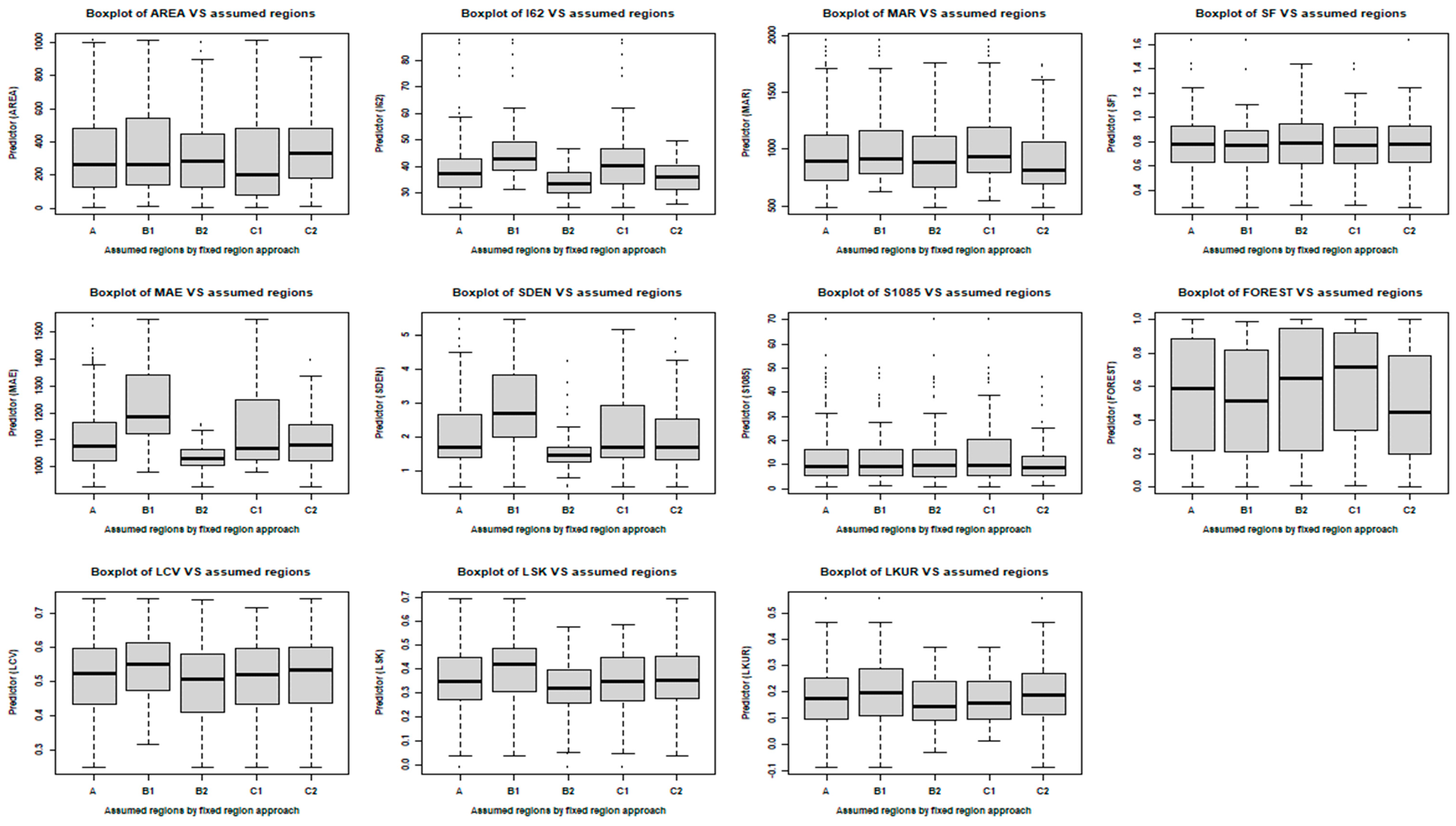
The predictor variables and L-moments for the fixed regions are represented by boxplots in Figure 2. It can be seen that fixed-region A is characterized by the second-highest median AREA, I62, MAR, MAE, and FOREST, and smaller SDEN values, which implies a region with comparatively larger, wetter, more forested, and stepper stations. In contrast, fixed-region B1 has the highest median I62, MAR, MAE, and SDEN and almost similar S1085. It also has the and second-lowest FOREST values. These characteristic suggest a group of wet, steeper, and relatively less-forested stations. The median L-moment (LCV, LSK, and LKUR) values become higher in this region. Region B2 has the smallest median I62, MAE, and SDEN and the second-lowest FOREST values, which points to a group of drier and stepper stations with larger forest cover, thus they have the lowest median L-moment values. Region C1 has the smallest median AREA and the highest median MAR and FOREST values, which implies a group of smaller, wetter, and more forested stations. In contrast, region C2 is dominated by the highest median AREA and the lowest median MAR and FOREST values (i.e., low forestation, dry and bigger catchments). The correlations among the eight predictor variables used in developing regression equations need to be examined. The Variance Inflation Factor (VIF) is used to measure the impact of the degree of multicollinearity on the regression results. Typically, VIF values above five indicate the presence of a significant multicollinearity. In the present study, all the VIF values are below four, suggesting a low level of multicollinearity, which is unlikely to affect the stability of our regression coefficients.

3.2. Discordancy, Heterogeneity, and Z-Statistics of the Assumed Regions

Table 2 shows the summary statistics of the assumed regions with their Di and Z-values. Here, the reported Di values are 3.00 or more. The lowest Di values fall in the range 3.05 (B1 and C2)–3.34 (C1) for the assumed fixed regions. Adopting the ROI approach, these values range from 3.07 (KNN50) to 3.62 (KNN150). In contrast, for the assumed fixed regions, the highest Di values range from 5.04 (B2) to 7.18 (C2), and for the ROI approach, this range is from 5.40 (KNN100) to 7.70 (KNN150). Interestingly, there are no discordant stations for both the KNN 10 and 20. As per Hosking and Wallis [5] criteria, the Z-values clearly indicate that Pearson Type three (PE3) and Generalized Pareto (GPA) are the most suitable regional distributions in the study area.

3.3. Discordancy and Comparison of Fixed Region and ROI Approaches in Identification of Homogeneous Regions

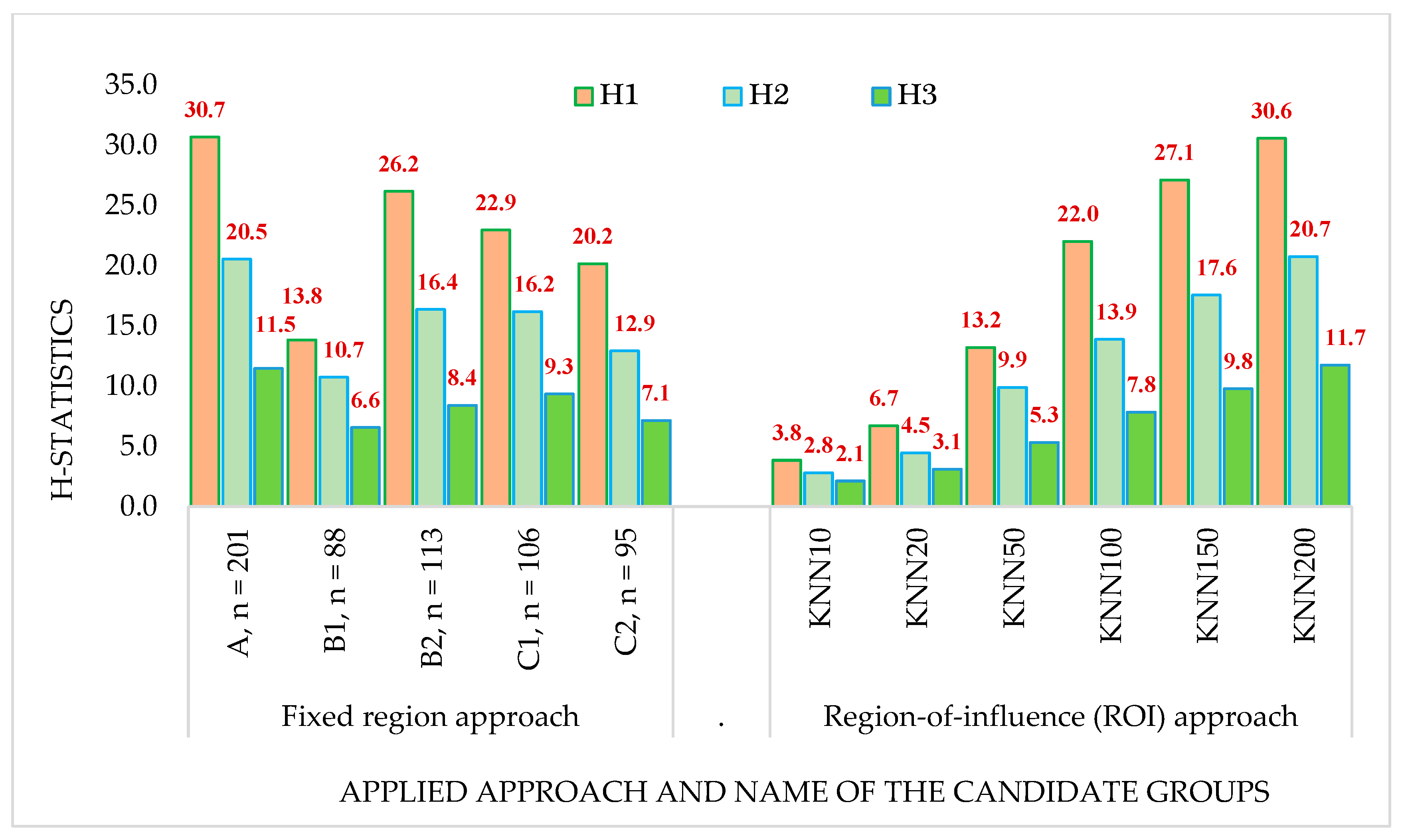
Figure 3 exhibits the distribution of calculated Hi (median values) for the considered fixed regions and regions based on the ROI approach. The H1-statistics range from 13.8 to 30.7 and 3.8 to 30.6 in the approaches, respectively. This clearly shows that the assumed groups are highly heterogeneous.
Adopting the fixed-region approach, in region A (n = 201), the calculated Hi-values (i = 1, 2, and 3) are the highest and vary from 11.5 to 30.7. However, the lowest Hi-values are observed in region B1 (n = 88), ranging from 6.6 to 13.8. With an exception for H3-values (in region C1); the second-, third-, and fourth-highest Hi-values are found in the regions B2 (n = 113), C1 (n = 106), and C2 (n = 95), respectively. These figures fluctuate from 8.4 to 26.2, 9.3 to 22.9, and 7.1 to 20.2. This indicates that the Hi-statistics gradually decrease with the decreasing number of stations. In addition, when applying the ROI approach, the Hi -statistics reveal the same notion. The lowest H1-value (3.8) is noted for KNN10, and it steeply increases for the higher-order KNNs. Eventually, the highest H1-statistic (30.6) is observed for KNN200. In this approach, the median H2-value ranges from 2.8 (for KNN10) to 20.7 (for KNN200), and the H3-value varies from 2.1 (for KNN10) to 11.7 (for KNN200). Having higher Hi-statistics, the relationship H1 > H2 > H3 is observed among the assumed regions. It is obvious from the graph that Hi-statistics sharply increase with the increased number of stations in a region formed using both the fixed-region and ROI approaches.
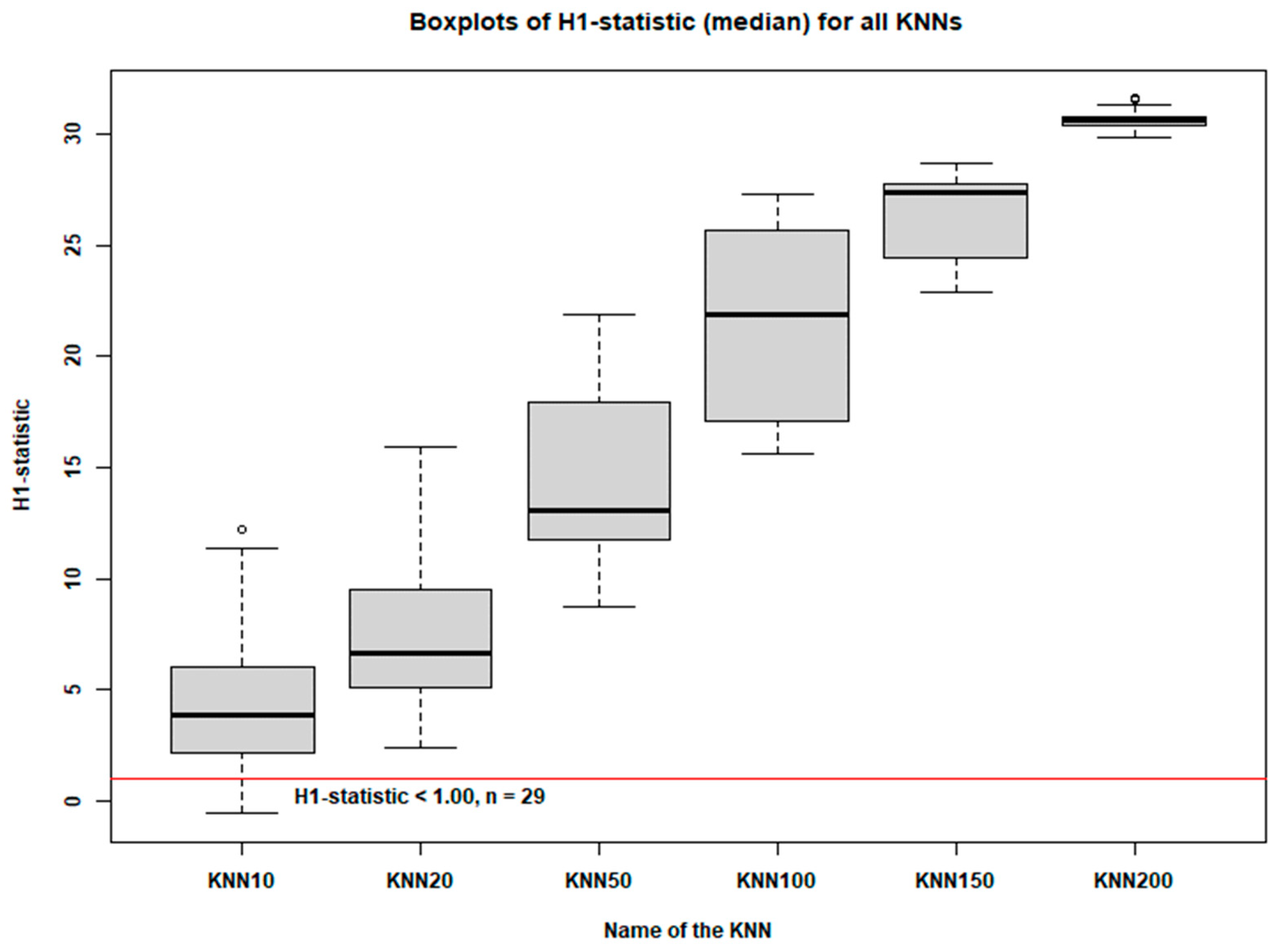
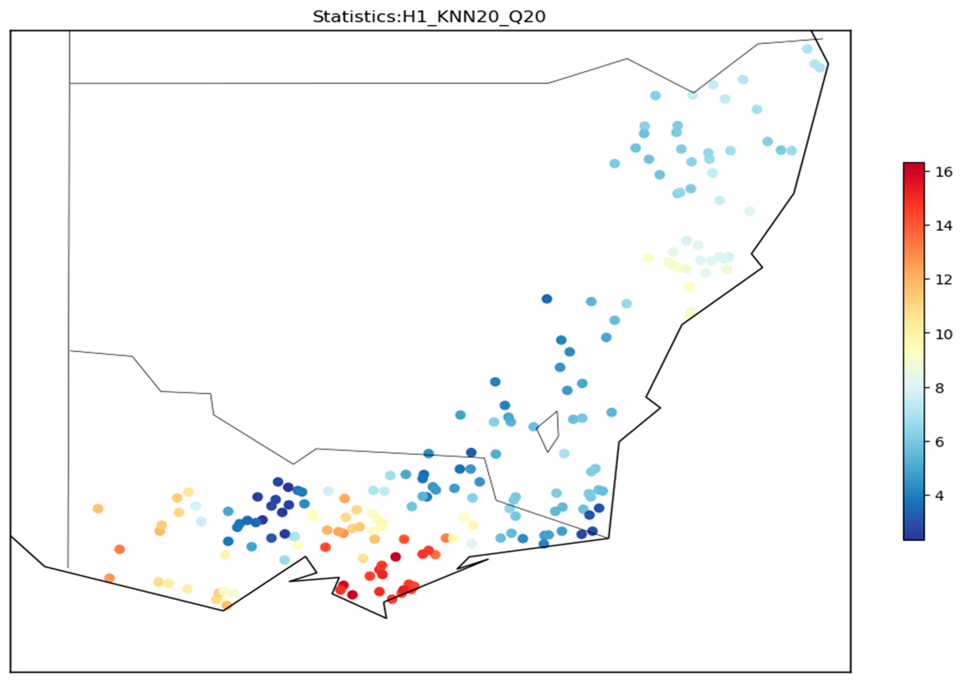
Despite these high Hi-statistics, 29 stations are identified as homogeneous regions (H1 < 1.00) only in the KNN10 approach (Figure 4, red colour). No other approaches identify any homogeneous region. Table S2 (Supplementary Section) shows a detailed summary of these homogeneous regions, including the target and member stations’ ID numbers and respective H1-values. Figure 5 shows an in-depth summary of the H1-values obtained using the ROI approach. More specifically, the spatial distribution in Figure 6 shows the magnitude of the H1-statistic for KNN20 for Q20. The spatial distribution of H1-statistics to estimate Q20, adopting ROI approach, can be found in the Supplementary Section (Figure S3 for KNN50 and Figure S4 for KNN100).
A comparison between the H1-statistics and absolute RE values for the KNN50, KNN100, and KNN150 approaches to estimate Q2, Q5, Q10, Q50, and Q100 can be found in Figures S5–S9 (see Supplementary Section), respectively.
To understand the temporal changes in homogeneity for different parts of the study area, each stations’ AMF data are divided into three parts: (i) full length, (ii) earlier part (till 1990), and (iii) most recent part (1991–2018). Figure 6, Figures S10 and S11 present the spatial distributions of H1-statistics for KNN20 for these three subsets of AMF data. For earlier AMF data (till 1990), southwest Victoria is dominated by a higher spatial homogeneity (marked by light blue colour) (Figure S10). In contrast, for the most recent AMF data (1991–2018), southwest Victoria is dominated by a higher level of heterogeneity (indicated by light-red to red colour) (Figure S11). However, for the full AMF data length, this part of Victoria is dominated by a moderate level of heterogeneity (indicated by the light-yellow colour) (Figure 6). This clearly demonstrates that more recent AMF flood data have higher variability (i.e., higher LCV), resulting in a higher degree of heterogeneity. Another distinct pattern is visible due to temporal variation in AMF data in the northeastern NSW, where earlier data (Figure S10) indicates a moderate spatial heterogeneity (light-yellow colour), and the most recent data (Figure S11) and the full AMF data (Figure 6) show a moderate level of spatial homogeneity. This indicates a shift towards a greater level of spatial homogeneity in northeast NSW over time. It is interesting to note that the mid-south Victoria (adjacent to Melbourne) exhibits the highest level of spatial heterogeneity (represented by deep red colour) for all the three AMF data subsets.

3.4. Comparison of Fixed-Region and ROI Approaches

3.4.1. Prediction Equation Development and Performance

Table 3 summarises the regression coefficients (based on equation 7) for Q50 for the assumed regions. This table also shows the adjusted coefficient of determinant (Adj-R2) values. Detailed descriptive statistics of the regression coefficients for all the quantiles are presented in the Supplementary Section (Table S3). Region KNN10 is not considered for further analysis as the number of stations in this region is < 20 (n = 15).

3.4.2. Assessment of the Impact of Homogeneity on Prediction Accuracy

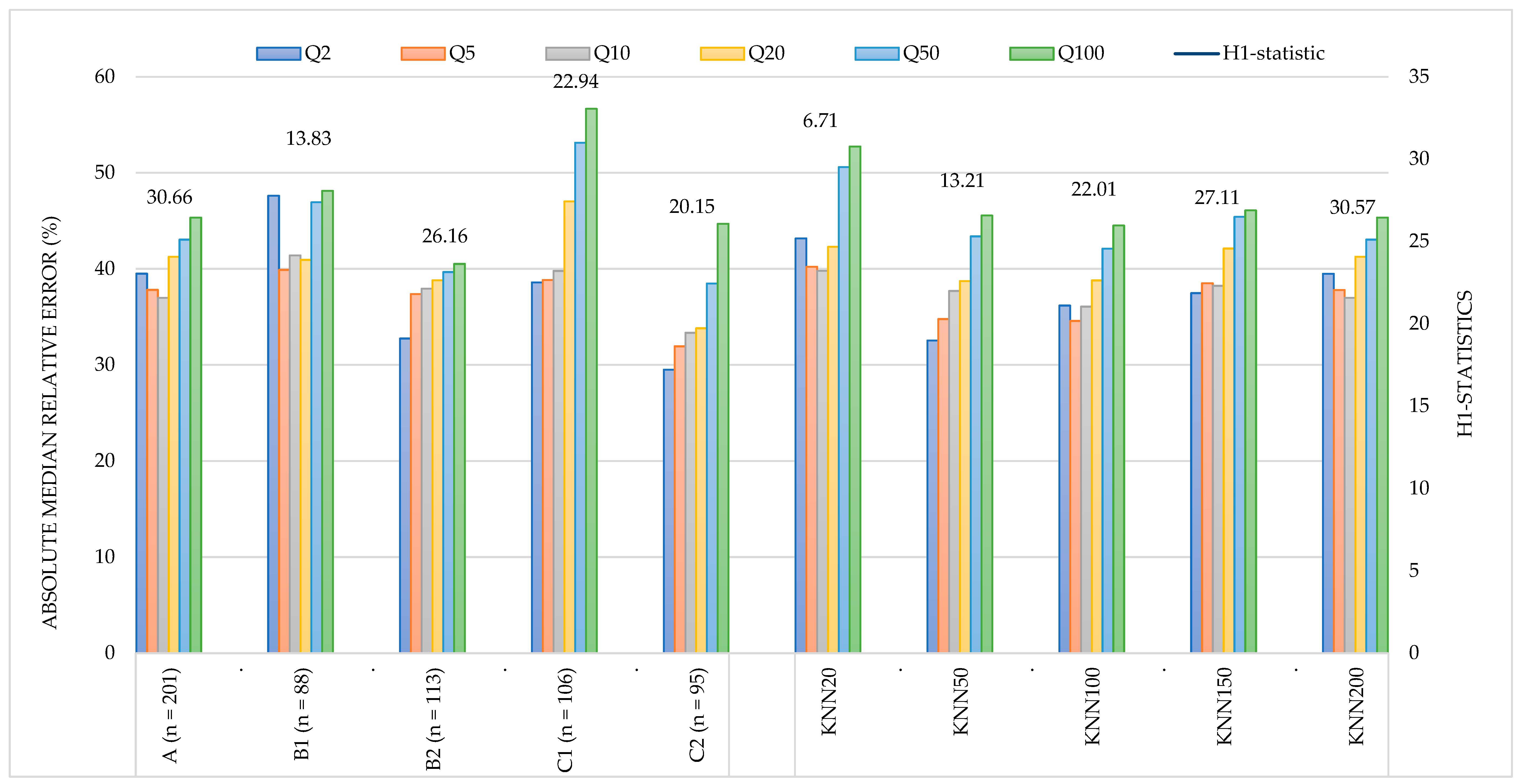
Figure 7 assesses the effects of the heterogeneity level on the prediction accuracy of the developed regional prediction equations (H1- vs. AMRE values). For the assumed fixed region A (n = 201), which has the highest H1-value (30.66), the AMRE values range from 36.98% (Q10) to 45.34% (Q100). Interestingly, using the ROI approach, the region KNN200 (n = 200) has the same AMRE values, with an H1-statistic of 30.57. With the lowest H1-value (6.71) the region KNN20 shows moderately high AMRE values. In this region, the minimum and the maximum AMRE values are 39.79% (Q10) and 52.73% (Q100), respectively. In contrast, having a higher H1-statistic (22.94), the region C1 (n = 106) also exhibits higher AMRE values, which range from 38.58% (Q2) to 56.66% (Q100). It is noted here that exhibiting the lowest (KNN20) and 5th highest (C1) H1-values, the regions have more than 50.00% AMRE values for Q50 and Q100. Similar to KNN200, the regions B1 (n = 88), B2 (n = 113), C2 (n = 95), KNN50, KNN100, and KNN150 have less than 49.00% AMRE values, with H1-statistics of 13.83, 26.16, 20.15, 13.21, 22.01, and 27.11, respectively. The lowest AMRE values are observed in the region B2 (VIC state); these values lie in a range from 32.74% (Q2) to 40.51% (Q100), with a relatively higher H1-value (26.16). In addition, compared to this figure, regions C2 (H1-value 20.15), KNN50 (H1-value 13.21), and KNN100 (H1-value 22.01) show lower AMRE values up to Q20. Figure 7 clearly indicates a poor relationship between the heterogeneity level and the prediction accuracy of the quantile estimates adopted from either the fixed-region or ROI approaches.
Table 4 shows the summary statistics of the evaluation criteria of the developed prediction equations for the assumed fixed regions and the regions based on the ROI approach. The R2 values of the formed fixed regions fluctuate from 0.53 (region B2 for Q100) to 0.80 (region C1 for Q2). Applying the ROI approach, these R2 values range from 0.58 (region KNN150 for Q100) to 0.84 (region KNN20 for Q2 and Q5). It is obvious from this table that with the increase in the return period the R2 values decreased (with the exception of the C2 region). Thus, there is an inverse relationship between the R2 values and the return period (T), as expected.
In the fixed regions, the lowest AMRE value is 29.50% (Q2 of region C2) and the highest is 56.66% (Q100 of region C1), with the overall median 39.72% (SD 6.06%). Likewise, adopting the ROI approach, the AMRE values are 32.53% (Q2 of region KNN50) and 52.73% (Q100 of region KNN20), respectively, with an overall median of 40.00% (SD 4.63%). Here, the SD values indicate that the ROI approach provides relatively more consistent and precise flood quantile estimates than the fixed-region approach.
In the assumed fixed regions, the minimum MSE value (613) is observed in region B2 for Q2 and the maximum (1,576,140) is in region B1 for Q100. The overall median and SD values of the MSE for these regions are 40,902 and 367,830, respectively. On the other hand, these MSE values are higher for the assumed regions formed by the ROI method. In this case, the highest and the lowest MSE values are 3,201,044 (Q100 of region KNN20) and 2476 (Q2 of region KNN150), respectively. The overall median and SD values of the MSE are 95,007 and 641,000, respectively. Among the assumed fixed regions, the BIAS ranges from −233.05 (Q100 of region B1) to −3.79 (Q2 of region B2), and in the ROI approach, it ranges from −169.16 (Q100 of region KNN200) to −6.33 (Q2 of region KNN50). Interestingly, only for the region KNN20 is the BIAS is positive, and it ranges from 1.68 (Q2) to 93.24 (Q100). Within the assumed fixed regions, the overall median and SD values of BIAS are −34.28 and 58.94, respectively. In case of the ROI approach, these figures are −20.25 and 50.09, respectively. This shows that the ROI outperforms the fixed-region approach to estimate the flood quantile in southeastern Australia. The estimated highest RBIAS values for the fixed-region and ROI approaches are 56.20 (Q100) and 68.05 (Q100) in the assumed regions B1 and KNN20, respectively. The lowest RBIAS values are 14.63 (Q5) and 21.41 (Q5) in the regions C2 and KNN200, respectively. In the assumed fixed regions, the overall median RBIAS is 27.33 (SD = 10.24), and for ROIs it is 31.22 (SD = 10.18). Adopting the fixed-region approach, the RRMSE values range from 0.10 to 0.21 (Q100) in the region A, for the ROI approach it ranges from 0.03 (Q2 and Q5) in the region KNN20 to 0.21 (Q100) in the region KNN200.
In the fixed-region approach, the overall median RRMSE value is 0.13 (SD = 0.03), and for the ROI approach the value is 0.09 (SD = 0.04). In the assumed fixed regions, the RMSNE values of the quantile estimates fall between 0.70 (region C2 for Q5) and 2.25 (region B1 for Q100). For the ROI approach, the RMSNE values vary from 0.93 (Q2) in KNN200 to 2.85 (Q100) in KNN20. With relatively higher H1-statistics (26.16), region B2 (which has the highest variation in Adj-R2, SD = 0.07) exhibits the least variation for the evaluation criteria AMRE, MSE, and BIAS. Similarly, KNN150, which has the second-highest H1-statistic (27.11) and the highest variation in Adj-R2 (SD = 0.05), exhibits the lowest variation for the model evaluation criteria AMRE, MSE, and RBIAS. This clearly indicates that the regions B2 and KNN150 provide more accurate quantile estimates compared to the other assumed regions.
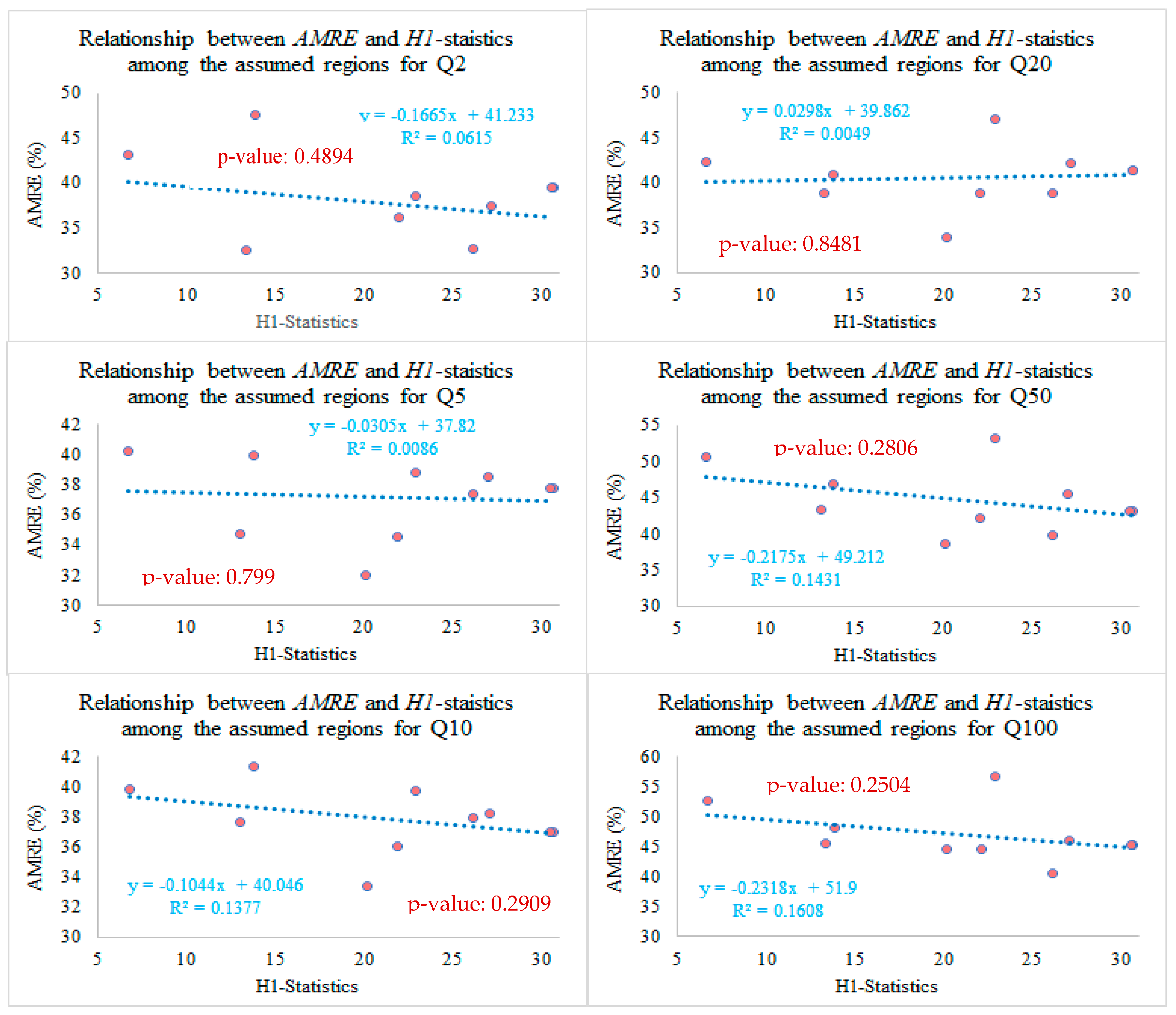
The scatter plot in Figure 8 illustrates the relationship between the heterogeneity level (measured by the H1-statistic) and AMRE values for the quantile estimates, with each dot representing an assumed region. The R2 values of the developed regression equations quantifies the degree of association between the H1-statistic and AMRE values of quantile estimation. The R2 values clearly indicate the weak relationship between the H1- and AMRE values associated with the regression equations. The maximum and minimum R2 values are 0.16 (p-value = 0.25) for Q100 and 0.005 (p-value = 0.85) for Q20, respectively. The trend/regression lines in Figure 8 (for all the six return periods) are not statistically significant (p-values range from 0.25 to 0.84), which indicates that the impact of the degree of heterogeneity on absolute median relative error is statistically insignificant. The minor inverse relationship or likely plateau conditions indicate no relationship between the degree of heterogeneity and the prediction accuracy of the developed regression equations. Figures S12–S15 (see Supplementary Section) also show the categorical spatial distribution of absolute RE values from Q20 quantile estimates for KNN50, KNN100, KNN150, and KNN200.
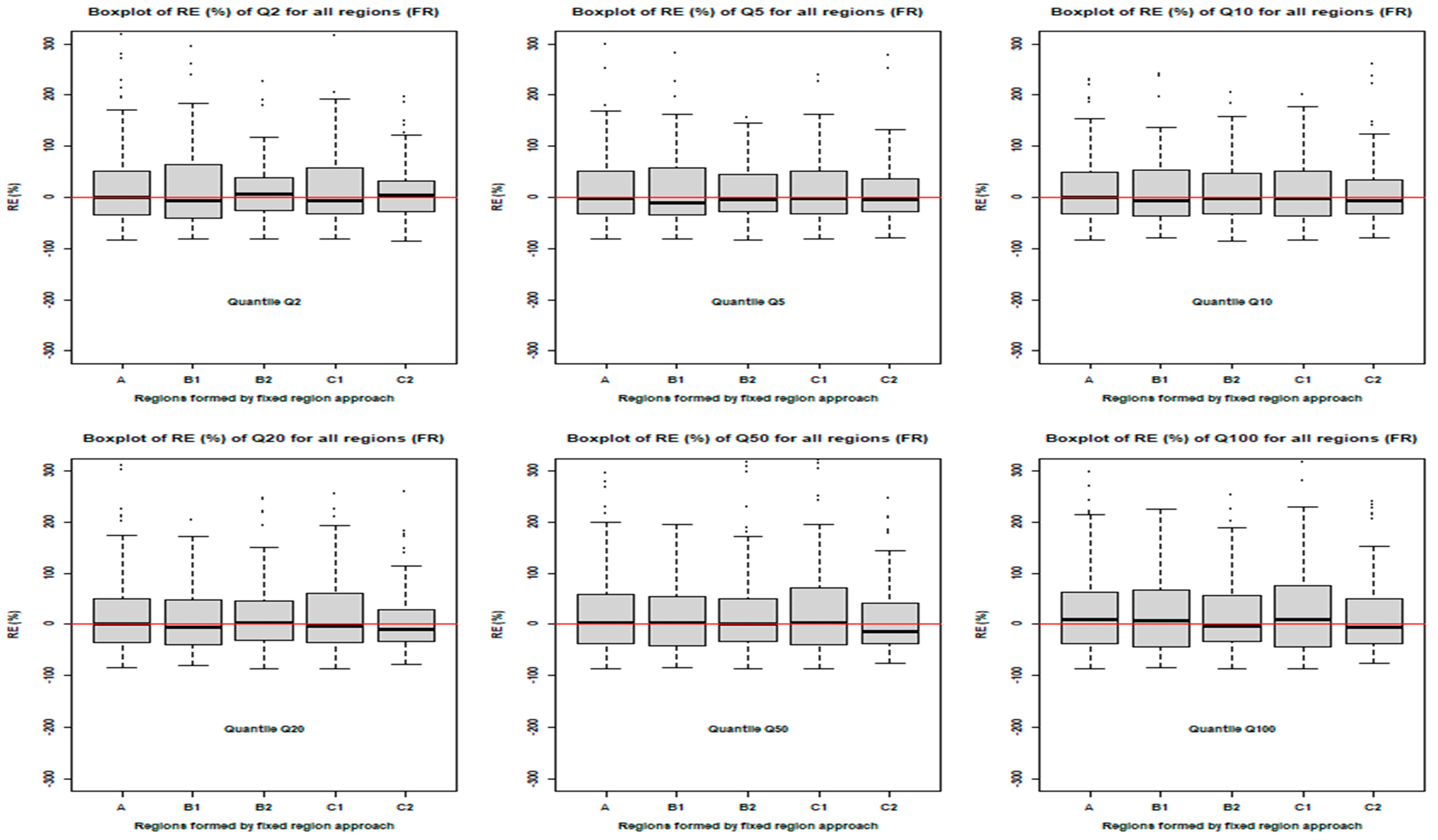
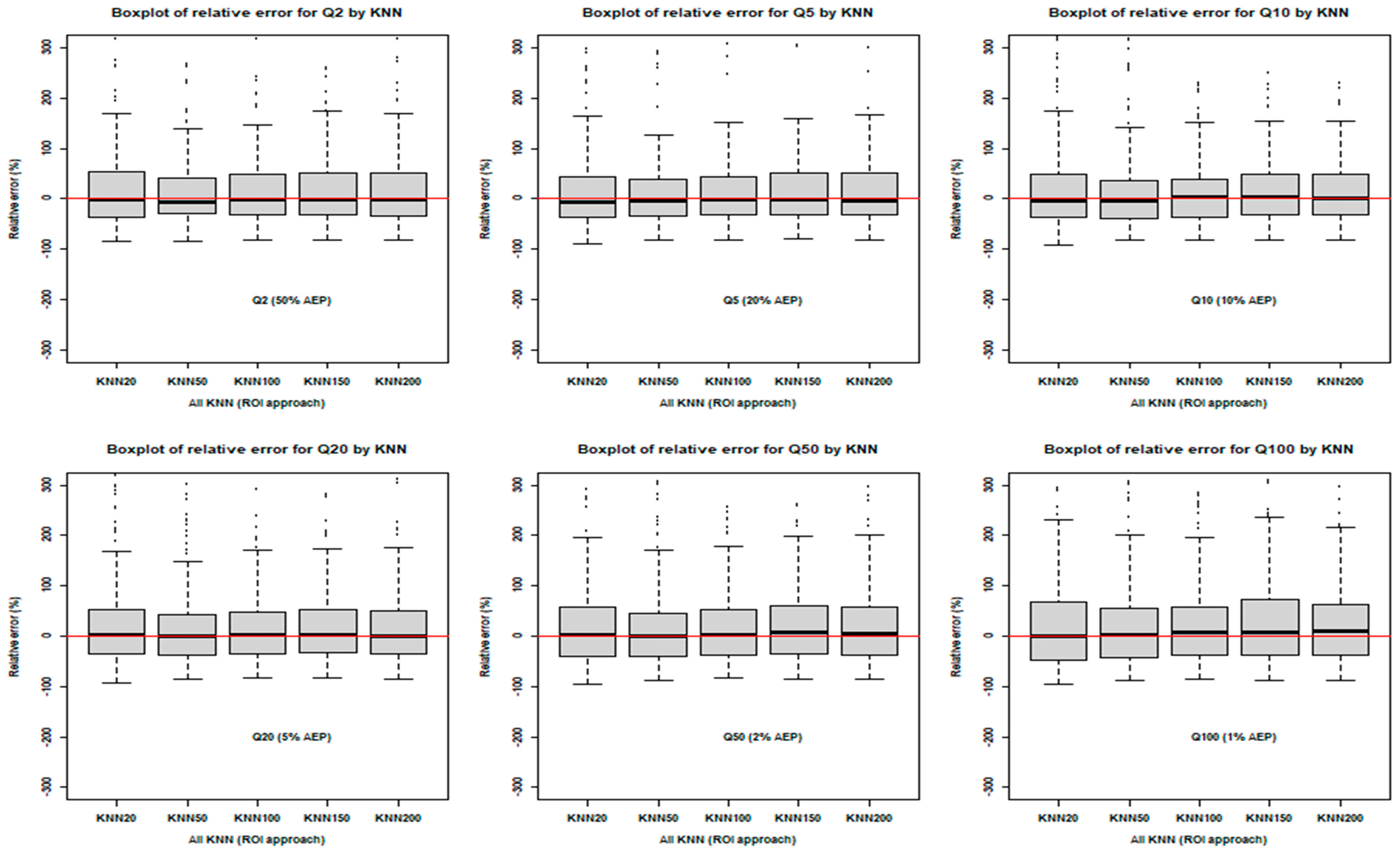
Figure 9 presents distribution of RE values by quantile estimates for all the assumed fixed regions. If the RE value of the prediction model is close to zero, then the model is called an unbiased model. In addition, for clearer visualization the boundary limit is set between −300 and 300, Figure 9 apparently indicates that the median RE value for most of the quantiles is generally close to the zero line for region B2. To some extent, the RE values for the regions A and C1 also touch the zero line. Having some under- and over-estimation, the regions A, B2, and C1 exhibit relatively precise RE estimates. Similar findings are also noticed in Figure 7 for the regions B2 (AMRE value < 41% for Q100) and A (AMRE value < 46% for Q100); however, surprisingly, in region C1 the AMRE value is high (ranges from 38.58% for Q2 to 56.66% for Q100). The fixed-region approach gives better quantile estimates for Q10, followed by Q5. In Figure 10, the ROI (KNN 20, 50, 100, 150, and 200) approach results in some under- and over-estimation of design flood estimates for the quantiles Q2, Q5, Q10, Q20, Q50, and Q100. However, the unbiased line (red line) roughly passes through the median values of RE of the Q20 quantile for all the KNNs compared to other quantiles. It also exhibits less variation in terms of RE values, which indicates that the ROI approach generates the best quantile estimates for the Q20 quantile. In the case of Q100, higher variation is observed (RE values deviate far away from the median RE values) compared to other quantiles (Figure 10).
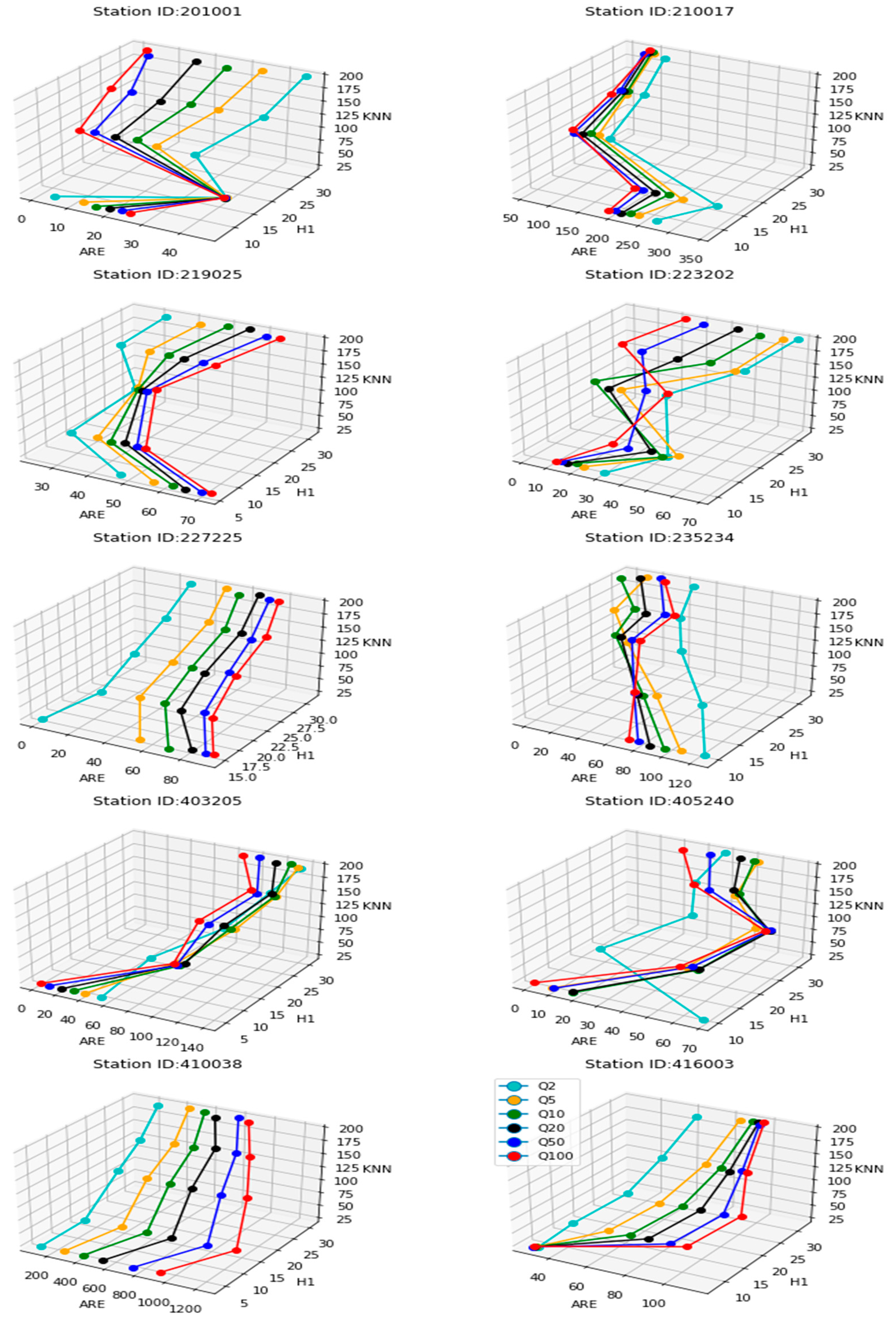
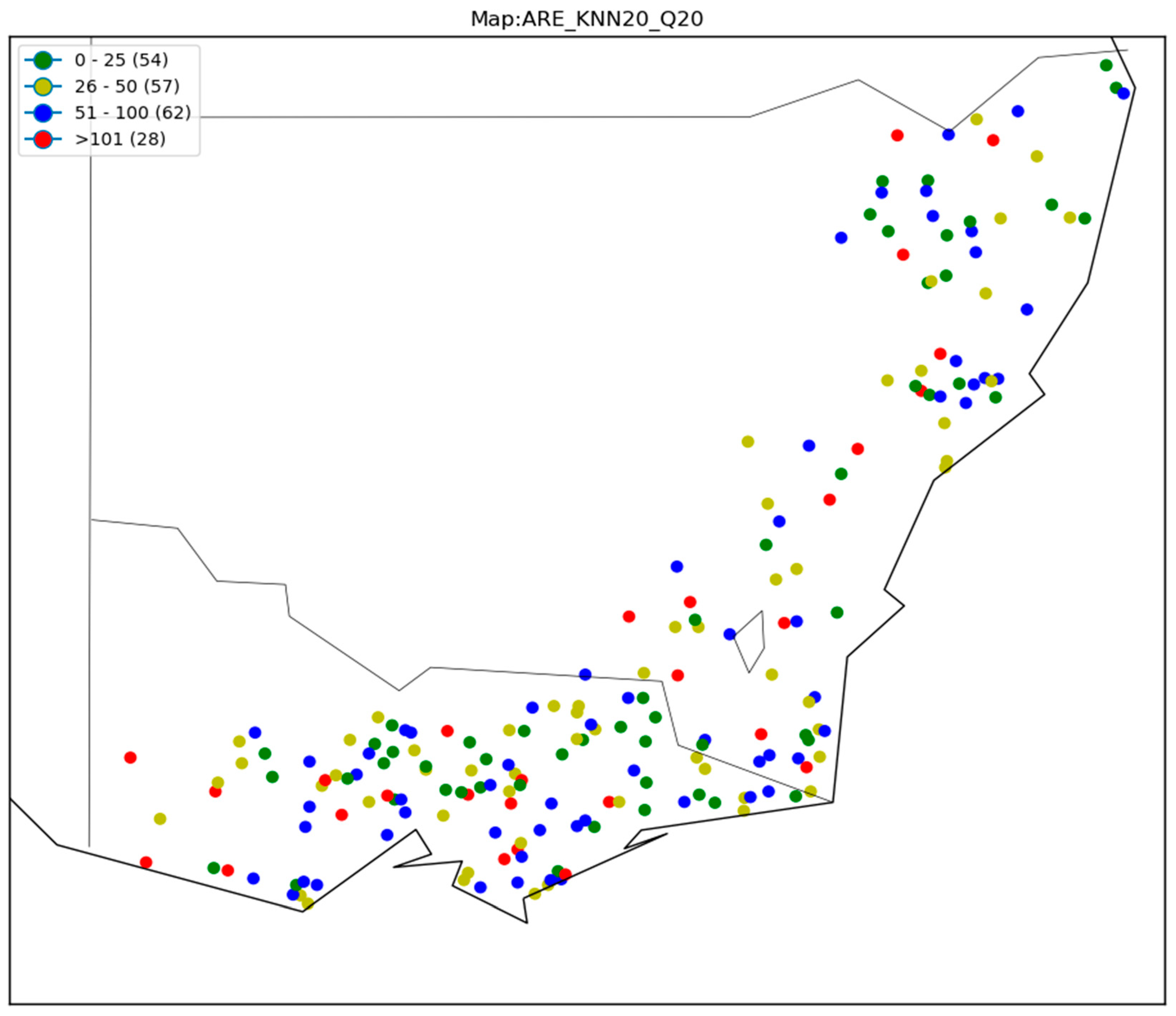
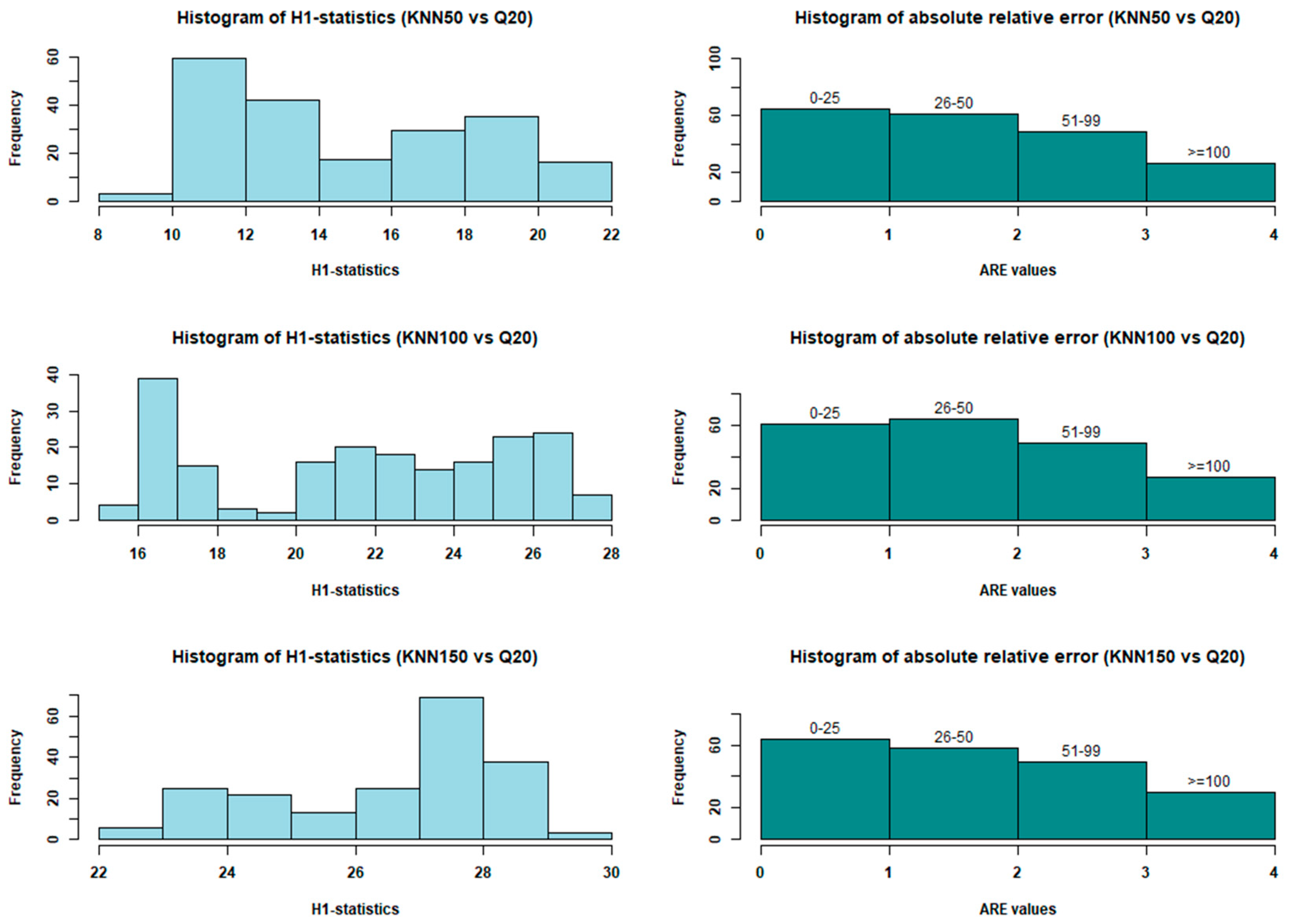
Based on Figure 9 and Figure 10, it can be said that the ROI approach outperforms the fixed-region approach by generating more precise flood quantile estimates for quantiles Q20 and Q5. Figure 11 shows a 3D visualization of the absolute RE and H1-values for the KNN regions. It explores the associations between the heterogeneity level and accuracy of quantile prediction. Figure 12 shows the categorical spatial distribution of AMRE values for Q20 for KNN20. Figure 13 (histogram) shows the comparison between H1-values and absolute RE values associated with Q20 for the KNN50, KNN100, and KNN150 regions. Similar plots can be found in Figures S5–S9 (Supplementary Section).
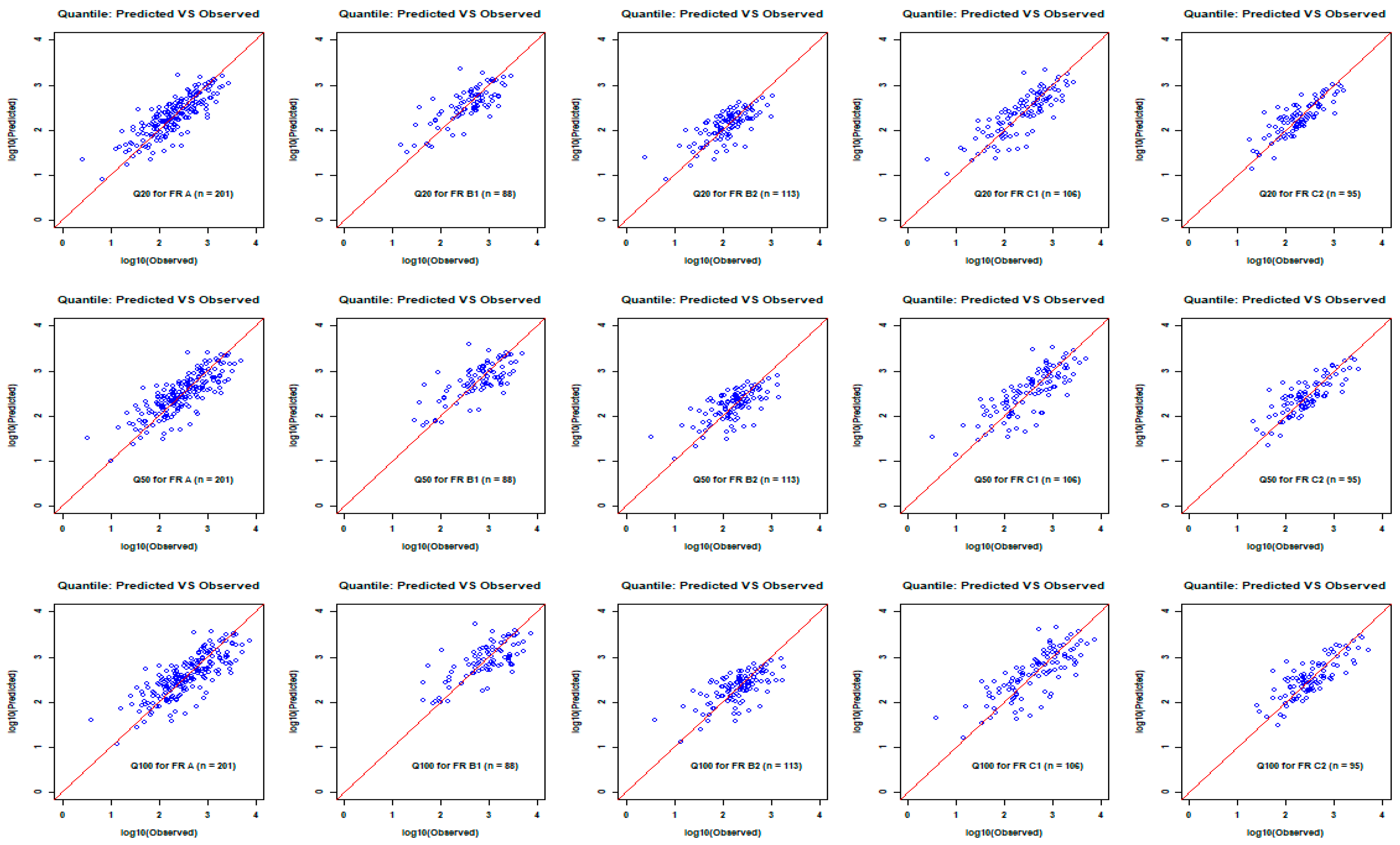
Figure 14 and Figure 15 explain the accuracy of quantile estimates through the scatter plots for the assumed regions (both the fixed-region and ROI approaches). The diagonal red line indicates the unbiased estimates. Log transformation ( l o g 10 ) is used to normalize the quantile values for better visualization. In both the figures, the 1st, 2nd, and 3rd row represent the scatter plots of quantile estimates Q20, Q50, and Q100, respectively, for different assumed regions. Figure 14 clearly indicates that the estimated quantile values are closer to the observed values in the C2 region. On the other hand, the observed and predicted values for the quantile are relatively closer to the unbiased line in regions KNN150 and KNN200 (Figure 15).

4. Discussion

The results of this study are compared with similar RFFA studies. Based on 305 stations in the USA, Basu and Srinivas [14] adopted a leave-one-out (LOO) validation technique to evaluate regional regression models under an ROI framework. The estimated absolute RBIAS values in this study ranged from 7.8 to 23.0 for Q50 and 12.8 to 33.4 for Q100. They also found that the RRMSE values in the range of 10.0% to 30.8% for Q50 and 16.2% to 44.3% for Q100 [14].
Using an ROI framework, based on 204 stream gauging stations in Arkansas, the defined unique subregion for each of selected stations showed an RMSE value of 38% [21]. Eng et al. [20] applied a hybrid ROI approach based on 1091 gauged stations in the southeastern USA for Q50. This hybrid ROI approach outperformed both the predictor variable and geographic-space-based ROI approach. The RMSE values from split-sample validation were in the range of 47.7–55.6%, 58.4–60.9%, and 50.3–56.2% for hybrid, predictor–variable and geographic-space-based ROI approaches, respectively [20]. Likewise, a multiple regression leverage-guided ROI approach was applied to 996 stations in the southeastern USA to estimate Q50. In case of geographic-space-based ROI, the estimated RMSE values reduced from 226% to 59%. On the other hand, the estimated RMSE values reduced to 22% from 48% and the variance of the leverage values decreased to 0.08 from 0.12 for predictor-based ROI [20].
Zrinji and Burn [13] conducted an RFFA study in mid-west Canada applying a hierarchical ROI approach. They found that the MSE values were in the range of 0.0654 to 0.0696, and the BIAS was in the range of −0.0109 to 0.0006 for different modelling options. Burn [17] conducted a study using 45 gauging stations in southern Manitoba, Canada to evaluate the ROI approach in terms of network average RMSE. The RMSE values ranged from 0.142 (Q25) to 0.298 (Q200). The estimated BIAS values ranged from 0.000 (Q25) to 0.023 (Q200). Durocher et al. [25] applied spatial copula on 151 gauging stations in southern Quebec, Canada. The estimated mean and median values of RMSE were 38 and 35, respectively, for Q10. These values were 45 and 41 for Q100, respectively [25]. Using the same dataset, several RFFA studies were conducted [26,27]. For these studies, the estimated RMSE values for Q10 ranged from 37 to 66 and from 45 to 86 for Q100. The estimated BIAS values ranged from −3% to −20% for Q10 and −2% to −27% for Q100.
In Australia, using a multiple liner regression-based RFFA approach with data from 88 stations in NSW, Rahman and Rahman [28] reported overall AMRE values ranging from 26.16% to 387.51%. Their H1-statistics ranged from 1.93 to 7.59, indicating the regions were heterogeneous. They also noticed a weak association between the degree of regional heterogeneity and the prediction accuracy of the developed regression equations [28]. In contrast, adopting independent component analysis and using the same dataset, Rahman et al. [29] found few discordant stations (Di values ranged from 3.78 to 6.05) and higher Hi-statistics (the H1, H2, and H3 statistics being 13.44, 10.06, and 5.96, respectively). Interestingly, they found less variation in AMRE values, which ranged from 33.28% (for Q20) to 43.92% (for Q2) for QRT. Using the parameter regression technique (PRT), AMRE values were found to be in the range of 47.84% (for Q5)–58.76% (for Q2). The reported MSE values ranged from 110,166 to 1,800,000. They found that the RBIAS and RRMSE values ranged from 22.04% to 68.93% and 0.00 to 0.27, respectively. The RMSNE values ranged from 0.95 to 3.60 [29]. However, using a global database (excluding Australia), Rosbjerg et al. [30] showed that the RMSNE values in a regression analysis are in the range of 0.50–0.65 [30].
In our study, the lowest and the highest Di values ranged from 3.05 to 7.18 (for the fixed regions) and 3.07 to 7.70 (for the ROI-based regions). The H1-statistics range from 13.83 to 30.66 for the fixed regions and from 6.71 to 30.57 for the ROIs. The overall median AMRE for quantile estimates is 40.00%. Though the H1-statistics are higher (potentially due to the highly variable Australian hydrology), in terms of Di and AMRE values, our study findings are similar to those of other Australian studies. The estimated overall median RBIAS among the assumed fixed regions in this study is 27.33; for ROIs it is 31.22. These figures for the RRMSE are 13% and 9%, respectively. These findings are comparable with the studies conducted in the USA, Canada, and Australia, as noted above.
To some extent, our AMRE, RBIAS, RMSE, and RRMSE values are more accurate than those of the few previous Australian studies, as noted above. Considering the estimated RMSNE values, the results of this study (0.70 to 2.25 for the fixed regions and 0.93 to 2.85 for the ROIs) appear to be more accurate compared to those from Rahman et al. [29] and less accurate than those of Rosbjerg et al. [30].
Our results show that southern and western Victoria (Figure 6) exhibit high levels of spatial heterogeneity, represented by shades ranging from light to deep red. In contrast, mid-northern Victoria demonstrates the highest degree of homogeneity, indicated by deep blue, with a similar though slightly reduced pattern observed in the southeastern corner of New South Wales. The underlying causes of these spatial variations remain poorly understood, and further investigation is required to clarify the hydrological processes driving this pattern.
It should be noted that the LCV and LCS of the AMF data are affected by data length; the length of data recording ranged from 25 to 89 years (a mean of 45 years). A shorter AMF data recording length, like 25 to 40 years (only around 14% of our stations have smaller recording lengths than 40 years), would have affected our results, e.g., H1-values. However, the impacts of a short recording length on our results are not explicitly addressed, except in the sub-division of the AMF data into three subsets: all data, AMF till 1990, and AMF from 1991 to 2018. The impacts of this data splitting are discussed in Section 3.3.

5. Conclusions

This study investigated the delineation of homogeneous regions for regional flood frequency analysis (RFFA) in southeast Australia using both fixed-region and region-of-influence (ROI) approaches. The relationship between regional heterogeneity and the predictive performance of regression-based RFFA models was also evaluated. Regions were delineated based on three fixed-region configurations: a single region encompassing all 201 stations and divisions based on either administrative state boundaries or drainage divisions. Additionally, a K-nearest neighbour (KNN) ROI method was employed to form flexible, site-specific regions. The degree of regional homogeneity was assessed using the statistical measures proposed by Hosking and Wallis [5].
Key findings from the study are as follows:
(i)
The Pearson Type III (PE3) and Generalized Pareto (GPA) distributions are identified as the most suitable probability distributions for RFFA in southeast Australia.
(ii)
The majority of the proposed regions exhibit high levels of heterogeneity. Although the KNN10 approach identifies 29 regions with acceptable homogeneity (H1 < 1.00), these regions include fewer than 20 sites each and are therefore considered too small to be statistically robust.
(iii)
The absolute median relative error (AMRE) values associated with the developed regression equations range from 29.50% for the 2-year return period (Q2) to 56.66% for the 100-year return period (Q100), with an overall median AMRE of 39.79%.
(iv)
The level of regional heterogeneity appears to have minimal influence on the accuracy of flood quantile predictions using regression-based methods in this region.
(v)
The ROI approach consistently outperforms the fixed-region approach in terms of predictive accuracy, particularly for the 20-year return period (Q20).
These findings highlight the limitations of conventional homogeneity-based regionalisation in highly diverse catchments and underscore the potential of ROI methods to provide more reliable flood estimates in such settings. Future research should explore the influence of climate change on both regional heterogeneity and the performance of regression-based RFFA. Additionally, there is a need to develop alternative homogeneity testing frameworks tailored for heterogeneous regions, particularly those applicable to regression-based methodologies.
Based on the findings of this study, it can be concluded with confidence that perfectly homogeneous regions for RFFA cannot be defined in southeast Australia. Therefore, engineers should avoid applying RFFA techniques that require strict regional homogeneity, such as the index-flood method. Instead, regression-based approaches are recommended for RFFA in southeast Australia, as they do not heavily rely on the homogeneity assumptions.

Supplementary Materials

The following supporting information can be downloaded at: https://www.mdpi.com/article/10.3390/w17182765/s1, Figure S1: Groups formed by cluster analysis (Ward’s method) (Stations are labelled by site index as per Table S1); Figure S2: Boxplots of LCV of AMF data for three assumed regions by cluster analysis (Ward’s Method, refer Figure S1); Figure S3: Spatial distribution of H1-statistics for KNN50 (ROI); Figure S4: Spatial distribution of H1-statistics for KNN100 (ROI); Figure S5: Comparison of H1-statistics and ARE values for Q2 for KNN50, KNN100 and KNN150; Figure S6: Comparison of H1-statistics and ARE values for Q5 for KNN50, KNN100 and KNN150; Figure S7: Comparison of H1-statistics and ARE values for Q10 for KNN50, KNN100 and KNN150; Figure S8: Comparison of H1-statistics and ARE values for Q50 for KNN50, KNN100, and KNN150; Figure S9: Comparison of H1-statistics and ARE values for Q100 for KNN50, KNN100 and KNN150; Figure S10: Spatial distribution of H1-statistics for KNN20 (ROI) for the sites having AMF data up to 1990; Figure S11: Spatial distribution of H1-statistics for KNN20 (ROI) for the sites having AMF data covering 1991 to 2018; Figure S12: Spatial distribution of ARE for Q20 of KNN50; Figure S13: Spatial distribution of ARE for Q20 of KNN100 Figure S14: Spatial distribution of ARE for Q20 of KNN150 Figure S15: Spatial distribution of ARE for Q20 of KNN200; Table S1: Selected catchments and their important characteristics; Table S2: Summary of identified homogeneous regions by ROI method (H1 < 1.00) with H1 values and their station IDs; Table S3: Regression coefficients for the developed models to estimate design floods for all assumed regions adopting fixed region and region-of-influence (ROI) approaches.

Author Contributions

Data analysis, investigation, and manuscript drafting: A.A.; investigation and editing: M.A.M.; methodology, investigation, and editing: S.T.M.; conceptualisation, investigation, and editing: R.S.M.H.R.; data analysis and editing: Z.K.; investigation and editing: R.M.; conceptualisation, editing, and supervision: A.R. All authors have read and agreed to the published version of the manuscript.

Funding

No funding was received by this research.

Data Availability Statement

The data used in this study can be obtained from Australian Government authorities by paying a prescribed fee.

Acknowledgments

The authors would like to acknowledge the Australian Rainfall and Runoff Revision Project 5 team for providing some of the data used in this study. TUFLOW FLIKE was provided freely by the FLIKE sales team. Streamflow data were obtained from WaterNSW, the entity of NSW state Government, Australia.

Conflicts of Interest

The authors state no conflicts of interest.

References

  1. Dalrymple, T. Flood-Frequency Analyses (No. 1543); Manual of Hydrology: Part 3; United States Government Printing Office: Washington, DC, USA, 1960.
  2. Shu, C.; Ouarda, T.B. Flood frequency analysis at ungauged sites using artificial neural networks in canonical correlation analysis physiographic space. Water Resour. Res. 2007, 43, 7. [Google Scholar] [CrossRef]
  3. Burn, D.H. An appraisal of the “region of influence” approach to flood frequency analysis. Hydrol. Sci. J. 1990, 35, 149–165. [Google Scholar] [CrossRef]
  4. Cunnane, C. Review of statistical models for flood frequency estimation. In Hydrologic Frequency Modelling; Springer: Dordrecht, The Netherlands, 1987; pp. 49–95. [Google Scholar]
  5. Hosking, J.R.M.; Wallis, J.R. Some statistics useful in regional frequency analysis. Water Resour. Res. 1993, 29, 271–281. [Google Scholar] [CrossRef]
  6. Stedinger, J.R.; Tasker, G.D. Regional hydrologic analysis: 1. Ordinary, weighted, and generalized least squares compared. Water Resour. Res. 1985, 21, 1421–1432. [Google Scholar] [CrossRef]
  7. Haddad, K.; Rahman, A. Regional flood frequency analysis in eastern Australia: Bayesian GLS regression-based methods within fixed region and ROI framework—Quantile Regression vs. Parameter Regression Technique. J. Hydrol. 2012, 430–431, 142–161. [Google Scholar] [CrossRef]
  8. Mediero, L.; Kjeldsen, T.; Macdonald, N.; Kohnova, S.; Merz, B.; Vorogushyn, S.; Wilson, D.; Alburquerque, T.; Blöschl, G.; Bogdanowicz, E. Identification of coherent flood regions across Europe by using the longest streamflow records. J. Hydrol. 2015, 528, 341–360. [Google Scholar] [CrossRef]
  9. Pinos, J.; Quesada-Román, A. Flood Risk-Related Research Trends in Latin America and the Caribbean. Water 2021, 14, 10. [Google Scholar] [CrossRef]
  10. Singh, A.K.; Chavan, S.R. An approach to regional flood frequency analysis for general peak discharge distribution datasets. J. Hydrol. 2025, 650, 132493. [Google Scholar] [CrossRef]
  11. Wiltshire, S.E. Grouping basins for regional flood frequency analysis. Hydrol. Sci. J. 1985, 30, 151–159. [Google Scholar] [CrossRef]
  12. Li, Z.; Gao, S.; Chen, M.; Gourley, J.J.; Hong, Y. Spatiotemporal characteristics of US floods: Current status and forecast under a future warmer climate. Earth’s Future 2022, 10, e2022EF002700. [Google Scholar] [CrossRef]
  13. Zrinji, Z.; Burn, D.H. Regional flood frequency with hierarchical region of influence. J. Water Resour. Plan. Manag. 1996, 122, 245–252. [Google Scholar] [CrossRef]
  14. Basu, B.; Srinivas, V.V. Regional flood frequency analysis using kernel-based fuzzy clustering approach. Water Resour. Res. 2014, 50, 3295–3316. [Google Scholar] [CrossRef]
  15. Ouarda, T.B.; Bâ, K.M.; Diaz-Delgado, C.; Cârsteanu, A.; Chokmani, K.; Gingras, H.; Quentin, E.; Trujillo, E.; Bobée, B. Intercomparison of regional flood frequency estimation methods at ungauged sites for a Mexican case study. J. Hydrol. 2008, 348, 40–58. [Google Scholar] [CrossRef]
  16. Durocher, M.; Burn, D.H.; Mostofi Zadeh, S. A nationwide regional flood frequency analysis at ungauged sites using ROI/GLS with copulas and super regions. J. Hydrol. 2018, 567, 191–202. [Google Scholar] [CrossRef]
  17. Burn, D.H. Evaluation of regional flood frequency analysis with a region of influence approach. Water Resour. Res. 1990, 26, 2257–2265. [Google Scholar] [CrossRef]
  18. Oudin, L.; Andréassian, V.; Perrin, C.; Michel, C.; Le Moine, N. Spatial proximity, physical similarity, regression and ungaged catchments: A comparison of regionalization approaches based on 913 French catchments. Water Resour. Res. 2008, 44, 3. [Google Scholar] [CrossRef]
  19. Merz, R.; Blöschl, G. Flood frequency regionalisation—Spatial proximity vs. catchment attributes. J. Hydrol. 2005, 302, 283–306. [Google Scholar] [CrossRef]
  20. Eng, K.; Milly, P.; Tasker, G.D. Flood regionalization: A hybrid geographic and predictor-variable region-of-influence regression method. J. Hydrol. Eng. 2007, 12, 585–591. [Google Scholar] [CrossRef]
  21. Tasker, G.D.; Hodge, S.A.; Barks, C.S. Region of Influence Regression for Estimating the 50-Year Flood At Ungaged Sites 1. JAWRA J. Am. Water Resour. Assoc. 1996, 32, 163–170. [Google Scholar] [CrossRef]
  22. Zhang, Z.; Stadnyk, T.A. Investigation of Attributes for Identifying Homogeneous Flood Regions for Regional Flood Frequency Analysis in Canada. Water 2020, 12, 2503. [Google Scholar] [CrossRef]
  23. Thomas, D.; Benson, M.A. Generalization of Streamflow Characteristics from Drainage-Basin Characteristics; US Government Printing Office: Washington, DC, USA, 1970.
  24. Kuczera, G.; Franks, S. At-site flood frequency analysis. In Australian rainfall & runoff; Ball, J., Babister, M., Nathan, R., Weeks, B., Weinmann, E., Retallick, M., Testoni, I., Coombers, P., Roso, S., Ward, M., et al., Eds.; Commonwealth of Australia: Symonston, Australia, 2019; Chapter 2, Book 3. [Google Scholar]
  25. Durocher, M.; Chebana, F.; Ouarda, T.B. On the prediction of extreme flood quantiles at ungauged locations with spatial copula. J. Hydrol. 2016, 533, 523–532. [Google Scholar] [CrossRef]
  26. Chebana, F.; Charron, C.; Ouarda, T.B.; Martel, B. Regional frequency analysis at ungauged sites with the generalized additive model. J. Hydrometeorol. 2014, 15, 2418–2428. [Google Scholar] [CrossRef]
  27. Wazneh, H.; Chebana, F.; Ouarda, T.B. Optimal depth-based regional frequency analysis. Hydrol. Earth Syst. Sci. 2013, 17, 2281–2296. [Google Scholar] [CrossRef]
  28. Rahman, A.S.; Rahman, A. Application of Principal Component Analysis and Cluster Analysis in Regional Flood Frequency Analysis: A Case Study in New South Wales, Australia. Water 2020, 12, 781. [Google Scholar] [CrossRef]
  29. Rahman, A.S.; Khan, Z.; Rahman, A. Application of independent component analysis in regional flood frequency analysis: Comparison between quantile regression and parameter regression techniques. J. Hydrol. 2020, 581, 124372. [Google Scholar] [CrossRef]
  30. Rosbjerg, D.; Bloschl, G.; Burn, D.; Castellarin, A.; Croke, B.; Di Baldassarre, G.; Iacobellis, V.; Kjeldsen, T.R.; Kuczera, G.; Merz, R. Prediction of floods in ungauged basins. In Runoff Prediction in Ungauged Basins: Synthesis Across Processes, Places and Scales; Cambridge University Press: Cambridge, UK, 2013; pp. 189–225. [Google Scholar]
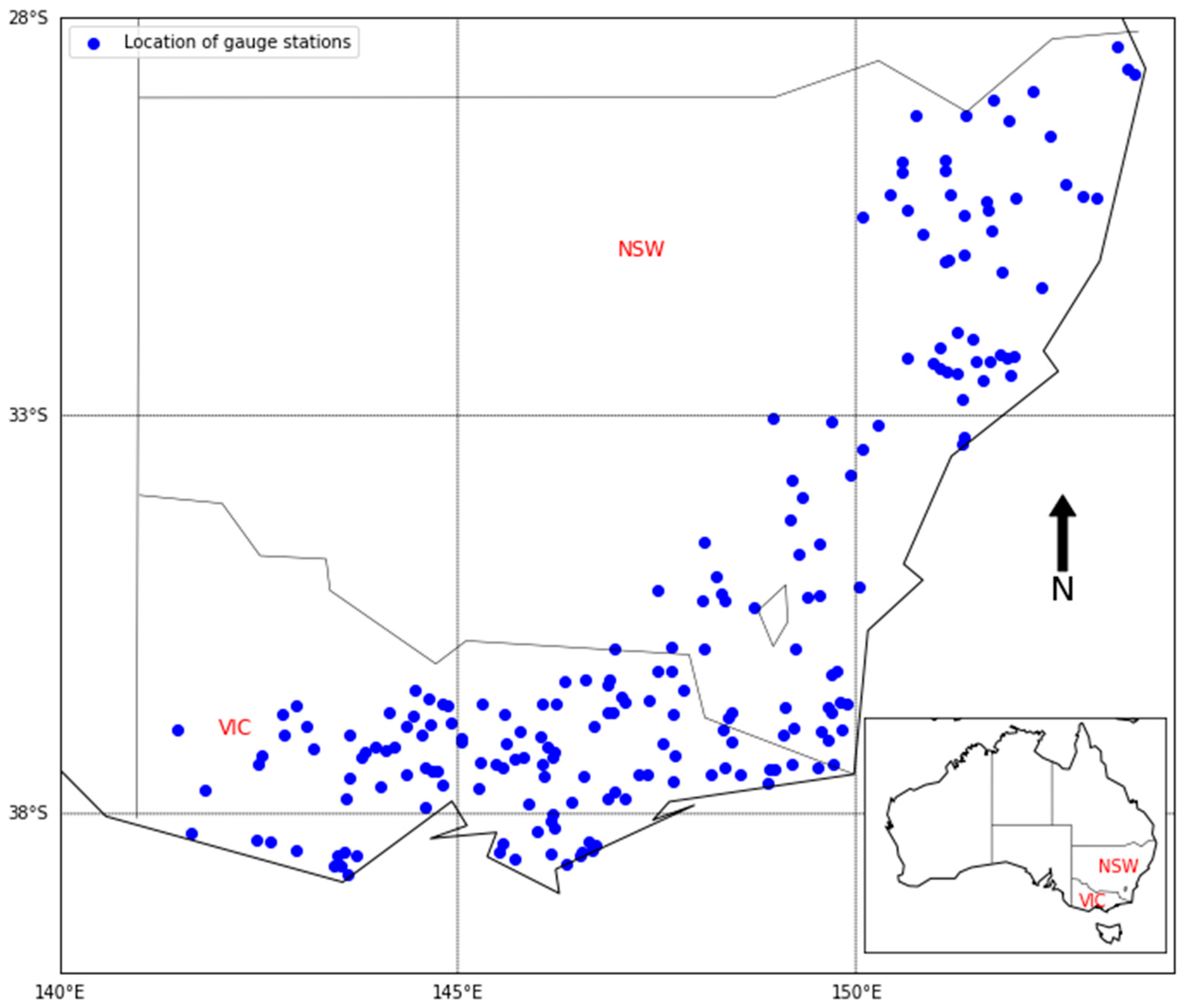
Figure 1. Spatial distribution of 201selected stations in southeast Australia.
Water 17 02765 g001
Figure 2. Boxplots of predictors and L-moments for the assumed regions.
Water 17 02765 g002
Figure 3. Comparison of Hi-statistics (median) among different candidate groups adopting fixed-region and ROI approaches.
Water 17 02765 g003
Figure 4. Pockets of identified homogeneous regions (red colour) for KNN10.
Water 17 02765 g004
Figure 5. Boxplots of H1-statistics for different regions (ROI approach). Red line refers threshold value for H1 = 1.00.
Water 17 02765 g005
Figure 6. Spatial distribution of H1-statistics for KNN20 (ROI).
Water 17 02765 g006
Figure 7. Comparison of absolute median relative error (AMRE) among the assumed regions, with H1-statistics.
Water 17 02765 g007
Figure 8. Scatter plots showing the association between H1- and AMRE values for the assumed fixed regions. Each dot refers the coordinates of H1- and AMRE-values. Red colors indicate the p-values and blue colors stand for fitted regression line with R2-values.
Water 17 02765 g008
Figure 9. Boxplots of relative error of the quantile estimates for the assumed fixed regions. The red lines indicate the estimated RE-values are set at zero (0), which means the predicted and observed quantile estimates are equal. Each dot refers to the RE-values for respective regions.
Water 17 02765 g009
Figure 10. Boxplots of relative error of the quantile estimates for the assumed regions adopting the ROI approach via KNNs. The red lines indicate the estimated RE-values are set at zero (0), which means the predicted and observed quantile estimates are equal. Each dot refers to the RE-values for respective regions (KNN).
Water 17 02765 g010
Figure 11. Three-dimensional plots of absolute relative error and H1-statistics among the assumed regions for randomly selected stations.
Water 17 02765 g011
Figure 12. Spatial distribution of AMRE for Q20 (KNN20).
Water 17 02765 g012
Figure 13. Comparison of H1-statistics and ARE values for Q20 (KNN50, KNN100, and KNN150).
Water 17 02765 g013
Figure 14. Scatter plots of observed and predicted quantiles in the assumed regions via the fixed-region approach. Each blue dot refers the coordinates of observed and predicted values of quantile estimates.
Water 17 02765 g014
Figure 15. Scatter plots of observed and predicted quantiles in the assumed regions via the ROI approach. Each blue dot refers the coordinates of observed and predicted values of quantile estimates.
Water 17 02765 g015
Table 1. Summary of descriptive statistics of the catchment characteristics (n = 201).
Station CharacteristicsMinimumMaximumMedianMeanStandard
Deviation
Catchment area (AREA, km2)3.001010.00261.00333.99262.40
Rainfall intensity (I62) (mm/h)24.6087.3037.3039.1610.07
Mean annual rainfall (MAR) (mm)484.391953.23891.64962.26314.47
Shape factor (SF)0.261.630.780.780.21
Mean annual evapotranspiration (MAE) (mm)925.901543.301076.701117.96129.31
Stream density (SDEN) (/km)0.525.471.692.101.06
Mainstream slope (S1085) (m/km)0.8069.909.5013.1911.67
Forest (FOREST) (fraction)0.001.000.590.550.34
Table 2. Summary of region formation (with notation), Di, Hi-, and Z-statistics for the assumed regions adopting fixed-region and ROI approaches.
Regionalization
Approach
Region
Notation
Number of Stations (n)Di-Values (≥3.00)Z-Statistics
LowestHighestGLOGEVGNOPE3GPA
Fixed-region approachA2013.266.4316.5512.497.27−1.77−0.04
B1883.055.439.827.734.06−2.280.65
B21133.095.0414.1510.386.650.16−0.49
C11063.345.3614.4111.127.110.151.12
C2953.057.189.697.083.53−2.61−1.09
Region-of-influence (ROI) approachKNN1010--3.933.001.79−0.340.07
KNN2020--5.274.192.33−0.750.18
KNN50503.075.538.296.383.64−1.030.35
KNN1001003.145.4011.558.734.90−1.52−0.76
KNN1501503.627.7014.3710.726.27−1.46−0.47
KNN2002003.266.4316.8212.707.42−1.740.01
Table 3. Regression coefficients associate with the predictor variables for Q50.
Region (No. of Sites)Regression CoefficientsAdj-R2
β0β1β2β3β4β5β6β7β8
ConsAREA
(km2)
I62
(mm/h)
MAR
(mm)
SFMAE
(mm)
SDEN
(/km)
S1085
(m/km)
FOREST
(Fraction)
A (201)−4.050.702.90−0.91−0.280.940.36−0.01−0.010.68
B1 (88)−1.240.733.10−0.91−0.55−0.130.400.07−0.030.62
B2 (113)−1.670.632.32−0.690.080.350.08−0.090.060.57
C1 (106)−5.000.733.30−0.87−0.401.000.080.070.000.70
C2 (95)−6.390.781.07−0.51−0.162.150.570.02−0.070.71
KNN20 (20)−4.190.812.07−0.88−0.431.650.190.10−0.120.81
KNN50 (50)−5.990.771.89−0.83−0.101.760.250.01−0.050.66
KNN100 (100)−2.360.623.33−1.180.160.390.50−0.100.010.60
KNN150 (150)−4.940.663.33−0.94−0.181.120.40−0.100.010.60
KNN200 (200)−4.050.702.90−0.91−0.280.940.36−0.01−0.010.68
Table 4. Summary of evaluation criteria for the assumed regions adopting the fixed-region ROI method.
Evaluation CriteriaQuantilesFixed RegionRegion-of-Influence (ROI) ApproachOverall Statistics
AB1B2C1C2KNN20KNN50KNN100KNN150KNN200StatisticsFRROI
R2Q20.720.730.710.800.690.840.740.690.700.72MIN0.530.58
Q50.730.730.680.790.730.840.710.660.680.73MAX0.800.84
Q100.720.700.640.770.730.830.690.630.660.72Mean0.690.70
Q200.700.670.610.740.720.820.680.620.630.70Median0.700.69
Q500.680.620.570.700.710.810.660.600.600.68SD0.060.08
Q1000.660.590.530.670.700.790.640.590.580.66Range0.270.26
AMREQ239.4947.6232.7438.5829.5043.1732.5336.1837.4739.49MIN29.5032.53
Q537.8039.9037.3838.8431.9340.2134.7734.5838.5037.80MAX56.6652.73
Q1036.9841.3937.9439.7833.3439.7937.6936.0738.2336.98Mean40.7240.85
Q2041.2540.9338.8047.0033.8142.3038.7238.7942.1241.25Median39.7240.00
Q5043.0446.9339.6653.1338.4850.6043.3842.1045.4143.04SD6.064.63
Q10045.3448.1240.5156.6644.6952.7345.5444.5146.0845.34Range27.1620.20
MSEQ2251548336133189101249262633267924762515MIN6132476
Q513,16727,029383618,573469534,69017,67116,73313,24013,167MAX1,576,1403,201,044
Q1036,47578,942954655,35712,713113,20955,25449,66637,08936,475Mean208,866353,981
Q2094,459209,80619,797147,94435,210333,229150,509130,18095,55594,459Median40,90295,007
Q50309,517686,27545,329480,016136,1891,247,541490,891410,848306,193309,517SD367,830641,000
Q100722,3281,576,14080,8561,087,259362,3603,201,0441,109,517915,078700,116722,328Range1,575,5283,198,568
BIASQ2−9.53−12.34−3.79−9.45−5.211.68−6.33−7.99−8.34−9.53MIN−233.05−169.16
Q5−20.05−24.10−10.20−18.50−11.364.82−10.69−13.63−14.22−20.05MAX−3.7993.24
Q10−33.25−40.63−17.61−31.20−20.149.93−15.48−20.44−21.66−33.25Mean−58.19−29.25
Q20−54.95−69.81−27.61−53.63−35.3120.36−23.68−31.83−34.90−54.95Median−34.28−20.25
Q50−105.43−140.90−46.05−108.35−71.6349.83−44.67−59.46−68.51−105.43SD58.9450.09
Q100−169.16−233.05−65.26−179.05−118.1093.24−73.51−95.85−113.74−169.16Range229.26262.40
RBIASQ222.2429.4116.8321.7716.4931.1024.7124.5427.9822.24MIN14.6321.41
Q521.4127.6019.6723.4414.6330.8826.4225.3326.5521.41MAX56.2068.05
Q1023.5531.1823.2127.7116.7835.1130.0028.1928.3723.55Mean29.0833.75
Q2026.9136.9027.0633.2820.0741.9634.4131.8731.3426.91Median27.3331.22
Q5032.7646.9332.5942.1825.6554.9641.1537.5836.4832.76SD10.2410.18
Q10038.1356.2037.1550.0130.6668.0546.8742.4541.1638.13Range41.5746.64
RRMSEQ20.150.130.100.120.110.030.100.130.130.15MIN0.100.03
Q50.130.100.110.100.100.030.070.090.090.13MAX0.210.21
Q100.130.100.130.100.100.040.060.080.090.13Mean0.140.10
Q200.150.120.150.120.120.050.060.090.090.15Median0.130.09
Q500.180.140.170.150.150.080.080.100.120.18SD0.030.04
Q1000.210.160.200.190.180.120.090.120.140.21Range0.110.18
RMSNEQ20.931.100.840.890.721.341.171.051.110.93MIN0.700.93
Q50.951.150.981.000.701.401.311.161.070.95MAX2.252.85
Q101.031.301.081.130.811.521.461.291.131.03Mean1.201.43
Q201.131.511.181.290.941.751.631.421.221.13Median1.141.35
Q501.291.891.321.521.142.261.871.611.361.29SD0.340.42
Q1001.422.251.431.721.312.852.071.761.471.42Range1.551.92
Standard deviation is used in the table to understand the variation of estimated evaluation criteria.
Disclaimer/Publisher’s Note: The statements, opinions and data contained in all publications are solely those of the individual author(s) and contributor(s) and not of MDPI and/or the editor(s). MDPI and/or the editor(s) disclaim responsibility for any injury to people or property resulting from any ideas, methods, instructions or products referred to in the content.