Article

A2DSC-Net: A Network Based on Multi-Branch Dilated and Dynamic Snake Convolutions for Water Body Extraction

1
College of Remote Sensing Information Engineering, North China Institute of Aerospace Engineering, Langfang 065000, China
2
Hebei Province Key Laboratory of Intelligent Processing of Remote Sensing Data and Target Analysis, Langfang 065000, China
3
Langfang Digital Space Technology Co., Ltd., Langfang 065000, China
4
Guangxi Xiande Environmental Protection Technology Co., Ltd., Nanning 530031, China
*
Author to whom correspondence should be addressed.
Water 2025, 17(18), 2760; https://doi.org/10.3390/w17182760
Submission received: 20 August 2025 / Revised: 12 September 2025 / Accepted: 16 September 2025 / Published: 18 September 2025

Abstract

The accurate and efficient acquisition of the spatiotemporal distribution of surface water is of vital importance for water resource utilization, flood monitoring, and environmental protection. However, deep learning models often suffer from two major limitations when applied to high-resolution remote sensing imagery: the loss of small water body features due to encoder scale differences, and reduced boundary accuracy for narrow water bodies in complex backgrounds. To address these challenges, we introduce the A2DSC-Net, which offers two key innovations. First, a multi-branch dilated convolution (MBDC) module is designed to capture contextual information across multiple spatial scales, thereby enhancing the recognition of small water bodies. Second, a Dynamic Snake Convolution module is introduced to adaptively extract local features and integrate global spatial cues, significantly improving the delineation accuracy of narrow water bodies under complex background conditions. Ablation and comparative experiments were conducted under identical settings using the LandCover.ai and Gaofen Image Dataset (GID). The results show that A2DSC-Net achieves an average precision of 96.34%, average recall of 96.19%, average IoU of 92.8%, and average F1-score of 96.26%, outperforming classical segmentation models such as U-Net, DeepLabv3+, DANet, and PSPNet. These findings demonstrate that A2DSC-Net provides an effective and reliable solution for water body extraction from high-resolution remote sensing imagery.

1. Introduction

Water resources are essential for the globe’s energy cycle, human activity, and the advancement of society. As an essential component of water resources, surface water exhibits pronounced spatiotemporal variability driven by both climate change and anthropogenic influences [1,2]. Consequently, surface water monitoring has long been a central focus of hydrology, environmental science, and remote sensing research. The extensive use of high-resolution imaging for water body extraction has been made possible by notable advancements in optical remote sensing sensor performance and resolution in recent years, with impressive outcomes. However, this task remains challenging due to the diverse morphological characteristics and complex spatial distribution of surface water, further compounded by the sensitivity of small-object extraction to environmental interference from surrounding features.

1.1. Conventional Water Index-Based Approaches

Water index-based approaches rely on the calculation of spectral ratios or differences between reflectance values across multiple bands to construct indices that effectively differentiate water from non-water surfaces. McFeeters proposed the Normalized Difference Water Index (NDWI), which can be effectively employed to extract water body information [3]. However, in urban environments, buildings and roads often exhibit spectral similarities to water, compromising NDWI performance for urban water extraction. To address these limitations, a variety of NDWI derivatives have been proposed, including the Modified Normalized Difference Water Index (MNDWI) [4], the Automated Water Extraction Index (AWEI) [5], and the Multi-Band Water Index (MBWI) [6]. In addition, numerous other indices have been developed in various studies to accommodate different sensors and regional conditions, each demonstrating varying degrees of accuracy [7,8,9,10]. This class of methods has low computational cost and does not rely on training data, allowing large-area images to be processed efficiently on commodity CPUs; it is thus well suited to rapid or near-real-time cartographic production. The main limitations lie in threshold sensitivity to scene context and a propensity to be confounded by shadows and intricate urban backgrounds. Nevertheless, under conditions of strong water-land spectral separation with minimal shadowing, or in data-poor and compute-limited settings, simple index approaches combined with adaptive thresholding (such as Otsu [11]) frequently deliver quicker and more stable performance, sometimes exceeding that of more sophisticated models.

1.2. Machine Learning-Based Methods

Machine learning-based methods typically leverage a combination of spectral bands and water-related indices as input features for model training. Fu et al. conducted a study in the Yellow River Delta, where they analyzed the spectral characteristics of water and various land cover types using TM imagery; they subsequently derived feature engineering rules based on spectral band combinations, including indices such as (Band4 − Band5)/(Band4 + Band5) and (Band3 − Band4)/(Band3 + Band4) [12]. Using a decision tree for iterative classification, Fu et al. achieved the automatic extraction of water bodies with high accuracy, particularly in the case of small-scale water features. Wang et al. proposed a rapid approach for estimating surface water dynamics by leveraging established water indices [13]. They computed the NDVI, NDWI, and MNDWI as part of the feature engineering process and subsequently applied a random forest classifier to extract water pixels. In comparison with water index-based methods, machine learning incorporates multi-source data, minimizing the dependence on a single global threshold, thus enhancing robustness in shadowed and urban environments. Compared to deep learning, these methods incur lower training and deployment costs, generally need fewer annotations, avoid GPU-based training, and can run efficiently on standard CPUs. Nevertheless, the performance of these methods is still contingent on feature design and regional parameterization; applying the model across different sensors or geographical areas often requires recalibration or further training.

1.3. Deep Learning Methods

Owing to its end-to-end learning paradigm, deep learning significantly minimizes manual intervention while autonomously learning hierarchical and multi-scale feature representations. This feature has made it easier for deep learning to be widely used in remote sensing image analyses, especially those involving the extraction of water bodies. An et al. introduced two key innovations, a reduced downsampling depth tailored to low-resolution imagery and a redesigned bottleneck structure optimized for encoder–decoder architectures [14]. Experimental results confirmed its strong practical utility. Guo et al. developed a semantic segmentation network incorporating dilated convolutions with varying dilation rates to capture water body features across multiple scales, achieving favorable performance on GF-1 imagery [15]. Wang et al. proposed a water extraction method based on a lightweight MobileNetV2 [16]. The experimental results showed that this method has high feasibility and segmentation accuracy. Li et al. investigated water body extraction from very-high-spatial resolution (VHR) optical imagery using a fully convolutional network (FCN) under limited training data conditions [17]. Through an empirical analysis involving 36 parameter configurations, they evaluated four critical factors influencing FCN performance: input features, training dataset size, transfer learning, and data augmentation. The insights gained from this work are transferable to the extraction of other land cover types. Building upon the U-Net architecture, Xu et al. proposed an information expansion network (IE-Unet). Experiments on a public water body dataset demonstrated its superior segmentation performance [18]. Li et al. proposed a method for extracting lake water bodies by fusing Sentinel-1/2 data, and achieved good extraction results for various types of lakes through support vector machine classification [19]. Sun et al. introduced WaterDeep [20], an enhanced deep learning framework with a novel feature fusion mechanism that integrates high- and low-level features. An experimental evaluation showed that WaterDeep outperforms existing deep learning models in water body extraction tasks. In another effort, MSFEN—a multi-scale feature extraction network—was developed for pixel-level surface water body extraction from medium-resolution remote sensing imagery [21]. By feeding the extracted features into traditional machine learning classifiers, MSFEN achieved superior performance compared to conventional fully convolutional networks.
Qi et al. proposed Dynamic Snake Convolution (DSConv) [22], which was initially applied to medical image segmentation. This convolutional operation adaptively concentrates on slender and tortuous local patterns, enabling the precise delineation of tubular structures. Its effectiveness has prompted its adoption in diverse fields. For instance, Qiao et al. developed DCP-Net for efficient forest fire segmentation, which accurately captures complex flame contours and significantly enhances intelligent fire detection capabilities [23]. In order to assist intelligent beef cattle detection and management systems, Li et al. introduced the YOLOv8n_BiF_DSC algorithm, which performs exceptionally well in feature extraction and high-level feature fusion [24]. Deep learning often delivers state-of-the-art accuracy in urban environments with narrow channels, intricate shorelines, and shadow coverage; however, it requires more labeled data and higher compute, and remains vulnerable to domain shifts across sensors, seasons, and geographic areas. Employing transfer learning, comprehensive data augmentation, and lightweight backbones can improve portability across domains [25]. When data and computational resources are limited or rapid mapping is needed, simple indices combined with adaptive thresholding provide better latency and engineering robustness [26]. Conversely, given sufficient annotations and computing, and in complex scenes, deep learning is the more appropriate choice for pursuing peak accuracy.

1.4. Persistent Challenges

Despite recent progress, several challenges remain in high-resolution water body extraction. First, significant variations in water body size may cause the encoder to lose critical feature information, thereby reducing accuracy [27]. Second, narrow water bodies occupy a relatively small proportion of images, with ambiguous boundaries and shapes, making them difficult to identify precisely. To address these issues, the main contributions of this study are summarized as follows:
  • Multi-branch dilated convolution module (MBDC): We design a multi-branch structure composed of dilated convolutions with different receptive fields to capture multi-scale contextual information, thereby improving the extraction of small water bodies.
  • Dynamic snake convolution with double attention mechanism: We introduce and adapt dynamic snake convolution to the water body extraction task for the first time. By enabling convolution kernels to adjust their shape and orientation adaptively, and combining them with a double attention mechanism, the model is able to better identify and represent complex water body structures.

2. Materials and Methods

2.1. Data Sources

Gaofen Image Dataset (GID) dataset: The GID dataset, derived from GF-2 satellite imagery, consists of two parts, the Fine Land Cover Classification Set (FLCCS) and the Large-Scale Classification Set (LSCS) [28]. The LSCS contains 150 GF-2 images, initially divided into five categories. We reclassified into two categories: water bodies and non-water bodies. After cropping into 512 × 512 pixel blocks and discarding blocks without water bodies, 9031 training, 1004 validation, and 2509 test samples were obtained.
LandCover.ai dataset: LandCover.ai [29] contains high-resolution aerial images, covering about 216 km2. After cropping into 512 × 512 pixel blocks and removing those without water bodies, the dataset yielded 7020 training, 781 validation, and 1951 test samples.
As shown in Figure 1, the datasets contain various types of water bodies. This demonstrates that the datasets can provide high-quality data support for this study.

2.2. Methods

2.2.1. A2DSC-Net Architecture

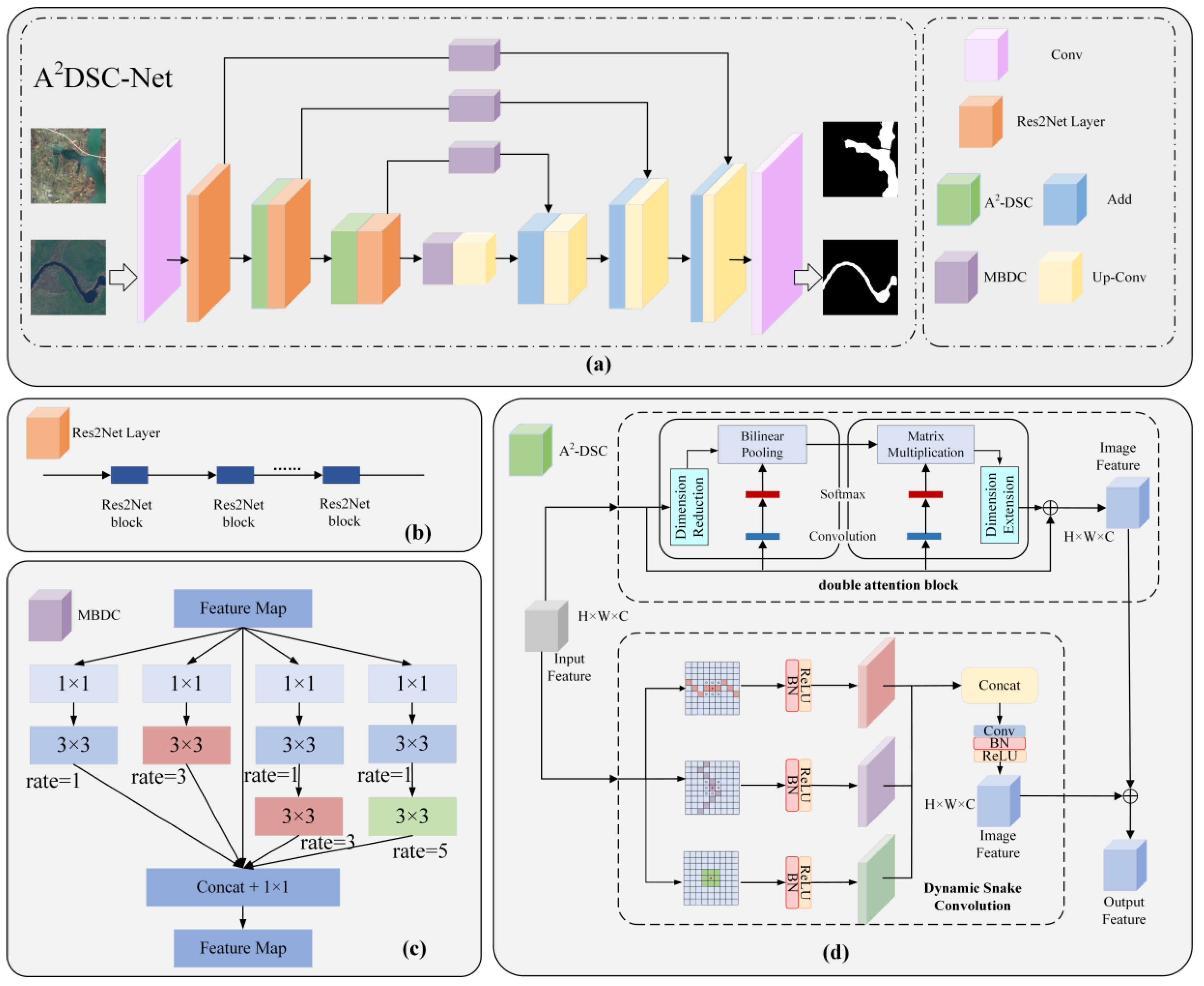
The A2DSC-Net architecture proposed in this study is illustrated in Figure 2a, and it consists of a multi-scale feature encoding part, a decoder, and a multi-scale feature extraction module. As the number of convolutional layers in the encoder increases, image information tends to be lost. To enhance feature extraction capability, Res2Net [30] is employed as the multi-scale feature encoder. As shown in Figure 2b, Res2Net expresses multi-scale features at a finer granularity and enlarges the receptive field of each layer. Specifically, for a feature map of 256 × 256 pixels, downsampling is performed at scales of {1/2, 1/4, 1/8}. With progressive downsampling, the spatial resolution of the feature maps decreases, allowing the extraction of high-level multi-scale water body features. Similarly, four convolution blocks are used in the decoder’s design to progressively recover high-resolution and high-quality feature representations. The feature map size is gradually upsampled using bilinear interpolation with a scaling factor of 2.
In deep learning models, pooling operations and strided convolutions are commonly used to reduce feature-map dimensions and expand the receptive field. However, these operations inevitably lead to information loss. To alleviate this issue, the A2DSC-Net integrates an MBDC module, which preserves edge information to the greatest extent possible, providing richer and more precise feature representations.

2.2.2. Multi-Branch Dilated Convolution (MBDC) Module

To capture contextual information at multiple scales and reduce the bad gridding issue [31], we designed the MBDC module to strengthen the network’s representation of water body features. This module employs a multi-branch architecture composed of dilated convolutions with varying kernel sizes. In addition to the standard convolutional parameters, dilated convolutions introduce an extra hyperparameter known as the dilation rate. By adjusting the dilation rate, one can seamlessly incorporate receptive fields of different sizes without increasing the number of kernel parameters. Figure 3 illustrates several 3 × 3 dilated convolutions with different dilation rates. A dilated convolution with rate d can be regarded as a standard convolution, where ( d 1 ) zeros are inserted between each row and column of the kernel. The calculation formula of the receptive field of the n t h layer of CNN r n is as follows [27]:
r n = r n 1 + K n 1 i = 1 n 1 S i
where K n denotes the kernel size of the n t h layer of the CNN, and S i denotes the stride of the i t h layer of the CNN.
As shown in Figure 2c, the MBDC module first applies a 1 × 1 convolution to the input features to reduce the channel count, and then it uses convolutional layers with varying kernel sizes and dilation rates to extract feature representations with diverse receptive fields. Finally, the outputs of all branches are concatenated and fused with the original feature map via a 1 × 1 convolution. Specifically, the first branch applies a 3 × 3 convolution with a dilation rate of 1 to capture the fine-grained context, the final branch stacks 3 × 3 convolutions with dilation rates of 1 and 5 to obtain the coarse-grained context, and the intermediate branches extract medium-scale semantic features; the semantic outputs of all five branches are then integrated.

2.2.3. Dynamic Snake Convolution Module

As high-resolution remote sensing images have finer granularity, their background environments have become more complex and diverse; as a result, water body features are more susceptible to interference and are affected by the complex background in the extraction process. We suggest the A2-DSC module, whose structure is depicted in Figure 2d, to significantly enhance the model’s capacity to identify subtle features. This module combines the features of DSConv [22] and a double attention block [32]. DSConv enhances the model’s ability to capture fine details of narrow water bodies, which are often difficult to detect with standard convolutional layers. The double attention block further refines feature representation by allowing global and local features to complement one another. This interaction enables the model to capture more intricate relationships between spatially distant features and improves the model’s robustness against background interference.
The fixed-shape convolution kernel used in the conventional 2D convolution procedure may make it more difficult for the model to concentrate on small, narrow water bodies. In contrast, DSConv can flexibly adapt its kernel shape, thereby effectively capturing the features of slender water bodies. The detailed implementation of DSConv is described below.
DSConv employs an iterative strategy that sequentially selects regions of interest for each object, thereby ensuring continuous attention. When the kernel size is 9, each position along the x-axis is denoted as K i ± c = ( x i ± c , y i ± c ) , where c = { 0,1 , 2,3 , 4 } represents the distance from the central cell. The selection of each position K i ± c within kernel K follows an accumulative process. Starting from the central position K i , each successive position depends on the previous one, where   K i is determined by its preceding position K i 1 plus an offset = { δ | δ [ 1,1 ] } . Accumulating these offsets ensures that the final convolutional kernel aligns linearly along the x-axis, mirroring the morphological traits of water bodies. The x-axis direction can be calculated as
K i ± c = x i + c , y i + c = x i + c , y i + i i + c y x i c , y i c = x i c , y i + i c i y
The y-axis direction can be calculated as
K j ± c = x j + c , y j + c = x j + j j + c x , y j + c x j c , y j c = x j + j c j x , y j c
The offset is generally fractional, and bilinear interpolation is used to yield more precise pixel values.
K = K B K , K K
where K denotes the decimal position in Equations (2) and (3); K ' denotes the spatial position of the integers; and B denotes the bilinear interpolation kernel, which is decomposed into two one-dimensional kernels, as follows:
B K , K = b K x , K x b K y , K y
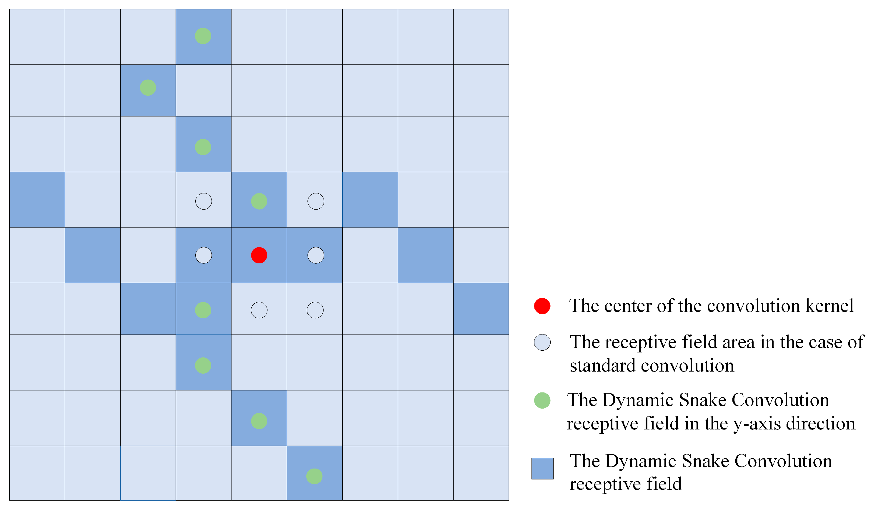
After the two-dimensional transformation, the DSConv receptive field appears as illustrated in Figure 4. This configuration more effectively conforms to the morphological characteristics of narrow, elongated water bodies, thereby laying the groundwork for precise water body extraction.
The double attention module operates in two stages—feature aggregation and feature distribution. Its design is inspired by SENet [33]. In SENet, the squeeze phase employs global average pooling to produce a single global descriptor, which is then uniformly applied across all spatial locations, overlooking the distinct requirements of individual positions. Consequently, the double attention module first gathers the global context via second-order attention pooling, and then it adaptively distributes this information according to local feature requirements through a secondary attention mechanism. In this manner, each spatial position receives a complementary global context that enriches its local features, thereby facilitating the capture of more intricate interdependencies.
Z i = F d i s t r G g a t h e r X , v i
where X R c × h × w denotes the input tensor; here, c is the number of channels, and h and w represent its height and width, respectively. First, features are aggregated across the entire spatial domain and then distributed to each input location i while also accounting for the local feature V i at that position. Specifically, G g a t h e r adaptively aggregates features across the entire input space, while F d i s t r distributes the collected information to each location i based on its local feature V i .
By introducing bilinear pooling, the feature aggregation component can be calculated as
G b i l i n e a r A , B = A B T
where A and B may originate from the same layer, i.e., A = B , or from different layers, denoted as A = ( X ; W ) and B = θ ( X ; W θ ) , with learnable parameters W and W θ . Specifically, A = a 1 , a 2 , . . . , a h w R m × h w , and B = b 1 , b 2 , . . . , b h w R n × hw . We then reshape B as B = b ¯ 1 ; b ¯ 2 ; . . . ; b ¯ n , where each b ¯ i is an h w -dimensional row vector. The resulting output is G = g 1 , g 2 , . . . , g n R m × n .
g i = A s o f t m a x b ¯ i T
After collecting features from the entire space, the next step is to distribute them to each position in the input, which can be calculated as follows:
z i = j V i j g j = G g a t h e r X V i ,   w h e r e   j V i j = 1
where V = s o f t m a x ρ X ; W ρ ; here, W ρ denotes the learnable parameters. By integrating the aforementioned feature aggregation and feature distribution steps, the double attention module is constructed.
Z = F d i s t r G g a t h e r X , V = G g a t h e r X s o f t m a x ρ X ; W ρ = X ; W s o f t m a x θ X ; W θ T s o f t m a x ρ X ; W ρ

2.3. Accuracy Assessment

This study can be viewed as a binary classification problem. Based on the true class and the model’s predicted class, four categories can be defined: true positive ( T P ), which indicates that the actual class is water, and the model also predicts it as water; false negative ( F N ), which indicates that the actual class is water, but the model predicts it as non-water; false positive ( F P ), which indicates that the actual class is non-water, but the model predicts it as water; and true negative ( T N ), which indicates that the actual class is non-water, and the model predicts it as non-water. To quantitatively assess the model’s effectiveness, precision, recall, Intersection over Union ( I o U ), and F 1 s c o r e are selected as evaluation metrics.
P r e c i s i o n = T P T P + F P
R e c a l l = T P T P + F N
I o U = T P T P + F N + F P
F 1 s c o r e = 2 × P r e c i s i o n × R e c a l l P r e c i s i o n + R e c a l l
where the precision rate represents the model’s prediction accuracy for positive samples, the recall rate refers to the proportion of samples predicted as true to all true positive samples, and the F 1 s c o r e is the reconciled average of the precision and recall rates, synthesizing the performance of the two. The I o U is an important metric for measuring model performance, as it evaluates the degree of overlap between predicted regions and ground truth regions.

3. Results

3.1. Ablation Experiments

In this section, we assess the performance of the MBDC and A2-DSC modules in the water body extraction task. To comprehensively and accurately assess the impact of these two modules, we carefully designed four different network models based on A2DSC-Net. First, we established a baseline network that does not include either the MBDC or A2-DSC module, serving as a reference point to observe performance changes as new modules are incrementally added. Next, the Baseline-MBDC model was created by incorporating the MBDC module into the baseline network. Subsequently, the A2-DSC module was added to the baseline, forming the Baseline-A2DSC model. All three variants, along with the proposed A2DSC-Net, were trained using identical hyperparameters, training protocols, and dataset splits. This rigorous experimental design enabled an accurate and objective evaluation of the effectiveness of the MBDC and A2-DSC modules.
  • Ablation Study of the MBDC Module
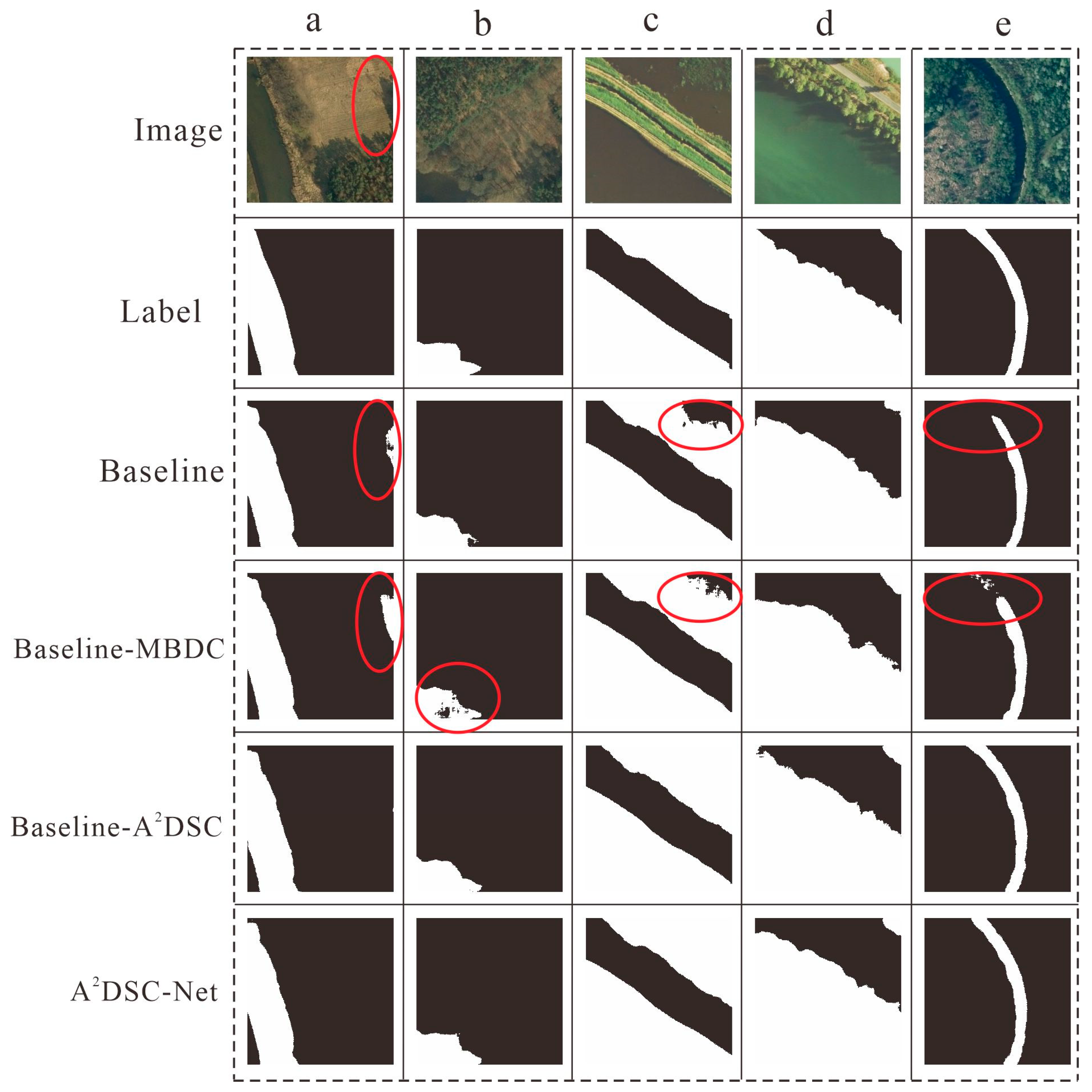
Compared to the baseline, Baseline-MBDC achieves improvements in recall, IoU, and F1-score of 0.47%, 0.03%, and 0.02% on the GID dataset and of 1.03%, 0.72%, and 0.39% on the LandCover.ai dataset, as shown in Table 1 and Table 2. For an intuitive comparison, Figure 5 and Figure 6 show several representative water body extraction results. In Figure 5b, both the Baseline-MBDC and baseline models exhibit clear shortcomings when dealing with narrow, winding water bodies, resulting in varying degrees of omission and incomplete extraction. Although the MBDC module brings some improvement, it still cannot overcome the challenges posed by the morphology of slender and curved water bodies. Figure 5e illustrates a scenario where clouds obscure water bodies; here, Baseline-MBDC outperforms the baseline, as the MBDC module better captures multi-scale image information and partially mitigates cloud interference. Both models are unable to discern between river bodies and tree shadows in Figure 6a, indicating that the MBDC module still lacks useful techniques for separating visually identical land cover types. The MBDC module can utilize contextual features from surrounding regions to further enhance the model’s water body extraction capabilities, but its performance remains limited when used alone, indicating the need for further investigation.
2.
Ablation Study of the A2-DSC Module
According to Table 1 and Table 2, the Baseline-A2DSC model achieves a 0.6% improvement in recall on the GID dataset, and it shows notable gains of 2.29%, 1.65%, and 0.89% in recall, IoU, and F1-score, respectively, on the LandCover.ai dataset when compared with the baseline model. As shown in Figure 5 and Figure 6, in Figure 5a, the baseline model cannot accurately detect a single small water body, whereas the Baseline-A2DSC model exhibits superior performance on such localized extraction tasks. The A2-DSC module performs particularly well in Figure 5b, precisely conforming to the contours of slender, sinuous water bodies and capturing their complex shape information. Compared with the baseline model, incorporating the A2-DSC module significantly improves the extraction of narrow water bodies. In Figure 6a, the baseline model struggles to distinguish between visually similar tree shadows and water bodies, whereas the Baseline-A2DSC network, benefiting from its optimized architecture, effectively separates the two, showcasing enhanced robustness in complex scenarios. Figure 6c reveals how vegetation intrusion affects water body recognition. The baseline model suffers from misclassification, whereas the Baseline-A2DSC network successfully suppresses vegetation interference and accurately delineates the true water extent. Figure 6e highlights the effectiveness of the A2-DSC module in extracting irregularly shaped, meandering water bodies. The module enables the model to produce complete and highly accurate representations that closely align with the actual morphology. According to the above results, the proposed A2DSC-Net demonstrates superior performance across both the GID and LandCover.ai datasets. The network effectively combines the complementary advantages of the MBDC and A2-DSC modules. By leveraging multi-branch structures and varied dilation rates, the MBDC module captures multi-scale contextual cues, supplying rich feature representations for precise water body segmentation. The A2-DSC module dynamically adapts kernel shapes to water body contours, significantly improving the model’s flexibility and morphological adaptability. Their integration empowers the network with exceptional capabilities in extracting complex and diverse water body forms.
Although the improvements in the ablation study are relatively modest, the A2DSC-Net integrates several novel modules that have not been combined in other methods. By incorporating these components, A2DSC-Net offers more robust performance across multiple tasks, particularly when dealing with complex backgrounds and high-resolution remote sensing images. The integration of these multi-modular components enhances the model’s flexibility and generalization ability. Moreover, we believe that even small improvements are highly significant in specific tasks and scenarios. For instance, in cases involving water body edges or narrow water bodies, A2DSC-Net provides more precise feature extraction and greater robustness, enabling the model to capture finer details and mitigate noise interference. This capability is crucial for certain remote sensing tasks.

3.2. Comparative Experiments

This study used representative models from the field, such as U-Net, PSPNet, DeepLabv3+, and DANet, as controls in a series of comparative experiments to assess the performance of the A2DSC-Net model in water body extraction. To ensure fairness in the comparative experiments, we strictly controlled the experimental conditions and used identical hyperparameters for all compared models, thereby eliminating the influence of parameter differences on model performance. We employed a unified loss function for all models to ensure that the training process was driven by the same optimization target. The same training, testing, and validation datasets were used to ensure that the model evaluation was conducted with consistent data distributions.

3.2.1. Comparative Experiments on the GID Dataset

Five scenarios were selected for presentation in Figure 7 to examine how well different networks extracted water bodies from the GID dataset. Specifically, in Figure 7a, PSPNet and DANet were almost unable to identify the presence of narrow and small water bodies. It is possible that neither network is capable of capturing features of tiny targets, resulting in the incomplete extraction of narrow water bodies. While DeepLabv3+ succeeded in identifying water bodies, the segmentation of their boundaries was rough and imprecise, likely because DeepLabv3+ has a limited capacity to handle fine-grained details in high-resolution imagery. By comparison, U-Net and A2DSC-Net performed well in this scenario, accurately identifying small, narrow water bodies and producing more refined boundary segmentation.
In Figure 7b, U-Net, PSPNet, and DANet all struggled with extracting curved, small water bodies. While the U-Net could partially recognize water bodies with irregular shapes, it could not precisely follow their contours. PSPNet and DANet had difficulty in capturing the complex morphology of water bodies, resulting in a large number of missed classifications. DeepLabv3+ and A2DSC-Net exhibited outstanding performance. DeepLabv3+ was able to grasp the global structure of sinuous small water bodies, enabling more precise extraction. A2DSC-Net can not only accurately identify the location of small winding water bodies but also precisely segment their complex boundaries, producing results highly consistent with the actual water bodies.
For the shallow and narrow water bodies in Figure 7c, PSPNet and DANet exhibited fragmentation, generating discontinuous short line segments instead of coherent water regions. DeepLabv3+ and U-Net’s extraction results are similarly inadequate, as several water bodies were overlooked during detection. Among all methods, only A2DSC-Net delivered promising results, deeply exploring the characteristics of shallow, narrow water bodies and accurately recognizing their spatial distribution with highly complete and accurate segmentation and minimal omission or error.
For the meandering water bodies in Figure 7d, most models achieved satisfactory extraction results, but there were still some problems in terms of detail. Except for DeepLabv3+, which exhibited imprecise and coarse boundary segmentation, U-Net, PSPNet, DANet, and A2DSC-Net performed approximate segmentation and correctly identified the general shape of the winding water bodies. However, when focusing on the small water body in the upper right corner of the image, DeepLabv3+ and U-Net exhibited misclassification issues. DeepLabv3+ may have misjudged the local features, mistakenly identifying the small water body as background or another land cover type. The classification error of the U-Net might stem from its limited ability to extract adequate feature information near image edges. In contrast, PSPNet, DANet, and A2DSC-Net achieved a relatively accurate identification of the small water body in this scenario, without significant misclassification. This indicates that these networks exhibit stronger robustness and accuracy when dealing with small targets in complex scenes.
In Figure 7e, all models were able to effectively identify the non-water areas within large water bodies. However, DeepLabv3+ and DANet exhibited substantial omission errors when extracting the internal regions of large water bodies. Some water body regions may have been unintentionally eliminated as a result of these two networks’ inadequate attention to internal detail features when processing large, homogeneous areas. PSPNet showed insensitivity to both boundaries and non-water areas; its results showed blurred edges and unclear separation between water and non-water regions, which compromised the overall extraction accuracy. U-Net and A2DSC-Net once again demonstrated superior performance in this scenario, extracting large water body features with higher precision and more accurately identifying internal non-water regions, achieving the best results among all models.
Table 3 presents the quantitative results obtained from comparing the five methods. Specifically, compared to DeepLabv3+, the A2DSC-Net model achieved increases of 3.11%, 0.96%, 3.67%, and 2.04% in precision, recall, IoU, and F1-score, respectively. Compared with U-Net, A2DSC-Net achieved improvements of 0.29%, 0.4%, 0.63%, and 0.34% in precision, recall, IoU, and F1-score, respectively. In addition, our method outperformed both PSPNet and DANet. Specifically, improvements over PSPNet reached 2.45%, 3.2%, 5.04%, and 2.83%, and those over DANet reached 0.33%, 3.69%, 3.68%, and 2.05% in precision, recall, IoU, and F1-score, respectively. In conclusion, A2DSC-Net provides superior precision and detail in both detecting water bodies and segmenting their boundaries.
In summary, the results on the GID dataset demonstrate that A2DSC-Net exhibits outstanding extraction performance in most scenarios, enabling accurate and fine-grained water body extraction. Although other networks perform reasonably well in certain specific scenarios, they exhibit various degrees of limitations overall.

3.2.2. Comparative Experiments on the LandCover.ai Dataset

Five typical scenes with diverse water body shapes, sizes, and distributions were chosen and are displayed in Figure 8 to compare the real performance of various networks on water body extraction using the LandCover.ai dataset. Specifically, in Figure 8a, the tree shadows’ appearance resembles water, causing substantial interference to water body extraction; under this setting, the U-Net model is easily affected by tree shadows and misclassifies them as water, thereby degrading extraction performance. PSPNet is susceptible to confounding artifacts with high visual similarity, resulting in degraded performance and occasional misclassification of tree shadows as water bodies. DANet also produces some misclassifications when tree shadows are confused with water bodies. By contrast, DeepLabv3+ achieves comparatively accurate discrimination between tree shadows and water bodies. However, its delineation of water body boundaries is insufficiently fine. By comparison, A2DSC-Net’s extraction results are in better agreement with the ground truth labels, exhibiting almost no misclassification or omission and accurately outlining the shapes and boundaries of water bodies.
As shown in Figure 8b, the intertwined distribution of water bodies and terraces increases the difficulty of extracting precise water boundaries. The DeepLabv3+ model has limited capacity in capturing local detail, resulting in coarse segmentation that fails to accurately delineate the boundary between water and terrace areas. PSPNet also struggles with such complex boundaries, lacking precision in detail handling, and performing poorly in water boundary extraction. In contrast, A2DSC-Net and U-Net are capable of more accurately identifying the boundary between water bodies and terraces, delivering better segmentation results.
In Figure 8c, the presence of buildings and shadows partially interferes with water body extraction. DeepLabv3+ produces incomplete boundary segmentation, resulting in misclassification and omission. U-Net, PSPNet, and DANet are insensitive to regions occluded by buildings and fail to fully account for the influence of occlusion on water body features. Only A2DSC-Net accurately identifies the water body, effectively analyzing the relationship between building occlusion and water distribution, with results highly consistent with the ground truth.
Figure 8d shows that when water bodies are sinuous and irregular in shape, U-Net, PSPNet, and DANet suffer from segmentation discontinuities, missing large amounts of fine water features. DeepLabv3+ can roughly delineate water boundaries, but its boundary segmentation remains coarse and fails to capture subtle curves and variations. A2DSC-Net delivers the best performance, generating clear, complete boundaries with minimal omissions.
In Figure 8e, tree occlusion along water edges makes accurate segmentation difficult, and all models show some level of error or missed detection in water boundary extraction. However, for the tiny water body in the upper-right corner of the image—which occupies only a small portion—complete extraction is challenging. U-Net and A2DSC-Net successfully identify this small target, demonstrating excellent performance.
The quantitative comparative findings of the five approaches on the LandCover.ai dataset are shown in Table 4. Specifically, compared to DeepLabv3+, the A2DSC-Net model achieved improvements of 4.28%, 2.31%, 6.04%, and 3.31% in precision, recall, IoU, and F1-score, respectively. Compared to U-Net, A2DSC-Net achieved increases of 2.52%, 2.71%, and 1.46% in recall, IoU, and F1-score, respectively. Additionally, our method outperformed PSPNet, with increases of 1.97%, 2.58%, and 1.39% in recall, IoU, and F1-score, respectively. Compared with DANet, A2DSC-Net achieved improvements in recall, IoU, and F1-score of 1.78%, 2.25%, and 1.21%, respectively. Overall, A2DSC-Net exhibits clear advantages in water boundary segmentation and narrow water body extraction.
In general, the A2DSC-Net model performs better than alternative techniques when it comes to extracting water bodies in challenging environmental circumstances. It can effectively handle various sources of interference, such as tree shadows, building occlusions, and meandering water bodies. This provides a more effective solution for water body extraction.

4. Discussion

Deep learning exhibits broad application prospects and significant advantages in the task of extracting water bodies from high-resolution remote-sensing imagery. We propose A2DSC-Net, which accurately extracts water bodies from high-resolution remote-sensing imagery. Its performance is assessed through both qualitative and quantitative evaluations. Compared with U-Net, DeepLabv3+, PSPNet, and DANet, A2DSC-Net demonstrates stronger robustness to interference and can effectively handle factors such as building occlusions and tree shadows. Experiments show that our approach extracts water bodies across scales and precisely delineates the boundaries of complex water features.
Models with different architectures exhibit varied performance on water body extraction. U-Net adopts an encoder-decoder design with skip connections to fuse shallow features with those of the corresponding decoder layers [34]; however, the excessive introduction of low-level features may cause misclassifications in non-target regions with similar spectral characteristics, thereby reducing segmentation accuracy. DeepLabv3+ leverages dilated convolutions to expand the receptive field [35]; however, this trade-off can suppress fine details and hinder the accurate extraction of small or narrow water features. PSPNet incorporates pyramid pooling and is well-suited to complex water morphologies [36]; nonetheless, coarse global pooling can overwhelm small targets, impairing performance on slender water features. Comprising position and channel attention, DANet handles complex shapes and fuzzy boundaries effectively [37]; yet for extremely small and locally distributed waters, omissions and coarse boundaries can persist. In this study, A2DSC-Net employs an MBDC module for multi-scale feature capture and incorporates an A2-DSC module to improve delineation of narrow water features. Although the method performs well on GID and LandCover.ai, several factors continue to limit the attainable classification accuracy.
First, while our dataset includes prevalent water body classes as well as certain confusing non-water regions—thereby meeting basic experimental needs for model validation—its overall scale remains limited, which constrains robustness in complex, heterogeneous settings. Therefore, the dataset needs to be further expanded and enriched in the future.
Second, A2DSC-Net has a relatively complex architecture; although the introduced MBDC and A2-DSC modules improve water body extraction performance, they also substantially increase the number of parameters, resulting in longer training and inference times. Accordingly, future efforts should focus on model compression and module refinement to boost training and inference efficiency under accuracy constraints, facilitating efficient extraction of water bodies from high-resolution remote-sensing images.

5. Conclusions

This study proposes a novel network, A2DSC-Net, for water body extraction from high-resolution remote sensing imagery. A2DSC-Net contains an MBDC module, which is designed to capture contextual information at different scales. In practical applications, the accurate delineation of small water bodies is often impeded by their scattered distribution and inconspicuous features. The model’s capacity to detect such small-scale water features comprehensively and accurately is improved by the addition of the MBDC module. To further strengthen the model’s capabilities in identifying subtle features, an A2-DSC module is introduced. In order to accurately characterize narrow and edge-blurred water bodies, the dynamic snake kernels adaptively modify their forms and orientations in response to the local features of the input feature maps. Moreover, a double attention mechanism is employed to increase the model’s focus on salient features, guiding it to concentrate on the key regions where water bodies are located.
For experimental evaluation, we conduct ablation studies on the GID and LandCover.ai datasets under varying environmental conditions to investigate the individual contributions of each component within A2DSC-Net. The efficacy of the MBDC and A2-DSC modules is well supported by the experimental data. The improved efficiency and adaptability of the suggested model in extracting water bodies of various morphologies, sizes, and spatial distributions are further demonstrated by comparative experiments with classical designs such as U-Net and PSPNet under identical conditions.
A2DSC-Net not only excels at distinguishing terrace-based and narrow water bodies but also delivers highly precise boundary segmentation, resulting in clearer and more accurate extraction outputs. In future work, we aim to extend our research to broader water body monitoring tasks, with an emphasis on tracking the long-term spatiotemporal dynamics of water distribution. This will contribute more robustly to environmental protection initiatives and resource management efforts.

Author Contributions

Conceptualization, S.Z. and Q.Z.; methodology, S.Z.; software, S.Z. and Q.Z.; validation, S.Z., C.Z. and Q.Z.; formal analysis, S.Z.; investigation, S.Z. and P.Z.; data curation, S.Z.; writing—original draft preparation, S.Z. and J.M.; writing—reviewing and editing, S.Z. and P.Z.; visualization, S.Z.; supervision, Q.Z. and C.Z.; project administration, Q.Z. All authors have read and agreed to the published version of the manuscript.

Funding

This research was funded by the Key Research and Development Plan of Guangxi (No. 2023AB01171).

Data Availability Statement

The data that support the findings of this study were derived from the resource published by Tong et al. [28] and are publicly available via the author’s project page at: https://x-ytong.github.io/project/GID.html, accessed on 12 September 2025.

Conflicts of Interest

Author Chao Zhang was employed by Langfang Digital Space Technology Company Limited, and Junjie Ma was employed by Guangxi Xiande Environmental Technology Company Limited. The remaining authors declare that the research was conducted in the absence of any commercial or financial relationships that could be construed as a potential conflict of interest.

References

  1. Woolway, R.I.; Kraemer, B.M.; Lenters, J.D.; Merchant, C.J.; O’Reilly, C.M.; Sharma, S. Global Lake Responses to Climate Change. Nat. Rev. Earth Environ. 2020, 1, 388–403. [Google Scholar] [CrossRef]
  2. Grant, L.; Vanderkelen, I.; Gudmundsson, L.; Tan, Z.; Perroud, M.; Stepanenko, V.M.; Debolskiy, A.V.; Droppers, B.; Janssen, A.B.G.; Woolway, R.I.; et al. Attribution of Global Lake Systems Change to Anthropogenic Forcing. Nat. Geosci. 2021, 14, 849–854. [Google Scholar] [CrossRef]
  3. McFeeters, S.K. The Use of the Normalized Difference Water Index (NDWI) in the Delineation of Open Water Features. Int. J. Remote Sens. 1996, 17, 1425–1432. [Google Scholar] [CrossRef]
  4. Xu, Q. A Study on Information Extraction of Water Body with the Modified Normalized Difference Water Index (MNDWI). Natl. Remote Sens. Bull. 2005, 9, 589–595. [Google Scholar] [CrossRef]
  5. Feyisa, G.L.; Meilby, H.; Fensholt, R.; Proud, S.R. Automated Water Extraction Index: A New Technique for Surface Water Mapping Using Landsat Imagery. Remote Sens. Environ. 2014, 140, 23–35. [Google Scholar] [CrossRef]
  6. Wang, X.; Xie, S.; Zhang, X.; Chen, C.; Guo, H.; Du, J.; Duan, Z. A Robust Multi-Band Water Index (MBWI) for Automated Extraction of Surface Water from Landsat 8 OLI Imagery. Int. J. Appl. Earth Obs. Geoinf. 2018, 68, 73–91. [Google Scholar] [CrossRef]
  7. Malahlela, O.E. Inland Waterbody Mapping: Towards Improving Discrimination and Extraction of Inland Surface Water Features. Int. J. Remote Sens. 2016, 37, 4574–4589. [Google Scholar] [CrossRef]
  8. Jiang, W.; Ni, Y.; Pang, Z.; Li, X.; Ju, H.; He, G.; Lv, J.; Yang, K.; Fu, J.; Qin, X. An Effective Water Body Extraction Method with New Water Index for Sentinel-2 Imagery. Water 2021, 13, 1647. [Google Scholar] [CrossRef]
  9. Liu, H.; Hu, H.; Liu, X.; Jiang, H.; Liu, W.; Yin, X. A Comparison of Different Water Indices and Band Downscaling Methods for Water Bodies Mapping from Sentinel-2 Imagery at 10-M Resolution. Water 2022, 14, 2696. [Google Scholar] [CrossRef]
  10. Fisher, A.; Danaher, T. A Water Index for SPOT5 HRG Satellite Imagery, New South Wales, Australia, Determined by Linear Discriminant Analysis. Remote Sens. 2013, 5, 5907–5925. [Google Scholar] [CrossRef]
  11. Otsu, N. A Threshold Selection Method from Gray-Level Histograms. IEEE Trans. Syst. Man Cybern. 1979, 9, 62–66. [Google Scholar] [CrossRef]
  12. Fu, J.; Wang, J.; Li, J. Study on the Automatic Extraction of Water Body from TM Image Using Decision Tree Algorithm. In Proceedings of the International Symposium on Photoelectronic Detection and Imaging 2007: Related Technologies and Applications, Beijing, China, 26 September 2007; p. 662502. [Google Scholar]
  13. Wang, C.; Jia, M.; Chen, N.; Wang, W. Long-Term Surface Water Dynamics Analysis Based on Landsat Imagery and the Google Earth Engine Platform: A Case Study in the Middle Yangtze River Basin. Remote Sens. 2018, 10, 1635. [Google Scholar] [CrossRef]
  14. An, S.; Rui, X. A High-Precision Water Body Extraction Method Based on Improved Lightweight U-Net. Remote Sens. 2022, 14, 4127. [Google Scholar] [CrossRef]
  15. Guo, H.; He, G.; Jiang, W.; Yin, R.; Yan, L.; Leng, W. A Multi-Scale Water Extraction Convolutional Neural Network (MWEN) Method for GaoFen-1 Remote Sensing Images. ISPRS Int. J. Geo Inf. 2020, 9, 189. [Google Scholar] [CrossRef]
  16. Wang, Y.; Li, S.; Lin, Y.; Wang, M. Lightweight Deep Neural Network Method for Water Body Extraction from High-Resolution Remote Sensing Images with Multisensors. Sensors 2021, 21, 7397. [Google Scholar] [CrossRef]
  17. Li, L.; Yan, Z.; Shen, Q.; Cheng, G.; Gao, L.; Zhang, B. Water Body Extraction from Very High Spatial Resolution Remote Sensing Data Based on Fully Convolutional Networks. Remote Sens. 2019, 11, 1162. [Google Scholar] [CrossRef]
  18. Xu, X.; Zhang, T.; Liu, H.; Guo, W.; Zhang, Z. An Information-Expanding Network for Water Body Extraction Based on U-Net. IEEE Geosci. Remote Sens. Lett. 2024, 21, 1502205. [Google Scholar] [CrossRef]
  19. Li, M.; Hong, L.; Guo, J.; Zhu, A. Automated Extraction of Lake Water Bodies in Complex Geographical Environments by Fusing Sentinel-1/2 Data. Water 2021, 14, 30. [Google Scholar] [CrossRef]
  20. Sun, D.; Gao, G.; Huang, L.; Liu, Y.; Liu, D. Extraction of Water Bodies from High-Resolution Remote Sensing Imagery Based on a Deep Semantic Segmentation Network. Sci. Rep. 2024, 14, 14604. [Google Scholar] [CrossRef] [PubMed]
  21. Nagaraj, R.; Kumar, L.S. Multi Scale Feature Extraction Network with Machine Learning Algorithms for Water Body Extraction from Remote Sensing Images. Int. J. Remote Sens. 2022, 43, 6349–6387. [Google Scholar] [CrossRef]
  22. Qi, Y.; He, Y.; Qi, X.; Zhang, Y.; Yang, G. Dynamic Snake Convolution Based on Topological Geometric Constraints for Tubular Structure Segmentation. In Proceedings of the 2023 IEEE/CVF International Conference on Computer Vision (ICCV), Paris, France, 1 October 2023; pp. 6047–6056. [Google Scholar]
  23. Qiao, L.; Yuan, W.; Tang, L. DCP-Net: An Efficient Image Segmentation Model for Forest Wildfires. Forests 2024, 15, 947. [Google Scholar] [CrossRef]
  24. Li, G.; Shi, G.; Zhu, C. Dynamic Serpentine Convolution with Attention Mechanism Enhancement for Beef Cattle Behavior Recognition. Animals 2024, 14, 466. [Google Scholar] [CrossRef]
  25. Anand, A.; Imasu, R.; Dhaka, S.K.; Patra, P.K. Domain Adaptation and Fine-Tuning of a Deep Learning Segmentation Model of Small Agricultural Burn Area Detection Using High-Resolution Sentinel-2 Observations: A Case Study of Punjab, India. Remote Sens. 2025, 17, 974. [Google Scholar] [CrossRef]
  26. Tang, W.; Zhao, C.; Lin, J.; Jiao, C.; Zheng, G.; Zhu, J.; Pan, X.; Han, X. Improved Spectral Water Index Combined with Otsu Algorithm to Extract Muddy Coastline Data. Water 2022, 14, 855. [Google Scholar] [CrossRef]
  27. Liu, B.; Du, S.; Bai, L.; Ouyang, S.; Wang, H.; Zhang, X. Water Extraction from Optical High-Resolution Remote Sensing Imagery: A Multi-Scale Feature Extraction Network with Contrastive Learning. GIScience Remote Sens. 2023, 60, 2166396. [Google Scholar] [CrossRef]
  28. Tong, X.-Y.; Xia, G.-S.; Lu, Q.; Shen, H.; Li, S.; You, S.; Zhang, L. Land-Cover Classification with High-Resolution Remote Sensing Images Using Transferable Deep Models. Remote Sens. Environ. 2020, 237, 111322. [Google Scholar] [CrossRef]
  29. Boguszewski, A.; Batorski, D.; Ziemba-Jankowska, N.; Dziedzic, T.; Zambrzycka, A. LandCover.Ai: Dataset for Automatic Mapping of Buildings, Woodlands, Water and Roads from Aerial Imagery. In Proceedings of the 2021 IEEE/CVF Conference on Computer Vision and Pattern Recognition Workshops (CVPRW), Nashville, TN, USA, 19–25 June 2021; pp. 1102–1110. [Google Scholar]
  30. Gao, S.-H.; Cheng, M.-M.; Zhao, K.; Zhang, X.-Y.; Yang, M.-H.; Torr, P. Res2Net: A New Multi-Scale Backbone Architecture. IEEE Trans. Pattern Anal. Mach. Intell. 2021, 43, 652–662. [Google Scholar] [CrossRef] [PubMed]
  31. Wang, P.; Chen, P.; Yuan, Y.; Liu, D.; Huang, Z.; Hou, X.; Cottrell, G. Understanding Convolution for Semantic Segmentation. In Proceedings of the 2018 IEEE Winter Conference on Applications of Computer Vision (WACV), Lake Tahoe, NV, USA, 12–15 March 2018; pp. 1451–1460. [Google Scholar]
  32. Chen, Y.; Kalantidis, Y.; Li, J.; Yan, S.; Feng, J. A2-Nets: Double Attention Networks. In Proceedings of the 32nd International Conference on Neural Information Processing Systems, Montréal, QC, Canada, 3–8 December 2018; Curran Associates, Inc.: Red Hook, NY, USA, 2018; Volume 31. [Google Scholar]
  33. Hu, J.; Shen, L.; Albanie, S.; Sun, G.; Wu, E. Squeeze-and-Excitation Networks. IEEE Trans. Pattern Anal. Mach. Intell. 2020, 42, 2011–2023. [Google Scholar] [CrossRef]
  34. Ronneberger, O.; Fischer, P.; Brox, T. U-Net: Convolutional Networks for Biomedical Image Segmentation. In Medical Image Computing and Computer-Assisted Intervention—MICCAI 2015; Navab, N., Hornegger, J., Wells, W.M., Frangi, A.F., Eds.; Springer International Publishing: Cham, Switzerland, 2015; pp. 234–241. [Google Scholar]
  35. Chen, L.-C.; Zhu, Y.; Papandreou, G.; Schroff, F.; Adam, H. Encoder-Decoder with Atrous Separable Convolution for Semantic Image Segmentation. In Computer Vision—ECCV 2018; Springer: Cham, Switzerland, 2018; pp. 801–818. [Google Scholar]
  36. Zhao, H.; Shi, J.; Qi, X.; Wang, X.; Jia, J. Pyramid Scene Parsing Network. In Proceedings of the 2017 IEEE Conference on Computer Vision and Pattern Recognition (CVPR), Honolulu, HI, USA, 21–26 July 2017; pp. 2881–2890. [Google Scholar]
  37. Fu, J.; Liu, J.; Tian, H.; Li, Y.; Bao, Y.; Fang, Z.; Lu, H. Dual Attention Network for Scene Segmentation. In Proceedings of the 2019 IEEE/CVF Conference on Computer Vision and Pattern Recognition (CVPR), Long Beach, CA, USA, 15–20 June 2019; pp. 3146–3154. [Google Scholar]
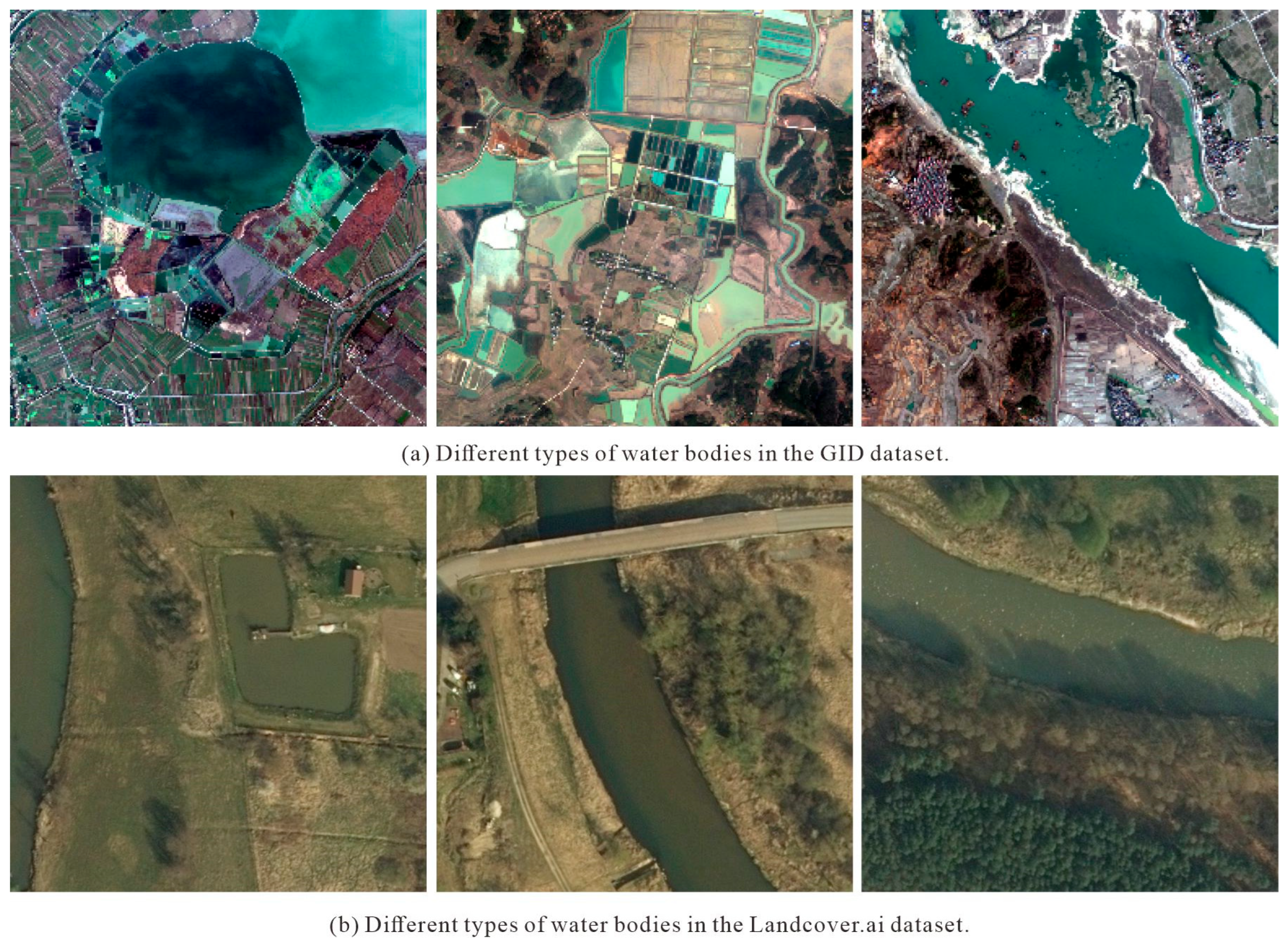
Figure 1. Schematic diagram of dataset samples.
Water 17 02760 g001
Figure 2. The structure chart of A2DSC-Net. (a) The basic architecture of A2DSC-Net. (b) The Res2Net Layer. (c) The MBDC module. (d) The A2-DSC module.
Water 17 02760 g002
Figure 3. Illustrations of 3 × 3 dilated convolution kernels with different dilatation rates of 1, 3, and 5. The yellow areas depict the effective receptive field, while the blue blocks represent the central positions of the convolutional kernels.
Water 17 02760 g003
Figure 4. Schematic diagram of DSConv receptive field.
Water 17 02760 g004
Figure 5. Visualization of ablation studies on the GID dataset. (ae) represent five distinct types of water bodies with different environmental conditions and distribution patterns. The red circled areas indicate the locations where different models are prone to misclassification and omission during water body extraction.
Water 17 02760 g005
Figure 6. Visualization of ablation studies on the LandCover.ai dataset. (ae) represent five distinct types of water bodies with different environmental conditions and distribution patterns. The red circled areas indicate the locations where different models are prone to misclassification and omission during water body extraction.
Water 17 02760 g006
Figure 7. Visualization of comparative studies on the GID dataset. (ae) represent five distinct types of water bodies with different environmental conditions and distribution patterns. The red circled areas indicate the locations where different models are prone to misclassification and omission during water body extraction.
Water 17 02760 g007
Figure 8. Visualization of comparative studies on the LandCover.ai dataset. (ae) represent five distinct types of water bodies with different environmental conditions and distribution patterns. The red circled areas indicate the locations where different models are prone to misclassification and omission during water body extraction.
Water 17 02760 g008
Table 1. Ablation experiment on the GID dataset.
MethodPrecision (%)Recall (%)IoU (%)F1-Score (%)
baseline95.9594.3390.7295.13
Baseline-MBDC95.594.890.7595.15
Baseline-A2DSC95.2394.9390.6395.08
A2DSC-Net95.6995.2991.3795.49
Table 2. Ablation experiment on the LandCover.ai dataset.
MethodPrecision (%)Recall (%)IoU (%)F1-Score (%)
baseline97.4794.5692.395.99
Baseline-MBDC97.295.5993.0296.38
Baseline-A2DSC96.9196.8593.9596.88
A2DSC-Net96.9897.0894.2397.03
Table 3. Comparative experiment on the GID dataset.
MethodPrecision (%)Recall (%)IoU (%)F1-Score (%)
DeepLabv3+92.5894.3387.793.45
U-Net95.494.8990.7495.15
PSPNet93.2492.0986.3392.66
DANet95.3691.687.6993.44
A2DSC-Net95.6995.2991.3795.49
Table 4. Comparative experiment on the LandCover.ai dataset.
MethodPrecision (%)Recall (%)IoU (%)F1-Score(%)
DeepLabv3+92.794.7788.1993.72
U-Net96.6194.5691.5295.57
PSPNet96.1895.1191.6595.64
DANet96.3595.391.9895.82
A2DSC-Net96.9897.0894.2397.03
Disclaimer/Publisher’s Note: The statements, opinions and data contained in all publications are solely those of the individual author(s) and contributor(s) and not of MDPI and/or the editor(s). MDPI and/or the editor(s) disclaim responsibility for any injury to people or property resulting from any ideas, methods, instructions or products referred to in the content.