Article

Developing Rainfall Spatial Distribution for Using Geostatistical Gap-Filled Terrestrial Gauge Records in the Mountainous Region of Oman

1
Egyptian Ministry of Water Resources and Irrigation, Port Said 42511, Egypt
2
Civil Engineering Department, Faculty of Engineering, Port Said University, Port Said 42523, Egypt
3
Division of Water Resources Engineering, Lund University, P.O. Box 118, 22100 Lund, Sweden
4
Centre for Advanced Middle Eastern Studies, Lund University, P.O. Box 201, 22100 Lund, Sweden
5
Irrigation and Hydraulics Department, Faculty of Engineering, Cairo University, Giza 12613, Egypt
*
Authors to whom correspondence should be addressed.
Water 2025, 17(18), 2695; https://doi.org/10.3390/w17182695
Submission received: 11 August 2025 / Revised: 3 September 2025 / Accepted: 9 September 2025 / Published: 12 September 2025
(This article belongs to the Section Hydrology)

Abstract

Arid mountainous regions are vulnerable to extreme hydrological events such as floods and droughts. Providing accurate and continuous rainfall records with no gaps is crucial for effective flood mitigation and water resource management in these and downstream areas. Satellite data and geospatial interpolation can be employed for this purpose and to provide continuous data series. However, it is essential to thoroughly assess these methods to avoid an increase in errors and uncertainties in the design of flood protection and water resource management systems. The current study focuses on the mountainous region in northern Oman, which covers approximately 50,000 square kilometers, accounting for 16% of Oman’s total area. The study utilizes data from 279 rain gauges spanning from 1975 to 2009, with varying annual data gaps. Due to the limited accuracy of satellite data in arid and mountainous regions, 51 geospatial interpolations were used to fill data gaps to yield maximum annual and total yearly precipitation data records. The root mean square error (RMSE) and correlation coefficient (R) were used to assess the most suitable geospatial interpolation technique. The selected geospatial interpolation technique was utilized to generate the spatial distribution of annual maxima and total yearly precipitation over the study area for the period from 1975 to 2009. Furthermore, gamma, normal, and extreme value families of probability density functions (PDFs) were evaluated to fit the rain gauge gap-filled datasets. Finally, maximum annual precipitation values for return periods of 2, 5, 10, 25, 50, and 100 years were generated for each rain gauge. The results show that the geostatistical interpolation techniques outperformed the deterministic interpolation techniques in generating the spatial distribution of maximum and total yearly records over the study area.

1. Introduction

Spatial rainfall distribution plays a significant role in hydrological studies. It has important impacts on, e.g., floods occurrence, crop production, urban drainage systems, and hydraulic structures design. It also influences decision-making and risk assessment in environmental management. Arid regions are especially vulnerable to extreme hydrological events such as floods and droughts [1]. Providing accurate and gap-free rainfall records is vital for effective flood mitigation and water resource management in these and the downstream areas. However, these areas often suffer from insufficient precipitation records. To overcome this challenge, more advanced techniques such as satellite data and geostatistical interpolation need to be utilized. These methods, however, should be assessed and validated to optimize the design processes in water resource management.
Water scarcity is a global challenge for human development and the achievement of economic goals. The world is suffering from increasing demand of water resources due to the increase in urbanization, industrial activities, the world’s human population, and the overexploitation of aquifers [2,3]. In total, 700 million people suffer from the shortage of drinking water, and more than 40% of the world’s population suffers from water scarcity [4]. The increasing stress of water resources in arid regions due to the increasing population and climate change causes increasing water scarcity [2]. Moreover, the occurrence of floods poses a threat to lives and economics. On 10 September 2023, storm Daniel caused landfall in Libya. The massive flooding killed more than 4300 people, while more than 8500 people are still missing. On 7 March 2024, deadly floods struck West Sumatra in Indonesia, leading to the damage of homes and forcing people to migrate. The maximum yearly precipitation forms the backbone for the design of flood mitigation measures, while the total yearly precipitation is fundamental for sustainable water resource management. Filling the gaps in rainfall data can contribute to managing the water resources and meeting the increasing needs of fresh water resources.
Rainfall distribution is affected by mountainous terrain. The complex topography of mountainous regions makes the spatial rainfall distribution different from plain regions [5]. There are different spatial interpolation methods used to model rainfall that depend on the data of sparse stations to predict rainfall distribution but differ in their mathematical concepts. Spatial interpolation predicts values at locations with no observations [6]. Interpolation methods can be divided into two main groups: deterministic and geostatistical approaches. Deterministic interpolation techniques, like inverse distance weighting and Thiessen polygons, specify values to locations according to the neighboring observed values and to mathematical formulas that set the degree of smoothness of the generated surface. Geostatistical methods like kriging depend on statistical models that contain autocorrelation (statistical relationship among the measured points). Hence, geostatistical approaches not only generate a prediction surface but also provide some measure of the accuracy of the estimations. Deterministic methods do not use probability theory or an indication of the extent of possible errors, while geostatistical methods provide probabilistic estimates or use the concept of randomness [7,8]. Kriging is the most used geostatistical method for spatial interpolation, in which the neighboring observed values are weighted to produce an estimated value for an unmeasured point. Weights depend on the distance between the observed locations, the estimation points, and the spatial arrangement among the observed points. The weights are calculated such that points nearby to target locations are given more weight than those farther away. Kriging methods do not only consider the distance between the measured values but also capture the spatial structure in the data; they depend on a spatial model between observations defined by a variogram. Kriging methods are divided into two categories: univariate and multivariate methods. The methods that can use secondary information are called “multivariate”, while those that ignore secondary information are known as “univariate” methods [9]. Table 1 shows a summary of different geostatistical and deterministic interpolation techniques, while Table 2 presents univariate and multivariate kriging methods.
A variogram is a visual representation of the covariance between each two points in the sampled data, also called a semivariogram. The semivariance (i.e., gamma value) is the value of the half mean-squared difference between observations. The semivariance is plotted against the distance (i.e., lag) between each two points in the sampled data [10]. There are different variogram models, while the most commonly used are exponential, spherical, linear, Gaussian, and circular [11].
Spatial interpolation of annual rainfall was performed in South Africa using different interpolation techniques (universal kriging, ordinary kriging, co-kriging, and IDW); however, the cross-validation was applied to determine the best interpolation approach [12]. The best performance was produced by ordinary kriging. The results showed that the kriging methods outperformed IDW. For the variogram models, the circular model was the best regardless of the technique used. Kyriakidis et al. [13] conducted a study to map rainfall distribution from rain gauge data using different interpolation techniques in the coastal region of northern California that has the characteristics of extreme seasonal variability in rainfall and complex terrain topography. The results showed that using secondary information such as terrain and atmospheric characteristics in predicting the rainfall distribution could improve estimates and result in more accurate representations of rainfall distribution. Moreover, the magnitude of estimation improvement depends on the spatial variability of the rainfall field, the density of rain gauge stations, and the degree of correlation between rainfall and predictors.
Sadeghi et al. [14] performed a study to predict rainfall distribution in Iran. The study used the average data of rainfall from 35 stations and rainfall observations for the period from 1982 to 2012 using different interpolation methods (i.e., kriging, co-kriging, local polynomial interpolation, global polynomial interpolation, RBF, and IDW). These techniques were evaluated using cross-validation. The results showed that the simple co-kriging (exponential) method was the most suitable method to predict rainfall distribution over the study area, while IDW with power 5 had the poorest performance. The study found that correlation existed between elevation variations and the precision of co-kriging method. Haberlandt [15] applied multivariate methods (i.e., indicator kriging with an external drift (IKED) and kriging with an external drift (KED)) to predict the spatial distribution of hourly rainfall from rain gauges with the use of secondary information from elevation, rainfall from a daily network, and radar, in a region of 25,000 km2 in southeast Germany. The cross-validation method was utilized to compare the performances of IKED and KED incorporating secondary information with univariate techniques (Thiessen polygon, IDW, ordinary indicator kriging (IK), and ordinary kriging (OK)). The results showed that the multivariate techniques IKED and KED obviously outperformed the univariate techniques due to the use of secondary information from elevation, daily rainfall from the network, and radar. In addition, the best result was produced when all secondary information were utilized together with KED.
Rata et al. [16] compared three interpolation approaches to mapping the annual rainfall distribution of Cheliff watershed, Algeria. The mean annual rainfall data with elevation from 58 stations for the period from 1972 to 2012 were used during the study. Moreover, OK, KED, and regression kriging (RK) were considered for the study. The interpolation approaches used were compared utilizing the cross-validation method. It was found that KED was the best interpolation technique to represent mean annual rainfall distribution for the study area. Goovaerts [17] used three multivariate interpolation methods (co-located co-kriging, kriging with an external drift, and simple kriging with varying local means) to incorporate elevation into the spatial interpolation of rainfall in a region of 5000 km2 in Portugal. The data of monthly and annual rainfall from 36 climatic stations were used, and cross-validation was also utilized to compare the multivariate methods with three univariate ones (ordinary kriging, inverse square distance, and Thiessen polygon). The results showed that the three multivariate interpolation methods outperformed the univariate ones, as higher prediction errors were produced by the univariate techniques that ignore rainfall measurements at neighboring stations and elevation.
Frequency analysis is utilized to estimate the periodic occurrence of quantities of rainfall that are predicted in the future. Data from rainfall frequency analysis are vital for many sectors of water resource engineering such as dam and sewage system design and flood mitigation [18,19]. Rainfall frequency analysis is often performed with the use of maximum yearly rainfall series [20]. The quantity of rainfall over a certain location in each period is characterized by a high variation in time. This variation is dependent on, e.g., the length of the given period, climate type, and topographic conditions. Arid areas usually display higher variation. Normally, management and design of flood mitigation systems, hydraulic structures, and irrigation water supply are dependent on rainfall amounts that are predicted for a certain return period. This rainfall is determined using frequency analysis of long time series [21]. The return period in the frequency analysis of precipitation is the average time interval between the occurrence of rainfall with a specific quantity or intensity [22]. Rainfall records in frequency analysis are considered random variables that are based on identical distribution and independent variables [21,22]. The frequency analysis is performed using different probability distributions such as two-parameter distributions (gamma and Gumbel) and three-parameter distributions (generalized Pareto (GPA), Pearson type III (PE-III), generalized normal (GNO), generalized extreme value (GEV), and log-Pearson type III (LP-III)) [23].
For the determination of the goodness of fit for probability distributions, the chi-squared test can be utilized [24,25]. The Akaike Information Criterion (AIC) and Bayesian Information Criterion (BIC) are also commonly utilized techniques for model selection [26,27]. Assessment of the performance of probability distributions for the frequency analysis of rainfall was carried out utilizing rainfall data for the period from 1973 to 2012 for Dois Vizinhos, Brazil [28]. The study showed that Weibull and gamma distribution were the most suitable. Waghaye et al. [29] compared probability distributions for monthly rainfall data from 1972 to 2001 at Adilabad district of Telangana, India. The chi-squared test was conducted, and the gamma, GEV, and Gumbel distributions were the best. Yuan et al. [30] identified five probability distributions (i.e., gamma, Gumbel, normal, log-Pearson type III, and log-normal) to predict the frequency analysis of annual maximum hourly rainfall for the period from 1981 to 2000 for 15 locations in Japan. The chi-squared test was considered for evaluating the goodness of fit. It was found that log-Pearson type III was the most suitable for the data.
Based on the above, it is obvious that geospatial interpolation is important to overcome insufficient rainfall gauge data, especially in arid mountainous regions. Therefore, the objectives of the current study were (1) using different geospatial interpolation models to fill the precipitation data gaps in the mountainous region in arid northern Oman based on data from 279 rain gauges spanning from 1975 to 2009, (2) comparing the performance of the investigated geospatial interpolation methods, (3) generating spatial distributions for annual maximum and total annual rainfall over the study area using different geospatial interpolation techniques, and (4) performing frequency analysis on the annual maximum rainfall considering different probability distributions to produce predictions for the annual maximum rainfall with different return periods over the study area.

2. Materials and Methods

2.1. Study Area

Oman is located in the southeastern quarter of the Arabian Peninsula with a 309,500 km2 land area. Several catchments are characterized by a mountainous terrain. The selection of the current study catchments was based on the availability of flood volume field measurements and corresponding rain gauge records. The study area is over 80,000 km2 and contains 279 rain gauges. The weather of Oman is hot and dry in summer, moderately cool in winter, hot and humid for coastal areas, and moderate and rainy for highlands. The temperature exceeds 40 °C for the period from April to August and decreases gradually from September to February, the temperature reaches 5 to 10 °C for mountainous regions in winter and decreases below these at extreme heights. Figure 1 shows a topographic map of the study area. Figure 2 shows the distribution of rain gauge stations over the study area.

2.2. Rain Gauge Records

There are potentially 279 rain gauges in the study area that have been in operation from 1975 to 2009, but the actual available data in each year can be sparse. Table 3 shows the available data from rain gauge stations for each year.

2.3. Geospatial Interpolation Methods

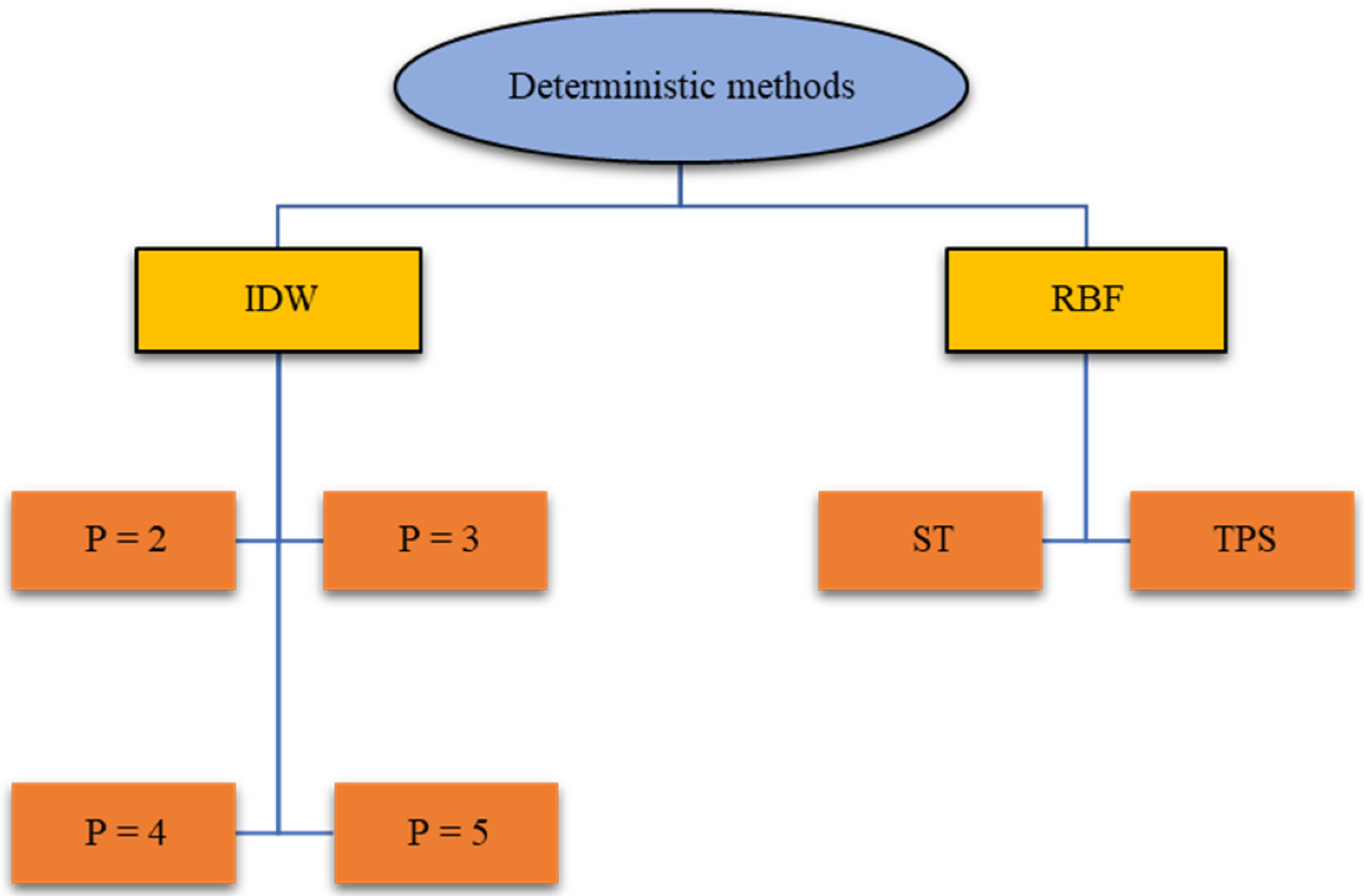
Geospatial interpolation was utilized to generate the spatial distribution of precipitation. These methods include two categories: geostatistical and deterministic techniques. The selected geospatial interpolation methods (Figure 3 and Figure 4) were utilized to fill gaps in data and produce the spatial distribution for total and annual daily maximum rainfall over the study area. Cross-validation was utilized to evaluate the interpolation methods, observations were excluded from the study area, and then the values at these points were estimated using the remaining data. Root mean square error (RMSE) and correlation coefficient (R) were calculated for the assessment of the performance of the interpolation techniques. The lower the value of RMSE, the higher the accuracy of the interpolation method. The higher the value of R, the higher the accuracy of the interpolation method [7,31]. We used two deterministic methods (inverse distance weighting (IDW) and radial basis function (RBF)) and seven geostatistical methods (empirical Bayesian kriging (EBK), ordinary kriging (OK), ordinary co-kriging (OCK), simple kriging (SK), simple co-kriging (SCK), universal kriging (UK), and universal co-kriging (UCK)). For IDW, the power values 2, 3, 4, and 5 were used. For the RBF, the basic functions spline with tension (ST) and thin-plate spline (TPS) were used. For EBK, the variograms linear (L), power (P), and thin-plate spline (TPS) were used. For kriging, the variogram models circular, exponential, Gaussian, J Bessel, K Bessel, spherical, and stable were used. For co-kriging, elevation was incorporated as a secondary variable to improve estimates. ArcGIS 10.8 software was utilized to generate the spatial rainfall distribution maps for the study area. After interpolation, missing rainfall value gaps were filled in. Spatial rainfall distribution maps of annual and annual maximum daily were generated for each year.

2.3.1. Inverse Distance Weighting (IDW)

IDW is one of the most used deterministic interpolation methods. The main assumption in this method is that the weight values are inversely proportional to the powers of the distance between the interpolation points and the measurement point, and the measured values at a closer distance have a greater weight than those further away [32,33]. IDW calculates cell values based on a linearly weighted combination of a group of sampled points as [32]:
Z ( x 0 ) = i = 1 n x i d i j r i = 1 n 1 d i j r
where Z(x0) is the predicted value, x is the set of spatial coordinates (x1, x2), and r is the weight related to the distance dij between the prediction of the n data points.

2.3.2. Radial Basis Function (RBF)

The RBF is a deterministic method in which the interpolated surface requires passing through every measured point. Examples of basic functions are spline with tension (ST), thin-plate spline (TPS), inverse multiquadric function (IMQ), multiquadric function (MQ), and completely regularized spline (CRS) [32,34]. The main difference between IDW and the RBF is that IDW is based on the extent of similarity, while the RBF is based on the degree of smoothness [35]. IDW cannot estimate values above maximum measured values or below minimum measured values, while the RBF estimates values higher than the highest measured values and lower than the minimum measured values [36,37].

2.3.3. Ordinary Kriging (OK)

OK is the most used kriging method. It estimates the value of a point where a variogram is known with the use of the data in the neighborhood of the predicted point. A block value can be estimated using OK in lieu of a point value [38]. It uses an average of a group of neighboring points in order to produce a particular interpolation point. OK is based on the assumption that there is spatial autocorrelation between the points in the domain. Based on this relationship, the measured values at the points separated by short distances are more similar than those measured at the points separated by larger distances [38,39]. Using OK supposes estimating a value at x0 using the values of the data points. The neighboring sampled points xα are combined linearly with weights wα as:
z O K * ( x 0 )   =   α = 1 n w α z ( x α )
where z O K * is the predicted value at the target point x0, z is the measured value at the data point xα, wα is the weight attached to the data point, and n is the number of the data points utilized for the estimation. The weights assigned to the data points should sum to unity (Equation (3)); hence, if all values are equal to a constant, this will result in the predicted value being constant [38,40]:
α = 1 n w α   =   1

2.3.4. Simple Kriging (SK)

SK utilizes the average of all the sampled data. This produces less accuracy compared to OK; however, it results in a smoother result. It considers that the data have a known constant mean value throughout the study area, and the weights assigned to values do not sum to unity [32,41,42]. Let Z(xα) be a random variable at each of the data locations Xα and let Z(x0) be a random variable at the target point X0. These random variables are assumed as a subset of an infinite collection of random variables called a random function Z(x) and the random function is assumed as second-order stationary. The expectation and the covariance are both translation-invariant over the domain. Assuming a vector h linking any two points x and x + h in the domain:
E[z(x + h)] = E[z(x)]
cov[z(x + h), z(x)] = c(h)
The expected value E[z(x)] = m is the same at any point x of the domain. The covariance between any two points is based on the vector h that links them. The aim is to form a weighted average to produce an estimation of the value at the target location X0 based on information at data locations Xα; α = 1:n. This estimation procedure requires determining the covariances between the random variables at the points of the domain. This process is like multiple regression transposed into a spatial context where Z(xα) performs like a regressor in regression with Z(x0). The spatial regression is defined as SK, which has a mean m that is constant through the domain. This mean m is calculated as the average of the data [38].

2.3.5. Empirical Bayesian Kriging (EBK)

EBK is different from other kriging methods as it accounts for the error in estimating the variogram through repeated simulations, it uses many variogram models instead of a single variogram. This process includes the following steps [43]:
  • EBK estimates a variogram model using information on the data.
  • EBK simulates a new value at input data locations based on the estimated variogram.
  • The simulated data are used to estimate a new variogram model. Bayes’ rule is used to calculate the weight of this variogram.
  • With every repetition of steps (2 and 3), a new group of values at the input data locations is simulated using the estimated variogram in step 1.
  • A new variogram model and its weights are estimated using the simulated data. These weights are utilized to generate predictions and prediction standard errors at the unsampled points.

2.3.6. Universal Kriging (UK)

UK is mostly utilized with data that have a considerable spatial trend, like a sloping surface. It relaxes the assumption of stationarity as it allows the mean of values to differ in a deterministic way in different locations (through some kind of spatial trend), while only the variance remains constant through the whole field [10,38,44]. UK is an extension of OK. The mean in OK is assumed to be constant through the search window, but in some cases the mean may not be constant due to the existence of a local trend, which results in the mean being a function of the local trend (coordinates). UK incorporates the local trend through the neighborhood search window as a function of the coordinates. The estimated value at the target point X0 is represented by UK as a deterministic function of spatial coordinates as [9,45,46]:
z*(x0) = μ(x0) + ε(x0)
where z*(x0) is the predicted value at the target point x0, μ(x0) is a deterministic function that varies smoothly, and ε(x0) is stochastic residuals.

2.3.7. Co-Kriging

Co-kriging is a geostatistical method that is used when a secondary variable is cross-correlated with the target variable, then both variables are used for estimation using co-kriging. The additional observed variables (known as covariates, which are often correlated with the target variable) are utilized to improve the precision of the interpolation of the target variable. Information on secondary variables is utilized to decrease the estimation variance of the target variable. Co-kriging outperforms kriging considering the accuracy of the estimations and the costs in the case that the random fields under study are cross-correlated [47,48]. The expression of co-kriging can be represented as [9,49]:
z 1 * ( x 0 )     μ 1   =   i 1 = 1 n 1 w i 1 [ z 1 ( x i 1 )     μ 1 ( x i 1 ) ]   +   j = 2 n v i j = 1 n j w i j [ z j ( x i j )     μ j ( x i j )]
where z 1 * ( x 0 ) is the predicted value at the target point x0, μ1 is a known stationary mean of the target variable, z1( x i 1 ) is the data of the target variable at point i1, μ1( x i 1 ) is the mean of sampled points through the search window, n1 is the number of samples through the search window for point x0 used to make the prediction, w i 1 is the weights used to reduce the estimation variance of the target variable, nv is the number of secondary variables, nj is the number of jth secondary variable through the search window, w i j is the weights selected to be attached to the i j t h point of jth secondary variable, zj( x i j ) is the data at the i j t h point of the jth secondary variable, and μj( x i j ) is the mean of the sampled points of the jth secondary variable through the search window.
Simple Co-Kriging (SCK)
SCK basically depends on determining the means of the variables. Therefore, the value of a variable at a certain point is predicted with no need for data on the variable in the neighborhood [38]. By substituting μ1( x i 1 ) with μ1, and substituting μj( x i j ) with the stationary mean μj of secondary variables in Equation (7), the estimator of simple co-kriging can be obtained [9,49], which can be represented as:
z 1 * ( x 0 )   =   i 1 = 1 n 1 w i 1 [ z 1 ( x i 1 )     μ 1 ]   +   μ 1   +   j = 2 n v i j = 1 n j w i j [ z j ( x i j )     μ j ] =   i 1 = 1 n 1 w i 1 [ z 1 ( x i 1 ) ]   +   j = 2 n v i j = 1 n j w i j zj ( x i j )   +   ( 1     i 1 = 1 n 1 w i 1 )   μ 1     j = 2 n v i j = 1 n j w i j μ j
The advantage of SCK is that there are no constraints on weights, which reduces the variance of estimation, and the estimates are unbiased [50].
Ordinary Co-Kriging (OCK)
OCK is based on the following equations:
z 1 * ( x 0 )   =   μ 1   +   ε 1 ( x 0 )
z 2 * ( x 0 )   =   μ 2   +   ε 2 ( x 0 )
where μ1 and μ2 are unknown constants, and ε1(x0) and ε2(x0) are two types of random errors. So, there is autocorrelation for each one and cross-correlation between them. OCK predicts z 1 * ( x 0 ) with the use of information on the covariate z 2 * ( x 0 ) in order to produce better prediction. The information on the target variable z1, cross-correlations between z1 and other variable types, and autocorrelation for z1 are utilized by OCK to produce more accurate estimations [38,51].
Universal Co-Kriging (UCK)
UCK is utilized to make predictions when dealing with multivariate random functions. It is routinely used in environmental studies when there is a spatially variable mean or a trend in the secondary or primary variables. It can make predictions in a configuration that constitutes a single location, multiple points, or a gradient [52,53].

2.4. Frequency Analysis

By using the generated gap-free data obtained from the selected geospatial interpolation method, frequency analysis was performed using commonly used probability distributions, which can be divided into two groups: Three-parameter distributions are generalized extreme value (GEV), log-normal three-parameter (LN3), and Pearson type III (P-III)). Two-parameter distributions are extreme value type 1 (EV1), log-normal (LN2), exponential (EXPN), gamma, and Weibull (WEI2) [54,55]. Each distribution is identified by a probability density function. Table 4 shows the functions of the probability distributions used. The maximum likelihood method (MLK) is utilized to choose the suitable parameters to optimize the likelihood of observations. Then, the chi-squared (x2) test is performed with a significance level of 5% for the assessment of the adequacy of the probability distribution.
The proposed probability distributions were utilized to make predictions for the maximum yearly rainfall in the future with different return periods. The Akaike Information Criterion (AIC) and Bayesian Information Criterion (BIC) were utilized to choose the suitable probability distribution for the data; the probability distribution that has the lowest AIC and BIC is the best to fit the data [27,57].
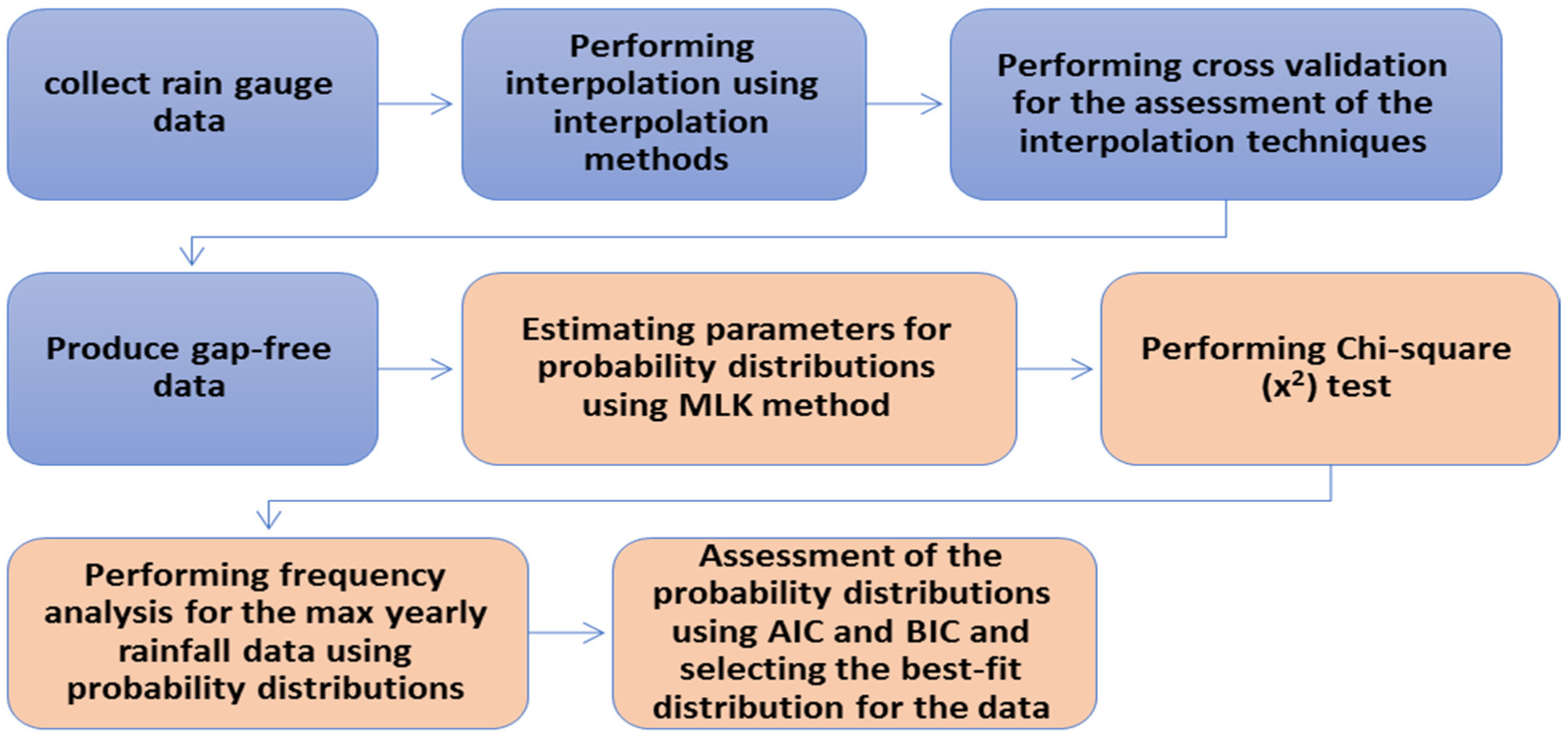
Figure 5 shows a schematic diagram for the applied procedure in the current study. First, the geospatial interpolation techniques were employed to fill the gaps in the data and generate the spatial distribution for annual maximum and total yearly precipitation over the study area. Secondly, the frequency analysis was performed using different probability distributions to make predictions for the maximum yearly rainfall in the future with different return periods.

3. Results and Discussion

The interpolation methods produced different spatial rainfall distribution patterns as shown in Figure 6; the colored legend goes from blue for low rainfall values to red for the highest rainfall values. Figure 6 shows a slight difference between the generated rainfall distribution pattern by each method, and the results showed that the OCK exponential method outperformed the other three methods (i.e., EBK L, OK stable, and RBF ST) in representing the spatial distribution of the maximum rainfall for year 1991 based on the cross-validation results, as it had a lower RMSE and a higher R.
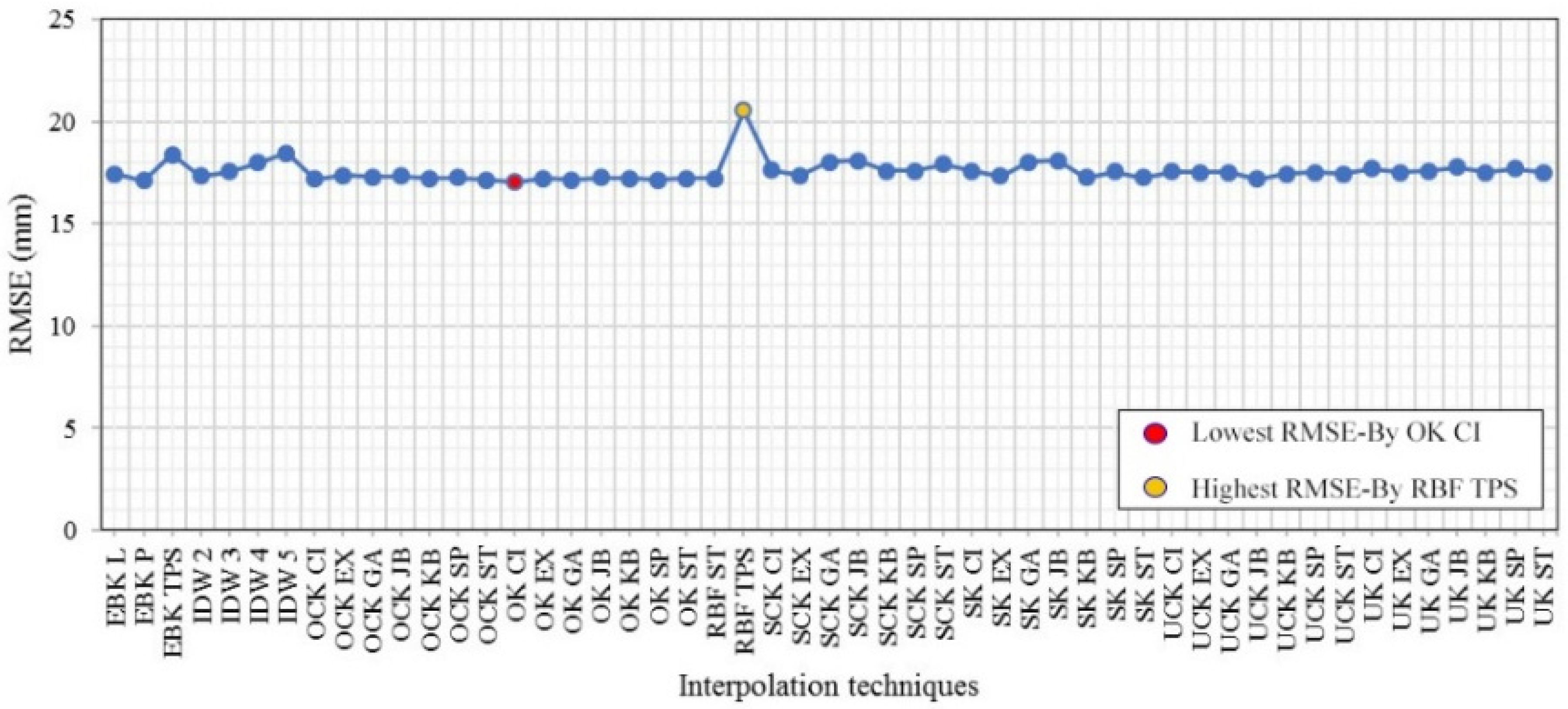
For maximum yearly rainfall interpolation, the results showed that the kriging methods outperformed the deterministic ones (IDW and RBF). IDW with power 2 outperformed the other power values. The spline with the tension basis function was more efficient than the thin-plate spline. In average, universal co-kriging using the J Bessel variogram model was superior to the other methods. The exponential model performed as well as the circular model, while the stable model had the lowest performance. IDW with power 5 and the RBF method with the thin-plate spline basis function had the poorest performance in predicting the rainfall distribution over the study area. The results of the cross-validation for the interpolation methods used for maximum rainfall for the year 1999 are shown in Table 5. Figure 7 and Figure 8 show the RMSE and R variability with interpolation methods for the maximum rainfall for the year 1999.
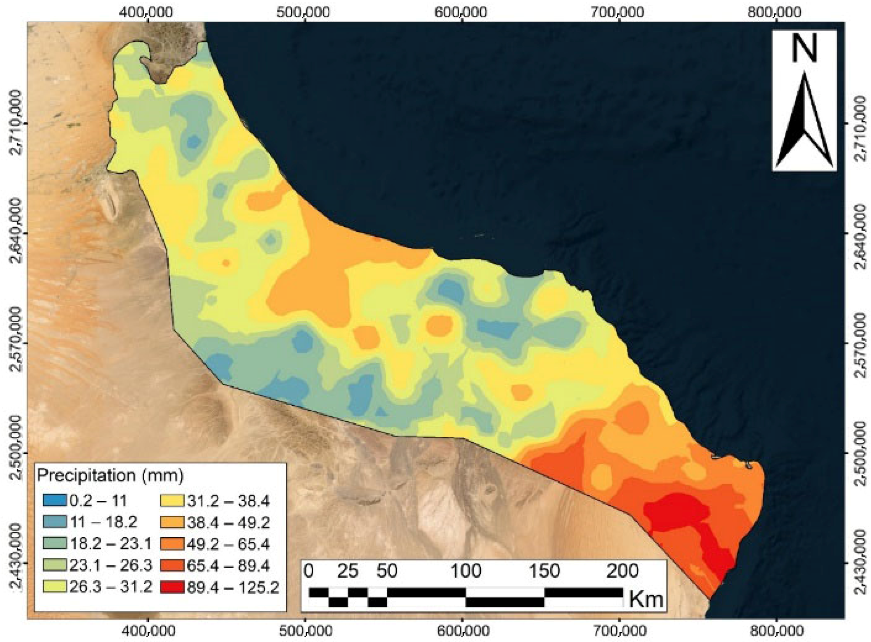
The results of maximum rainfall for 1999 showed that OK using circular variogram model was the best method at predicting the rainfall distribution as it had the lowest RMSE (17.02) and the highest R (0.63). Also, EBK P had the second best performance, with RMSE 17.11 and R 0.62. IDW with power 2 performed better than the other power values. For the RBF method, the spline with the tension basis function outperformed the thin-plate spline basis function. The RBF method with the thin-plate spline basis function had the poorest performance as it had the highest RMSE (20.53) and lowest R (0.52). Figure 7 and Figure 8 indicate that the RBF TPS method clearly produced less accuracy compared to other interpolation techniques, with the highest RMSE and lowest R. Figure 9 shows the spatial distribution of the maximum rainfall for the year 1999 produced by the OK circular method. The colored legend goes from blue for low rainfall values to red for the highest rainfall values. Figure 9 shows that the rainfall distribution is uneven, the western and northern areas show low rainfall values, while the high rainfall values are concentrated in the southern area. Table 6 shows the best interpolation method for annual daily maximum rainfall for each year for the period 1975–2009. In Table 6, it is clearly noted that geostatistical methods outperformed deterministic ones in predicting maximum yearly rainfall distribution over the study area.
For total annual rainfall interpolation, the kriging methods outperformed the deterministic ones (IDW and RBF). IDW with power 2 outperformed the other power values. The RBF method performed better than IDW. The spline with the tension basis function was more efficient than the thin-plate spline. On average, ordinary co-kriging and universal co-kriging using the K Bessel variogram model were superior to the other methods. The J Bessel and K Bessel variogram models performed well, while the Gaussian and exponential models had the lowest performance. IDW with power 5 and the RBF method with the thin-plate spline basis function had the poorest performance in predicting the rainfall distribution over the study area. The results of the cross-validation of the interpolation methods used for total rainfall for the year 2000 are shown in Table 7. Figure 10 and Figure 11 show the RMSE and R variability with interpolation method for the total rainfall for 2000.
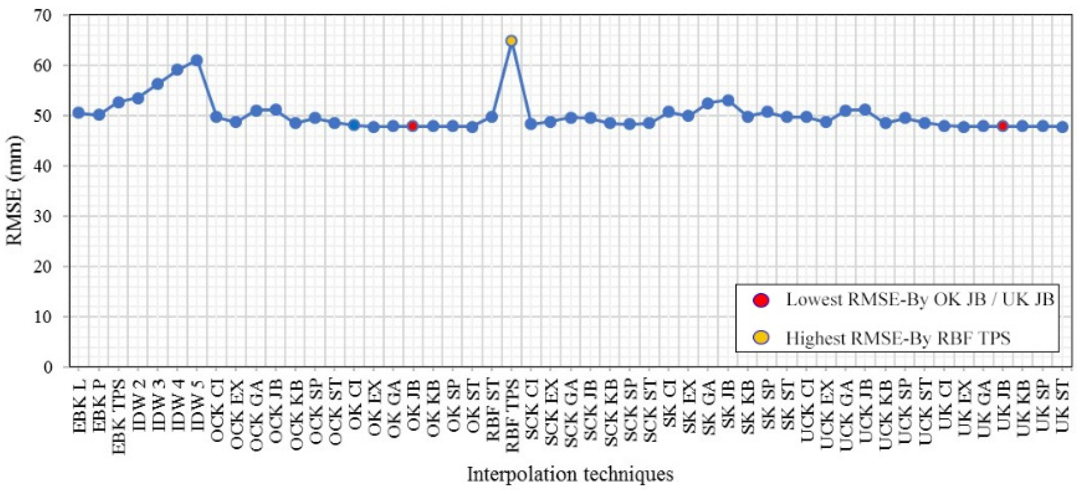
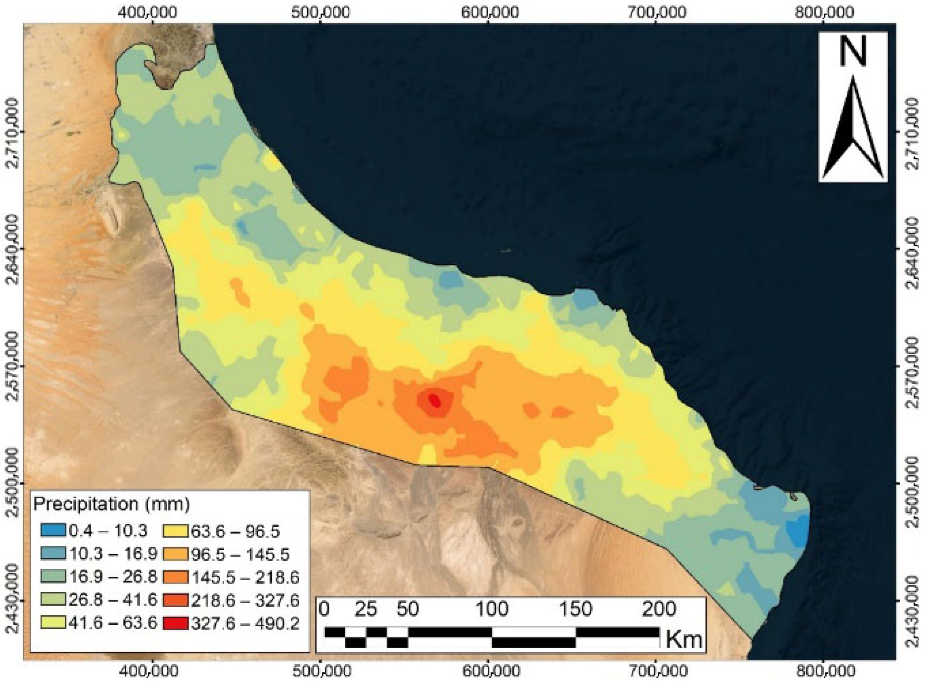
The results for the total annual rainfall in 2000 showed that OK using the J Bessel variogram model and UK with the J Bessel variogram had the best performance in predicting the rainfall distribution as they had the lowest RMSE (47.77 mm/year) and the highest R (0.81). Also, OK using the exponential variogram and UK with the exponential variogram performed similarly well. IDW with power 2 performed better than the other power values. For the RBF method, the spline with the tension basis function outperformed the thin-plate spline basis function. The RBF method with the thin-plate spline basis function had the poorest performance as it had the highest RMSE (64.82 mm/year) and the lowest R (0.69). It is noted from Figure 10 and Figure 11 that the RBF TPS method obviously had less accuracy with respect to other interpolation techniques, with the highest RMSE and the lowest R. Figure 12 shows the spatial distribution of the total rainfall for 2000 produced by the UK J Bessel method. The colored legend goes from blue for low rainfall values to red for the highest rainfall values. It appears from Figure 12 that the rainfall distribution is uneven; the northern and southern areas are of low rainfall values, while the high rainfall values are concentrated in the western area. Table 8 shows the best interpolation method for total yearly rainfall for each year for the period from 1975 to 2009. In general, the results obviously showed that geostatistical methods outperformed deterministic ones in predicting maximum yearly and total yearly rainfall over the study area. Figure 13 shows that for kriging methods, the J Bessel variogram model was superior to the other variogram models in predicting maximum yearly and total yearly rainfall over the study area regardless of the kriging method used, while the Gaussian model had the poorest performance.
A frequency analysis of the maximum yearly rainfall was performed for the original data and for the data after filling the gaps. For the original data analysis, 50 stations were excluded from the analysis as they had less than 10 records and they would not produce appropriate results. Table 9 shows the results of the frequency analysis of the original sampled rainfall data for return periods of 2, 5, 10, 25, 50, and 100 years. Table 10 shows the frequency analysis of the data after filling the gaps. It appears that the WEI2 distribution was the best to fit the data for both the original data analysis and gap-free data analysis as it had the lowest AIC and BIC.
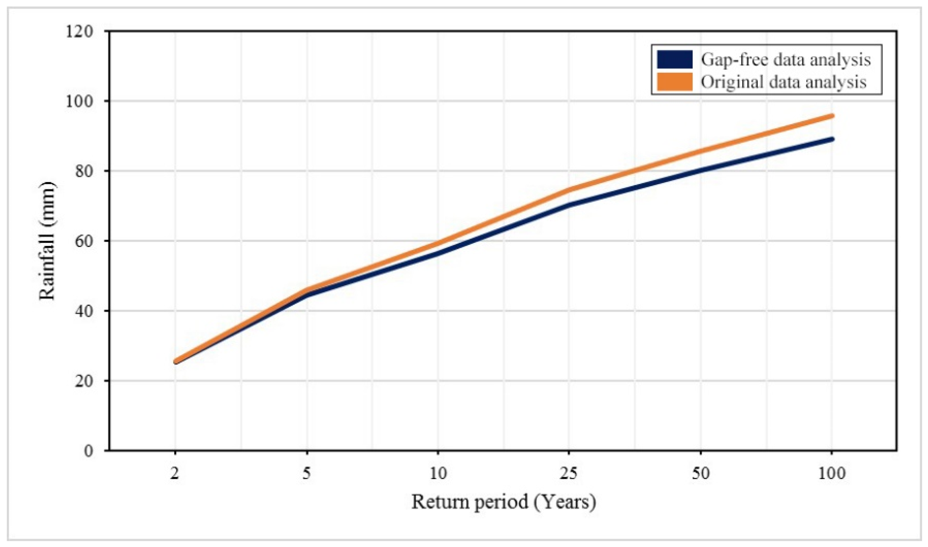
Figure 14 shows a comparison between the probability distributions in fitting the rainfall data. In general, the frequency analysis results showed that the WEI2 distribution was the best to fit the data, followed by the gamma distribution, while the LN3 distribution had the poorest performance. Table 11 shows the ratio between the average of the predicted rainfall values by the gap-free data analysis and the average of the predicted values by the original data analysis, it was noticed that for the return period of 2 years, the average of the predicted rainfall values using the original data analysis was lower than the average of the predicted rainfall values using the gap-free data analysis. Also, for the other return periods, the average of the predicted values using the original data analysis was higher than the average of the predicted values using the gap-free data analysis. Figure 15 represents the trend in the frequency analysis results for the original sampled data analysis and gap-free data analysis. It appears that for return periods greater than 2 years, the predicted rainfall value from the original data analysis was higher than that obtained by the gap-free data analysis.

4. Conclusions and Recommendations

In the current research, the performance of various interpolation methods in predicting the spatial distribution of rainfall over the mountainous region of Oman was evaluated. The results demonstrated that geostatistical interpolation techniques (i.e., SK, SCK, OK, OCK, UK, UCK, and EBK) outperformed deterministic interpolation techniques (i.e., IDW and the RBF) in generating the spatial distribution of maximum and total yearly records over the study area in Oman.
Universal co-kriging was the most effective method at predicting the maximum yearly rainfall distribution across the study area. On the other hand, both ordinary co-kriging and universal co-kriging showed comparable performance in interpolating the total yearly rainfall distribution in Oman. These findings highlight the reliability of co-kriging methods, particularly when incorporating additional variables such as elevation, for accurate spatial rainfall estimation in complex terrains. The J Bessel variogram outperformed the other six evaluated variograms (i.e., exponential, circular, Gaussian, stable, spherical, and K Bessel) in representing the spatial variance of the rainfall records.
The frequency analysis was conducted using data from the available rain gauges, and the two-parameter Weibull distribution outperformed the other seven tested statistical distributions (i.e., GEV, LN3, P-III, EV1, LN2, EXPN, and gamma) in predicting the design storm for different return periods (i.e., 2, 5, 10, 25, 50, and 100 years). The results indicated that for return periods greater than two years, the corresponding rainfall depth derived from the raw rain gauge data (before filling data gaps) was higher than that obtained from the gap-filled data. This suggests that flood protection design based on rainfall depths derived from raw data without gap filling is on the conservative side, ensuring a higher margin of safety.

Author Contributions

Conceptualization, Y.H., T.S., and A.M.H.; data curation, M.A.A.E.-B., and A.M.H.; formal analysis, M.A.A.E.-B., Y.H., T.S., and A.M.H.; funding acquisition, T.S., and R.B.; investigation, M.A.A.E.-B., Y.H., T.S., and A.M.H.; methodology, M.A.A.E.-B., and A.M.H.; project administration, Y.H., T.S., R.B., and A.M.H.; software, M.A.A.E.-B., and A.M.H.; supervision, Y.H., T.S., R.B., and A.M.H.; validation, M.A.A.E.-B., and A.M.H.; visualization, Y.H., T.S., R.B., and A.M.H.; writing—original draft, M.A.A.E.-B., T.S., and A.M.H.; writing—review and editing, Y.H., T.S., R.B., and A.M.H. All authors have read and agreed to the published version of the manuscript.

Funding

This research did not receive funding from specific agencies in the public, commercial, or not-for-profit divisions.

Data Availability Statement

The data presented in this study are available on request from the corresponding author.

Acknowledgments

This study was supported by the Middle East in the Contemporary World (MECW) project at the Centre for Advanced Middle Eastern Studies, Lund University.

Conflicts of Interest

The authors declare no conflicts of interest.

References

  1. El Kenawy, A.M. Hydroclimatic extremes in arid and semi-arid regions: Status, challenges, and future outlook. In Hydroclimatic Extremes in the Middle East and North Africa Assessment, Attribution and Socioeconomic Impacts; Elsevier: Amsterdam, The Netherlands, 2024; pp. 1–22. [Google Scholar] [CrossRef]
  2. Khan, M.Y.A.; ElKashouty, M.; Subyani, A.M.; Tian, F.; Gusti, W. GIS and RS intelligence in delineating the groundwater potential zones in Arid Regions: A case study of southern Aseer, southwestern Saudi Arabia. Appl. Water Sci. 2022, 12, 3. [Google Scholar] [CrossRef]
  3. Vaseashta, A. Introduction to Water Safety, Security and Sustainability BT. In Water Safety, Security and Sustainability: Threat Detection and Mitigation; Springer: Berlin/Heidelberg, Germany, 2021. [Google Scholar] [CrossRef]
  4. Shemer, H.; Wald, S.; Semiat, R. Challenges and Solutions for Global Water Scarcity. Membranes 2023, 13, 612. [Google Scholar] [CrossRef] [PubMed]
  5. Singh, P.; Ramasastri, K.S.; Kumar, N. Topographical influence on precipitation distribution in different ranges of western Himalayas. Nord. Hydrol. 1995, 26, 259–284. [Google Scholar] [CrossRef]
  6. Lanza, L.G.; Ramírez, J.A.; Todini, E. Stochastic rainfall interpolation and downscaling. Hydrol. Earth Syst. Sci. 2001, 5, 139–143. [Google Scholar] [CrossRef]
  7. Wijemannage, A.L.K.; Ranagalage, M.; Perera, E.N.C. Comparison of spatial interpolation methods for rainfall data over Sri Lanka. In Proceedings of the 37th Asian Conference on Remote Sensing, ACRS 2016, Colombo, Sri Lanka, 17–21 October 2016; Volume 3, pp. 1723–1732. [Google Scholar]
  8. Burrough, P.A.; McDonnell, R.A. Principles of Geographical Information Systems; Oxford University Press: Oxford, UK, 1998. [Google Scholar]
  9. Li, J.; Heap, A.D. A Review of Spatial Interpolation Methods for Environmental Scientists; Geoscience Australia: Symonston, Australia, 2008. Available online: http://www.ga.gov.au/image_cache/GA12526.pdf (accessed on 10 May 2024).
  10. Kriging Interpolation Explanation | Columbia Public Health | Columbia University Mailman School of Public Health. Available online: https://www.publichealth.columbia.edu/research/population-health-methods/kriging-interpolation (accessed on 18 May 2024).
  11. Aspexit, Variogram and Spatial Autocorrelation. 2019. Available online: https://www.aspexit.com/variogram-and-spatial-autocorrelation/ (accessed on 18 May 2024).
  12. Coulibaly, M.; Becker, S. Spatial interpolation of annual precipitation in South Africa—Comparison and evaluation of methods. Water Int. 2007, 32, 494–502. [Google Scholar] [CrossRef]
  13. Kyriakidis, P.C.; Kim, J.; Miller, N.L. Geostatistical mapping of precipitation from rain gauge data using atmospheric and terrain characteristics. J. Appl. Meteorol. 2001, 40, 1855–1877. [Google Scholar] [CrossRef]
  14. Sadeghi, S.H.; Nouri, H.; Faramarzi, M. Assessing the spatial distribution of rainfall and the effect of altitude in Iran (Hamadan Province). Air Soil Water Res. 2017, 10, 1–7. [Google Scholar] [CrossRef]
  15. Haberlandt, U. Geostatistical interpolation of hourly precipitation from rain gauges and radar for a large-scale extreme rainfall event. J. Hydrol. 2007, 332, 144–157. [Google Scholar] [CrossRef]
  16. Rata, M.; Douaoui, A.; Larid, M.; Douaik, A. Comparison of geostatistical interpolation methods to map annual rainfall in the Chéliff watershed. Algeria Theor. Appl. Climatol. 2020, 141, 1009–1024. [Google Scholar] [CrossRef]
  17. Goovaerts, P. Geostatistical approaches for incorporating elevation into the spatial interpolation of rainfall. J. Hydrol. 2000, 228, 113–129. [Google Scholar] [CrossRef]
  18. Chang, C.H.; Rahmad, R.; Wu, S.J.; Hsu, C.T. Spatial Frequency Analysis by Adopting Regional Analysis with Radar Rainfall in Taiwan. Water 2022, 14, 2710. [Google Scholar] [CrossRef]
  19. Gaál, L.; Kyselý, J.; Szolgay, J. Region-of-influence approach to a frequency analysis of heavy precipitation in Slovakia. Hydrol. Earth Syst. Sci. 2008, 12, 825–839. [Google Scholar] [CrossRef]
  20. Cheng, K.S.; Chen, B.Y.; Lin, T.W.; Nakamura, K.; Ruangrassamee, P.; Chikamori, H. Rainfall frequency analysis using event-maximum rainfalls—An event-based mixture distribution modeling approach. Weather. Clim. Extrem. 2024, 43, 100634. [Google Scholar] [CrossRef]
  21. Dirk, R. Frequency Analysis of Rainfall Data. 2013. Available online: https://indico.ictp.it/event/a12165/session/21/contribution/16/material/0/0.pdf (accessed on 14 May 2024).
  22. Alias, N.E.; Tarmizi, M.M.M.; Syazmi Chebby, M. Return Period Analysis of Major Flood Events Considering Homogeneous Regions. In Proceedings of the 4th Global Summit of Research Institutes for Disaster Risk Reduction, Kyoto, Japan, 13–15 March 2019; Springer: Singapore, 2023; pp. 281–291. [Google Scholar] [CrossRef]
  23. Zalina, M.D.; Desa, M.N.M.; Nguyen, V.T.V.; Kassim, A.H.M. Selecting a probability distribution for extreme rainfall series in Malaysia. Water Sci. Technol. 2002, 45, 63–68. [Google Scholar] [CrossRef]
  24. Baghel, H.; Mittal, H.K.; Singh, P.K.; Yadav, K.K.; Jain, S. Frequency Analysis of Rainfall Data Using Probability Distribution Models. Int. J. Curr. Microbiol. Appl. Sci. 2019, 8, 1390–1396. [Google Scholar] [CrossRef]
  25. Mohita Anand, S.; Jai Bhagwan, S. Use of Probability Distribution in Rainfall Analysis. N. Y. Sci. J. 2010, 3, 40–49. [Google Scholar]
  26. Laio, F.; Di Baldassarre, G.; Montanari, A. Model selection techniques for the frequency analysis of hydrological extremes. Water Resour. Res. 2009, 45, 1–11. [Google Scholar] [CrossRef]
  27. Chen, P.C.; Wang, Y.H.; You, G.J.Y.; Wei, C.C. Comparison of methods for non-stationary hydrologic frequency analysis: Case study using annual maximum daily precipitation in Taiwan. J. Hydrol. 2017, 545, 197–211. [Google Scholar] [CrossRef]
  28. Vieira, F.M.C.; Machado, J.M.C.; De Souza Vismara, E.; Possenti, J.C. Probability distributions of frequency analysis of rainfall at the southwest region of Paraná State, Brazil. Rev. Cienc. Agrovet. 2018, 17, 260–266. [Google Scholar] [CrossRef]
  29. Waghaye, A.M.; Siddenki, V.; Kumari, N.; Ingle, V.K. Design rainfall estimation using probabilistic approach for Adilabad district of Telangana. Eng. Technol. India 2015, 6, 1–11. [Google Scholar] [CrossRef]
  30. Yuan, J.; Emura, K.; Farnham, C.; Alam, M.A. Frequency analysis of annual maximum hourly precipitation and determination of best fit probability distribution for regions in Japan. Urban Clim. 2018, 24, 276–286. [Google Scholar] [CrossRef]
  31. Antal, A.; Guerreiro, P.M.P.; Cheval, S. Comparison of spatial interpolation methods for estimating the precipitation distribution in Portugal. Theor. Appl. Climatol. 2021, 145, 1193–1206. [Google Scholar] [CrossRef]
  32. Boumpoulis, V.; Michalopoulou, M.; Depountis, N. Comparison between different spatial interpolation methods for the development of sediment distribution maps in coastal areas. Earth Sci. Inform. 2023, 16, 2069–2087. [Google Scholar] [CrossRef]
  33. Types of Interpolation—Advantages and Disadvantages. Available online: https://gisresources.com/types-interpolation-methods_3/ (accessed on 18 May 2024).
  34. Biernacik, P.; Kazimierski, W.; Włodarczyk-Sielicka, M. Comparative Analysis of Selected Geostatistical Methods for Bottom Surface Modeling. Sensors 2023, 23, 3941. [Google Scholar] [CrossRef]
  35. ESRI. Deterministic Methods for Spatial Interpolation—ArcGIS Pro | Documentation. 2021. Available online: https://pro.arcgis.com/en/pro-app/latest/help/analysis/geostatistical-analyst/deterministic-methods-for-spatial-interpolation.htm (accessed on 18 May 2024).
  36. ESRI. How Radial Basis Functions Work—ArcGIS Pro | Documentation. Available online: https://pro.arcgis.com/en/pro-app/latest/help/analysis/geostatistical-analyst/how-radial-basis-functions-work.htm (accessed on 18 May 2024).
  37. Apaydin, H.; Kemal Sonmez, F.; Yildirim, Y.E. Spatial interpolation techniques for climate data in the GAP region in Turkey. Clim. Res. 2004, 28, 31–40. [Google Scholar] [CrossRef]
  38. Wackernagel, H. Multivariate Geostatistics; Springer: Berlin/Heidelberg, Germany, 2003. [Google Scholar] [CrossRef]
  39. Delbari, M.; Afrasiab, P.; Jahani, S. Spatial interpolation of monthly and annual rainfall in northeast of Iran. Meteorol. Atmos. Phys. 2013, 122, 103–113. [Google Scholar] [CrossRef]
  40. Zawadzki, J. Metody Geostatystyczne dla Kierunków Przyrodniczych i Technicznych [Geostatistical Methods for Natural and Technical Subjects]; Oficyna Wydawnicza Politechniki Warszwskiej: Warszawa, Poland, 2011. [Google Scholar]
  41. ESRI. GIS Dictionary. Available online: https://support.esri.com/en-us/gis-dictionary/search?q=simple+kriging (accessed on 18 May 2024).
  42. Viswanathan, R.; Jagan, J.; Samui, P.; Porchelvan, P. Spatial Variability of Rock Depth Using Simple Kriging, Ordinary Kriging, RVM and MPMR. Geotech. Geol. Eng. 2015, 33, 69–78. [Google Scholar] [CrossRef]
  43. Krivoruchko, K. Empirical Bayesian Kriging. ESRI Press Fall 2012, 2012, 6–10. [Google Scholar]
  44. ESRI. GIS Dictionary. Available online: https://support.esri.com/en-us/gis-dictionary/search?q=universal+kriging (accessed on 21 May 2024).
  45. Bostan, P. Basic kriging methods in geostatistics. Yuz. Yil Univ. J. Agric. Sci. 2017, 27, 10–20. [Google Scholar] [CrossRef]
  46. ESRI. Understanding Universal Kriging—ArcMap | Documentation. Available online: https://pro.arcgis.com/en/pro-app/latest/help/analysis/geostatistical-analyst/understanding-universal-kriging.htm (accessed on 18 May 2024).
  47. Giraldo, R.; Herrera, L.; Leiva, V. Cokriging prediction using as secondary variable a functional random field with application in environmental pollution. Mathematics 2020, 8, 1305. [Google Scholar] [CrossRef]
  48. Cokriging. Geospatial Data Science in R. Available online: https://zia207.github.io/geospatial-r-github.io/cokriging.html (accessed on 18 May 2024).
  49. Goovaerts, P. Geostatistics for Natural Resources Evaluation; Oxford University Press: New York, NY, USA, 1997. [Google Scholar]
  50. Minnitt, R.C.A.; Deutsch, C.V. Cokriging for optimal mineral resource estimates in mining operations. J. S. Afr. Inst. Min. Metall. 2014, 114, 189–203. [Google Scholar]
  51. ESRI. Understanding Cokriging—ArcMap | Documentation. Available online: https://desktop.arcgis.com/en/arcmap/latest/extensions/geostatistical-analyst/understanding-cokriging.htm (accessed on 18 May 2024).
  52. Stein, A.; van Eijnsbergen, A.C.; Barendregt, L.G. Cokriging nonstationary data. Math. Geol. 1991, 23, 703–719. [Google Scholar] [CrossRef]
  53. Dowd, P.A.; Pardo-Igúzquiza, E. The Many Forms of Co-kriging: A Diversity of Multivariate Spatial Estimators. Math. Geosci. 2024, 56, 387–413. [Google Scholar] [CrossRef]
  54. González-álvarez, Á.; Viloria-Marimón, O.M.; Coronado-Hernández, Ó.E.; Vélez-Pereira, A.M.; Tesfagiorgis, K.; Coronado-Hernández, J.R. Isohyetal maps of daily maximum rainfall for different return periods for the Colombian Caribbean Region. Water 2019, 11, 358. [Google Scholar] [CrossRef]
  55. Phien, H.N.; Arbhabhirama, A.; Sunchindah, A. Rainfall distribution in northeastern thailand. Hydrol. Sci. Bull. 1980, 25, 167–182. [Google Scholar] [CrossRef]
  56. Helmi, A.M.; Farouk, M.I.; Hassan, R.; Mumtaz, M.A.; Chaouachi, L.; Elgamal, M.H. Comparing Remote Sensing and Geostatistical Techniques in Filling Gaps in Rain Gauge Records and Generating Multi-Return Period Isohyetal Maps in Arid Regions—Case Study: Kingdom of Saudi Arabia. Water 2024, 16, 925. [Google Scholar] [CrossRef]
  57. Mohammed, E.A.; Naugler, C.; Far, B.H. Emerging Trends in Computational Biology, Bioinformatics, and Systems Biology; Morgan Kaufmann: Burlington, MA, USA, 2015; Available online: http://www.scopus.com/inward/record.url?eid=2-s2.0-84944594252&partnerID=tZOtx3y1 (accessed on 26 May 2024).
Figure 1. Topographic map of the experimental study area in Oman (elevation in m).
Water 17 02695 g001
Figure 2. Distribution of rain gauge in stations in the study area.
Water 17 02695 g002
Figure 3. The geostatistical interpolation methods used.
Water 17 02695 g003
Figure 4. The deterministic interpolation methods used.
Water 17 02695 g004
Figure 5. Schematic diagram for the applied procedure used to fill gaps in rainfall data.
Water 17 02695 g005
Figure 6. Examples of spatial distribution of annual daily maximum rainfall for 1991 over the study area in Oman using different interpolation methods: (A) EBK L, (B) OCK exponential, (C) OK stable, and (D) RBF ST.
Water 17 02695 g006
Figure 7. RMSE variability with interpolation methods for the annual daily maximum rainfall for 1999.
Water 17 02695 g007
Figure 8. Correlation coefficient (R) variability with interpolation methods for the annual daily maximum rainfall in 1999.
Water 17 02695 g008
Figure 9. Spatial distribution of the maximum daily rainfall for 1999 produced by the OK circular method.
Water 17 02695 g009
Figure 10. RMSE variability with interpolation method for the total annual rainfall in 2000.
Water 17 02695 g010
Figure 11. Correlation coefficient (R) variability with interpolation method for the total annual rainfall for year 2000.
Water 17 02695 g011
Figure 12. Spatial distribution of the total annual rainfall for year 2000 produced by UK J Bessel method.
Water 17 02695 g012
Figure 13. Comparison between the variogram models for kriging in predicting annual daily maximum and total annual rainfall over the study area for the period 1975–2009 regardless of the kriging method used.
Water 17 02695 g013
Figure 14. Comparison between the probability distributions in fitting the rainfall data.
Water 17 02695 g014
Figure 15. Trend in frequency for original and gap-free maximum annual rainfall.
Water 17 02695 g015
Table 1. Geostatistical and deterministic interpolation techniques.
GeostatisticalDeterministic
KrigingInverse distance weighting (IDW)
Co-krigingRadial basis function (RBF)
Empirical Bayesian krigingThiessen polygon
Local polynomial interpolation (LPI)
Global polynomial interpolation (GPI)
Table 2. Univariate and multivariate kriging methods.
UnivariateMultivariate
Simple kriging (SK)Universal kriging
Ordinary krigingSK with varying local means
Block krigingKriging with an external drift
Factorial krigingSimple co-kriging
Dual krigingOrdinary co-kriging
Table 3. Available Omani rainfall data from gauge stations.
YearNumber of Working StationsYearNumber of Working Stations
1975311993162
1976371994183
1977441995220
1978481996230
1979561997235
1980531998232
1981561999203
1982622000185
1983802001173
1984832002178
1985672003174
19861022004191
19871132005191
19881082006199
19891092007160
19901102008121
1991113200980
1992122
Table 4. Functions of probability distribution used [56].
NameProbability DistributionParameters
GEV f x = 1 α 1 k α x u 1 k 1 e x p 1 k α x u 1 k α , k , u
LN3 f ( x ) = 1 ( x m ) σ 2 π e x p l n x m μ 2 2 σ 2 μ , σ , m
P-III f ( x ) = 1 α β Γ β ( x γ ) β 1 e ( x γ α ) α , β , γ
EV1 f ( x ) = 1 α e x p x u α e x p x u α α , u
LN2 f ( x ) = 1 x σ 2 π e x p l n x μ 2 2 σ 2 μ , σ
EXPN f ( x ) = 1 α e x p x γ α α , γ
Gamma f ( x ) = 1 α β Γ β x β 1 e ( x α ) α , β
WEI2 f ( x ) = c α x α c 1 e x p x α c α , c
Table 5. Root mean square error (RMSE) and correlation coefficient (R) results for annual daily maximum rainfall for 1999.
Interpolation MethodRMSERInterpolation MethodRMSER
EBK L17.440.60SCK J Bessel18.110.56
EBK P17.110.62SCK K Bessel17.580.62
EBK TPS18.380.56SCK spherical17.600.59
IDW 217.310.61SCK stable17.890.58
IDW 317.550.60SK circular17.590.59
IDW 417.990.58SK exponential17.330.61
IDW 518.440.57SK Gaussian18.030.57
OCK circular17.180.62SK J Bessel18.080.56
OCK exponential17.350.61SK K Bessel17.260.62
OCK Gaussian17.290.61SK spherical17.560.60
OCK J Bessel17.320.61SK stable17.240.62
OCK K Bessel17.210.62UK circular17.690.59
OCK spherical17.270.61UK exponential17.520.60
OCK stable17.140.62UK Gaussian17.590.60
OK circular17.020.63UK J Bessel17.750.58
OK exponential17.200.62UK K Bessel17.530.60
OK Gaussian17.130.62UK spherical17.690.59
OK J Bessel17.240.62UK stable17.510.60
OK K Bessel17.200.62UCK circular17.560.60
OK spherical17.130.62UCK exponential17.510.60
OK stable17.220.62UCK Gaussian17.510.60
RBF ST17.230.62UCK J Bessel17.200.62
RBF TPS20.530.52UCK K Bessel17.430.61
SCK circular17.620.59UCK spherical17.520.60
SCK exponential17.370.61UCK stable17.440.60
SCK Gaussian18.000.57
Table 6. Best interpolation method for annual daily maximum rainfall for the period from 1975 to 2009.
YearBest Interpolation MethodYearBest Interpolation Method
1975IDW 21993OCK spherical
1976SK J Bessel1994UCK J Bessel
1977UCK J Bessel1995OCK exponential
1978UCK circular1996UCK stable
1979SK spherical1997OCK exponential
1980UCK J Bessel1998OCK K Bessel
1981SK Gaussian1999OK circular
1982OCK K Bessel2000UCK Gaussian
1983SCK circular2001RBF ST
1984SK circular2002EBK P
1985OK circular2003SK circular
1986SCK K Bessel2004SCK J Bessel
1987UCK J Bessel2005SCK Gaussian
1988OCK K Bessel2006UCK exponential
1989SK exponential2007UCK J Bessel
1990OCK J Bessel2008SK J Bessel
1991UCK J Bessel2009OK J Bessel
1992SCK stable
Table 7. Root mean square error (RMSE) and correlation coefficient (R) results for the total rainfall in 2000.
Interpolation MethodRMSERInterpolation MethodRMSER
EBK L50.540.78SCK J Bessel49.570.79
EBK P50.190.78SCK K Bessel48.470.80
EBK TPS52.710.76SCK spherical48.310.80
IDW 253.500.77SCK stable48.560.80
IDW 356.250.75SK circular50.750.78
IDW 459.080.74SK exponential49.920.79
IDW 561.060.72SK Gaussian52.500.76
OCK circular49.780.79SK J Bessel53.120.75
OCK exponential48.740.80SK K Bessel49.870.79
OCK Gaussian51.030.77SK spherical50.770.78
OCK J Bessel51.140.77SK stable49.770.79
OCK K Bessel48.510.80UK circular47.970.81
OCK spherical49.550.79UK exponential47.810.81
OCK stable48.570.79UK Gaussian47.860.81
OK circular47.970.81UK J Bessel47.770.81
OK exponential47.810.81UK K Bessel47.870.81
OK Gaussian47.860.81UK spherical47.920.81
OK J Bessel47.770.81UK stable47.820.81
OK K Bessel47.870.81UCK circular49.780.79
OK spherical47.920.81UCK exponential48.740.80
OK stable47.820.81UCK Gaussian51.030.77
RBF ST49.880.79UCK J Bessel51.140.77
RBF TPS64.820.69UCK K Bessel48.510.80
SCK circular48.290.80UCK spherical49.550.79
SCK exponential48.800.80UCK stable48.570.80
SCK Gaussian49.650.79
Table 8. Best interpolation method for total annual rainfall for the period from 1975 to 2009.
YearBest interpolation MethodYearBest interpolation Method
1975OCK circular/UCK circular1993OCK J Bessel/UCK J Bessel
1976OCK exponential/UCK exponential1994OCK stable/UCK stable
1977OCK K Bessel/UCK K Bessel1995OCK K Bessel/UCK K Bessel
1978OCK circular/UCK circular1996OCK stable/UCK stable
1979OCK J Bessel/UCK J Bessel1997OCK circular/UCK circular
1980SCK Gaussian/SCK stable1998OCK stable/UCK stable
1981RBF ST1999OCK Gaussian/UCK Gaussian
1982OCK K Bessel/UCK K Bessel2000OK J Bessel/UK J Bessel
1983OCK J Bessel2001RBF ST
1984SCK exponential2002OK J Bessel/UK J Bessel
1985UK J Bessel2003OCK spherical /UCK spherical
1986OCK stable/UCK stable2004SCK J Bessel
1987SK circular2005SCK J Bessel
1988OCK K Bessel/UCK K Bessel2006EBK P
1989OCK spherical /UCK spherical2007OCK circular/UCK circular
1990OCK K Bessel/UCK K Bessel2008RBF ST
1991OCK stable/UCK stable2009OCK J Bessel
1992OCK spherical/UCK spherical
Table 9. Frequency analysis of original sampled rainfall data (mm/year).
Station IDProbability
Distribution
Return Period (Years)AICBIC
25102550100
CM996898AFWEI225.5746.0359.1074.6785.5595.87306.06309.17
GEV25.5944.3257.6975.8090.15105.23310.97315.64
EV126.3944.3756.2771.3282.4893.55309.23312.34
LN325.1644.7758.8677.7892.60108.03310.30314.96
GAMMA24.6945.6460.1678.6992.47106.16306.77309.88
p-III25.3446.3461.0179.8293.85107.82308.19312.86
EXPN21.0547.8768.1694.97115.26135.55310.35313.46
LN221.9047.6971.62110.51146.24188.16312.89316.00
Table 10. Frequency analysis of gap-free sampled rainfall data (mm/year).
Station IDProbability
Distribution
Return Period (Years)AICBIC
25102550100
CM996898AFWEI225.3844.3956.3070.3280.0489.19302.90306.01
GEV26.0443.3754.7769.0679.6090.00308.02312.69
EV125.9743.3754.8969.4580.2590.97306.03309.14
LN325.4743.6155.9771.9484.0596.34307.55312.21
GAMMA24.3044.2858.0575.5788.56101.45304.21307.32
p-III24.9444.9558.8476.6089.82102.95305.85310.52
EXPN20.5546.6766.4392.56112.32132.08308.52311.63
LN221.6946.7069.73106.91140.90180.63311.20314.31
Table 11. Ratio between average of predicted rainfall from mean gap-free and original data.
Return period (years)25102550100
Ratio between gap-free and original data1.080.980.950.930.930.94
Disclaimer/Publisher’s Note: The statements, opinions and data contained in all publications are solely those of the individual author(s) and contributor(s) and not of MDPI and/or the editor(s). MDPI and/or the editor(s) disclaim responsibility for any injury to people or property resulting from any ideas, methods, instructions or products referred to in the content.