Article

Improving the Generalization Performance of Debris-Flow Susceptibility Modeling by a Stacking Ensemble Learning-Based Negative Sample Strategy

1
School of Civil Engineering, Chongqing University, Chongqing 400045, China
2
State Key Laboratory of Safety and Resilience of Civil Engineering in Mountain Area, Chongqing 400045, China
*
Author to whom correspondence should be addressed.
Water 2025, 17(16), 2460; https://doi.org/10.3390/w17162460
Submission received: 9 July 2025 / Revised: 10 August 2025 / Accepted: 16 August 2025 / Published: 19 August 2025
(This article belongs to the Special Issue Intelligent Analysis, Monitoring and Assessment of Debris Flow)

Abstract

To address the negative sample selection bias and limited interpretability of traditional debris-flow event susceptibility models, this study proposes a framework that enhances generalization by integrating negative sample screening via a stacking ensemble model with an interpretable random forest. Using Wenchuan County, Sichuan Province, as the study area, 19 influencing factors were selected, encompassing topographic, geological, environmental, and anthropogenic variables. First, a stacking ensemble—comprising logistic regression (LR), decision tree (DT), gradient boosting decision tree (GBDT), and random forest (RF)—was employed as a preliminary classifier to identify very low-susceptibility areas as reliable negative samples, achieving a balanced 1:1 ratio of positive to negative instances. Subsequently, a stacking–random forest model (Stacking-RF) was trained for susceptibility zonation, and SHAP (Shapley additive explanations) was applied to quantify each factor’s contribution. The results show that: (1) the stacking ensemble achieved a test-set AUC (area under the receiver operating characteristic curve) of 0.9044, confirming its effectiveness in screening dependable negative samples; (2) the random forest model attained a test-set AUC of 0.9931, with very high-susceptibility zones—covering 15.86% of the study area—encompassing 92.3% of historical debris-flow events; (3) SHAP analysis identified the distance to a road and point-of-interest (POI) kernel density as the primary drivers of debris-flow susceptibility. The method quantified nonlinear impact thresholds, revealing significant susceptibility increases when road distance was less than 500 m or POI kernel density ranged between 50 and 200 units/km2; and (4) cross-regional validation in Qingchuan County demonstrated that the proposed model improved the capture rate for high/very high susceptibility areas by 48.86%, improving it from 4.55% to 53.41%, with a site density of 0.0469 events/km2 in very high-susceptibility zones. Overall, this framework offers a high-precision and interpretable debris-flow risk management tool, highlights the substantial influence of anthropogenic factors such as roads and land development, and introduces a “negative-sample screening with cross-regional generalization” strategy to support land-use planning and disaster prevention in mountainous regions.

1. Introduction

Debris-flow events are among the most destructive and sudden geological hazards in mountainous regions, characterized by strong erosive power, high flow velocity, and unpredictability [1]. In the context of global climate change and intensified human engineering activities, the risk of such hazards continues to escalate. Empirical studies reveal that direct economic losses caused by debris flows in southwestern China between 2020 and 2023 have exceeded CNY 10 billion [2]. The 2008 Wenchuan earthquake (Ms 8.0) triggered extensive activation of loose deposits and fault zones, with dynamic modeling suggesting that debris flows in this region will remain active for 20–30 years [3]. Accurately quantifying the spatial susceptibility of debris flows is, therefore, a critical scientific challenge in geological disaster risk management.
Traditionally, the early prediction of debris-flow susceptibility has relied on qualitative assessment methods based on expert judgment, such as the analytic hierarchy process (AHP) [4], and statistical models including the information content model [5]. These approaches classify risk by establishing factor scoring systems or probabilistic relationships [6], but present notable limitations: (1) subjective bias—weight assignment heavily depends on expert experience, resulting in poor comparability across regions [7]; (2) linear assumption constraints—statistical models often fail to capture the nonlinear interactions among topography, geology, and human activities [8]; and (3) static analysis limitations—dynamic triggering mechanisms, such as rainfall thresholds and seasonal vegetation changes, are frequently overlooked.
In recent years, machine learning methods such as RF and support vector machine (SVM) have improved prediction accuracy through their capacity to model nonlinear relationships [8]. Nevertheless, significant challenges remain: (1) sample reliability issues—randomly sampled negative instances may include geologically unstable units, increasing the risk of misclassification [9,10]; (2) limited interpretability—although interpretability techniques such as SHAP have been introduced, systematic analysis of the dynamic influence of human activity factors remains insufficient [11,12]; and (3) poor generalization ability—many models perform well within their training regions but exhibit sharp accuracy declines when applied elsewhere, limiting their practical value in large-scale disaster risk management.
To address these challenges, recent studies have applied integrated methodologies: (1) Ensemble learning for accuracy enhancement—stacking-based models leveraging multiple algorithms have achieved AUC values of between 0.87 and 0.93 in regions such as Dongchuan and Tianshan [13], although they still rely on randomly selected negative samples, leaving pseudo-negative interference unresolved. (2) Negative sample optimization—hybrid models like Grid-SVM-RF have extracted reliable non-hazard data from rigorously defined very low-susceptibility zones, attaining an AUC of 0.9582 and accuracy of 90.91% in Sichuan [14]. However, SVM classifiers may misidentify susceptibility zones in geologically complex terrains, introducing pseudo non-hazard samples. (3) Interpretability techniques—SHAP-based analyses in the Himalayas have quantified nonlinear thresholds of human activity factors [15], but coupling effects between sample reliability and model generalization are often neglected. (4) Dynamic triggering integration—prototype networks with attention mechanisms utilizing high-resolution remote sensing imagery (GF-1/GF-6) have extracted gully morphology features, yet their reliance on small datasets restricts their broader application [16]. Despite these advances, no study has simultaneously resolved negative sample bias and interpretability and ensured cross-regional generalizability, limiting the operational deployment of susceptibility models for large-scale disaster prevention.
In response to these gaps, this study selects Wenchuan County as a representative case and proposes a debris-flow susceptibility prediction framework that integrates negative sample screening with an explainable random forest model. The objectives are to substantially improve prediction accuracy, mechanism interpretability, and cross-regional generalization capability. The core innovations include: (1) stacking ensemble-based negative sample screening, combining logistic regression, decision tree, gradient boosting decision tree, and random forest models to identify very low-susceptibility zones as high-reliability negative samples via cross-validation probability fusion, thus reducing bias from pseudo-negative samples and establishing a robust foundation for a generalized core model; (2) high-precision modeling with balanced samples, where a random forest trained on a balanced dataset (positive-to-negative ratio of 1:1) significantly enhances predictive performance and generalization; and (3) SHAP-driven mechanism analysis, quantifying the nonlinear response thresholds of human activity and natural factors to reveal coupled disaster mechanisms between engineering disturbances and geological environments, providing a scientific basis for regional model adaptation.
The theoretical contribution of this study lies in establishing an integrated technical framework encompassing data cleaning, model optimization, and mechanism interpretation, thereby advancing geological disaster assessment from empirical approaches to interpretable intelligent systems. Practically, it offers scientific decision support for post-earthquake territorial resilience planning in mountainous areas by delineating priority disaster-prevention zones, most notably the road-dense belt along the Minjiang River in Wenchuan County. Validation using an independent Qingchuan County dataset demonstrates the framework’s high predictive accuracy and strong cross-regional generalization potential, with applicability extending to multi-hazard risk assessments, including landslides, debris flows, and flash floods.

2. Study Area and Data

2.1. Study Area

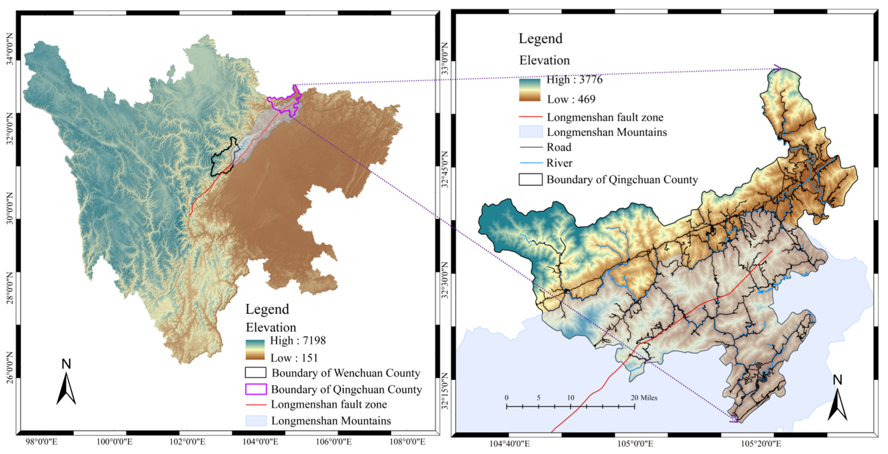
Wenchuan County, located between 31°43′10″ N to 30°45′37″ N latitude and 102°51′46″ E to 103°44′37″ E longitude, lies within the transitional zone between the eastern edge of the Qinghai-Tibet Plateau and the Sichuan Basin. It is situated at the junction of the Qionglai Mountains and the Longmen Mountain tectonic belt [17] (Figure 1). As a county under the jurisdiction of the Aba Tibetan and Qiang Autonomous Prefecture in Sichuan Province, Wenchuan covers an area of approximately 4084 km2. The region exhibits a typical high-mountain canyon topography, characterized by a stepped terrain descending from northwest to southeast. This results in significant elevation differences: the main peak of the Four Girls Mountain in the northwest reaches an altitude of 6250 m, whereas the lowest elevation at the outlet of the Min River in the southeast is only 780 m, producing a relative elevation difference of 5470 m.
The Minjiang River mainstem traverses the entire county for approximately 88 km, with tributaries such as the Zagunao River and Caopo River having carved deeply incised valleys [18]. Ribbon-shaped terraces and alluvial fans have developed along these rivers and constitute the primary economic activity zones in the region. The Wolong National Nature Reserve, located in the southwest, preserves well-developed Quaternary glacial landforms and pristine forest ecosystems, and has been recognized as a global biodiversity hotspot.
Geologically, the study area lies at the intersection of the Longmen Mountain Central Fault Zone (Yingxiu-Beichuan Fault) and the Houshan Fault (Wenchuan-Maoxian Fault). The region is strongly influenced by the eastward thrust of the Qinghai-Tibet Plateau, resulting in intense tectonic activity. Following the Ms 8.0 Wenchuan earthquake in 2008, the rock mass fragmentation index increased by 40–60%, leading to the formation of numerous landslide deposits.
The climate exhibits typical vertical zonation: the southern Xuankou-Yingxiu region receives an annual average precipitation of 1100–1332 mm, whereas the northern Weizhou-Miansi region receives only 528–700 mm. Approximately 70% of the precipitation is concentrated between June and September, with maximum hourly rainfall intensities reaching 56.7 mm. This precipitation pattern serves as a critical trigger for debris-flow events [19].
Ecologically, the region maintains a vegetation coverage rate of 48%, featuring a complete vertical zonation sequence ranging from subtropical evergreen broad-leaved forests to alpine meadows. Monitoring data from 2023 indicate that intact ecological chains remain, including top predators such as snow leopards. According to the latest statistics, the county has a population of 90,000 (as of 2023), with Qiang and Tibetan ethnic groups comprising 61% of the total, creating a distinctive multi-ethnic cultural landscape.
Overall, Wenchuan County’s unique terrain—characterized by abrupt topographic changes, an active tectonic background, and extreme precipitation patterns—interacts synergistically, making it an ideal setting for studying the cascading effects of geological disasters. These natural geographic features also provide a representative research context for subsequent studies on debris-flow susceptibility.

2.2. Selection of Conditioning Factors

The formation mechanism of debris-flow is highly complex, typically influenced by an interplay of factors, including topography, geology, environment, and human activities [7]. Terrain morphology and slope gradient are critical when controlling the accumulation of loose solid materials, which can retain substantial water volumes and create favorable conditions for rapid flow initiation. Complex geological structures—characterized by faults, folds, and weathered or fragmented rock masses—are particularly susceptible to debris-flow initiation [20]. Environmental conditions also play a direct and indirect role, primarily by affecting surface materials. Additionally, human activities serve as significant triggers; for example, excavation related to construction projects can destabilize slopes and release large quantities of loose material.
Susceptibility zonation of debris flows requires the analysis of diverse datasets to identify appropriate conditioning factors, making the selection of suitable factors a critical step. Based on debris-flow causative mechanisms and established studies [8], this research selected 19 conditioning factors across four categories—topography, geology, environment, and human activities—for susceptibility assessment in the study area. Topography, geology, and environmental conditions primarily govern debris-flow formation potential, while rainfall and human activities serve as the main triggering factors.
Specifically, the topographic factors (n = 11) include elevation, slope, slope aspect, profile curvature, plan curvature, compound curvature, topographic relief, terrain roughness index, topographic wetness index (TWI), stream power index (SPI), and sediment transport index (STI). Elevation data were obtained from Google Earth, while the other topographic variables were derived from a digital elevation model (DEM). The geological factors (n = 2) consist of strata and distance from the fault; strata data were sourced from the National Geological Data Center, and the distance from the fault was calculated based on the DEM. Environmental factors (n = 4) include the normalized difference vegetation index (NDVI), land cover, average annual rainfall, and distance from the river. These datasets were obtained from NASA, the China Meteorological Administration, and DEM-derived calculations, respectively. Human activity factors (n = 2) comprised distance from the road and POI kernel density. Distance from the road was indirectly derived from the DEM, while POI kernel density was calculated using Baidu POI data.
The selection of these 19 variables was grounded in their mechanistic relevance to debris-flow initiation. Topographic attributes directly influence hydrological and gravitational processes, geological structures govern slope stability and material strength, while environmental and anthropogenic factors affect surface disturbances and triggering conditions. The combined consideration of these factors enables a comprehensive characterization of the susceptibility environment. This selection was further informed by previous empirical studies and expert consultations to ensure both theoretical rigor and practical applicability.
Although incorporating a large number of conditioning factors will increase model dimensionality, it also facilitates capturing complex nonlinear interactions, especially when using tree-based models such as random forest. To address multicollinearity and ensure model stability, feature normalization and importance analysis were performed during the preprocessing and SHAP interpretation stages. The model evaluation results (AUC = 0.9931) further demonstrate the model’s capability to effectively handle high-dimensional input and confirm that the selected factor set positively contributes to prediction accuracy. Nonetheless, future research could explore dimensionality reduction or feature selection techniques to optimize computational efficiency without sacrificing performance.
The integration of these multidimensional factors provides a robust foundation for modeling debris-flow susceptibility.

3. Methods

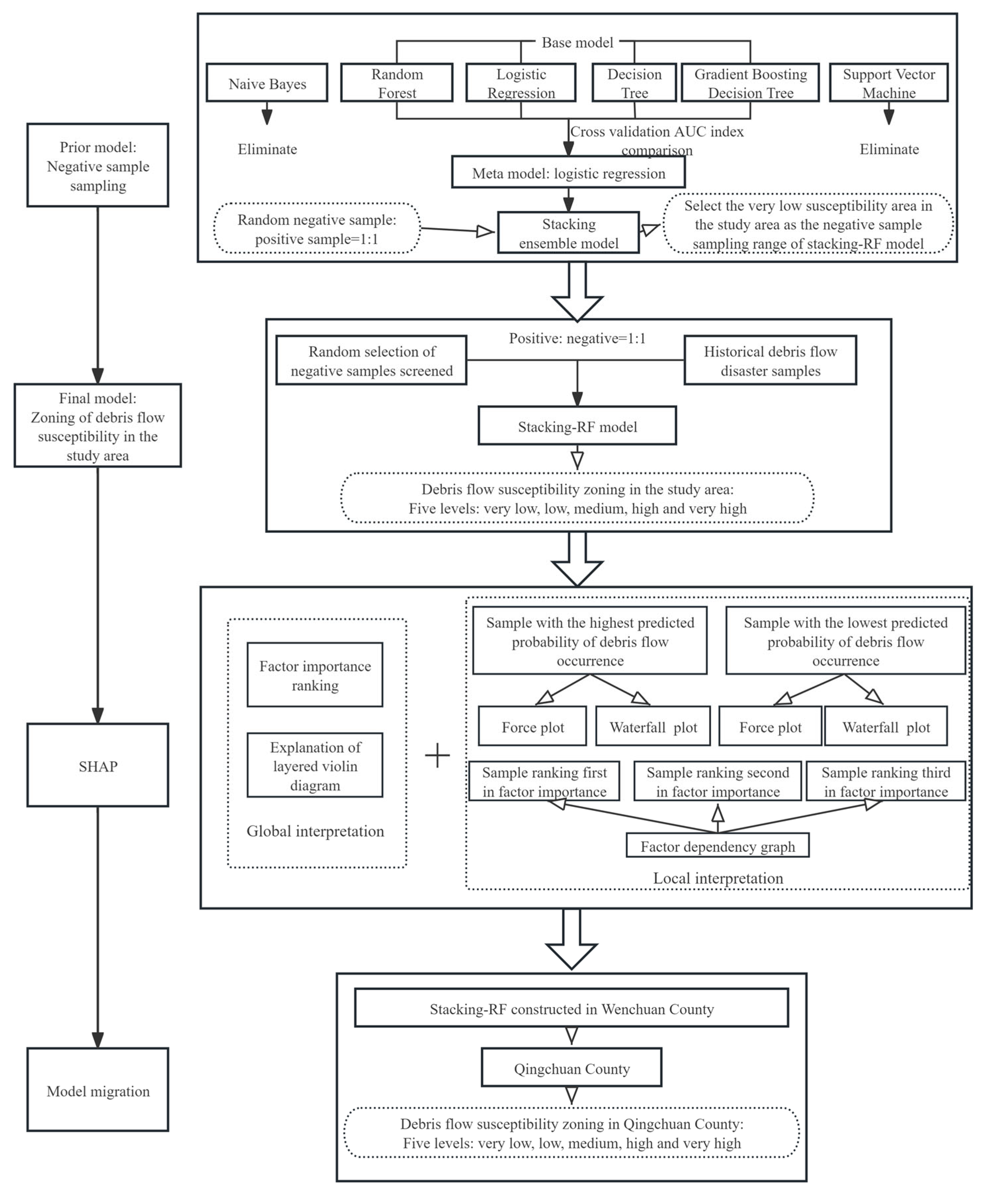
This study proposes a high-precision and interpretable debris-flow susceptibility assessment framework that integrates two-stage modeling and SHAP-based explainability. The framework includes four primary steps: (1) data construction, (2) negative sample screening via stacking ensemble learning, (3) posterior susceptibility prediction using a random forest model, and (4) interpretability analysis.
To enhance clarity, the overall process is summarized in a schematic flowchart (Figure 2), which visually presents the complete methodology, including data preparation, negative sample screening, model training, and an explanation of the results [21].

3.1. Negative Sample Screening via Stacking Ensemble Learning

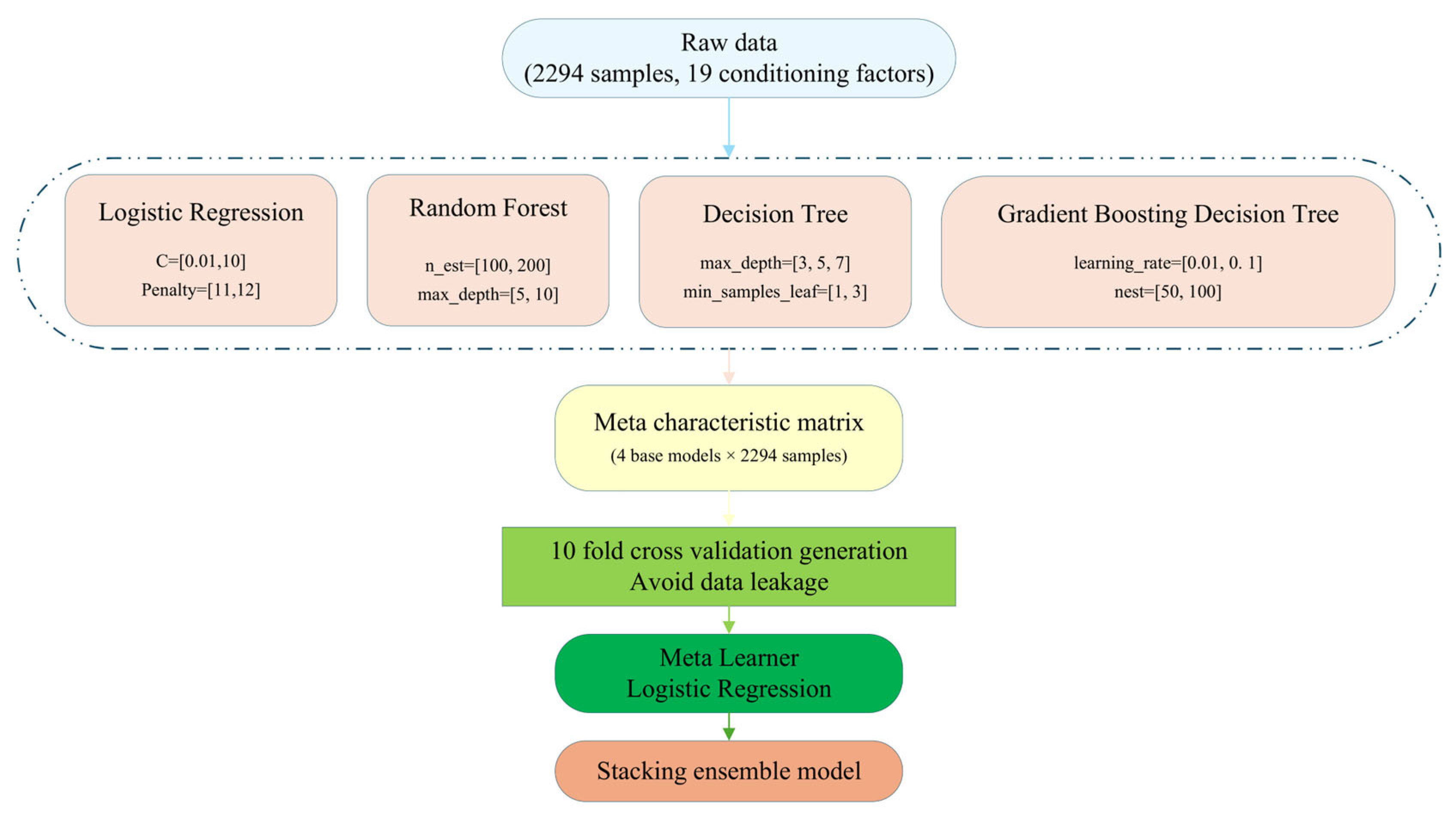
First, the study area was divided into 2294 watershed units using ArcGIS 10.8, and 19 conditioning factors (topographic, geological, environmental, and anthropogenic factors) were extracted to form the initial dataset. To mitigate pseudo-negative sample bias, a stacking ensemble model was applied to screen reliable negative samples.
The stacking model integrates four base learners—LR, RF, DT, and GBDT—with LR serving as the meta-learner [22,23,24,25]. Tenfold cross-validation was used to generate meta-features, and the final output susceptibility probabilities were classified using the Jenks natural breaks method [26]. Watershed units with very low predicted susceptibility and no recorded debris-flow history were selected as reliable negative samples. A balanced dataset (110 positive and 110 negative samples) was constructed for posterior modeling [27]. Stacking ensemble model architecture see Figure 3.
Although stacking improves model generalization, it requires relatively higher computational resources due to the repeated training of multiple base learners and cross-validation. In this study, all training and validation procedures were executed on a standard workstation (Intel Core i9-185H CPU, NVIDIA RTX 4060 GPU, 32 GB RAM), with total model training time remaining under 1.5 h, indicating its computational feasibility for practical applications.

3.2. Stacking-Random Forest Model

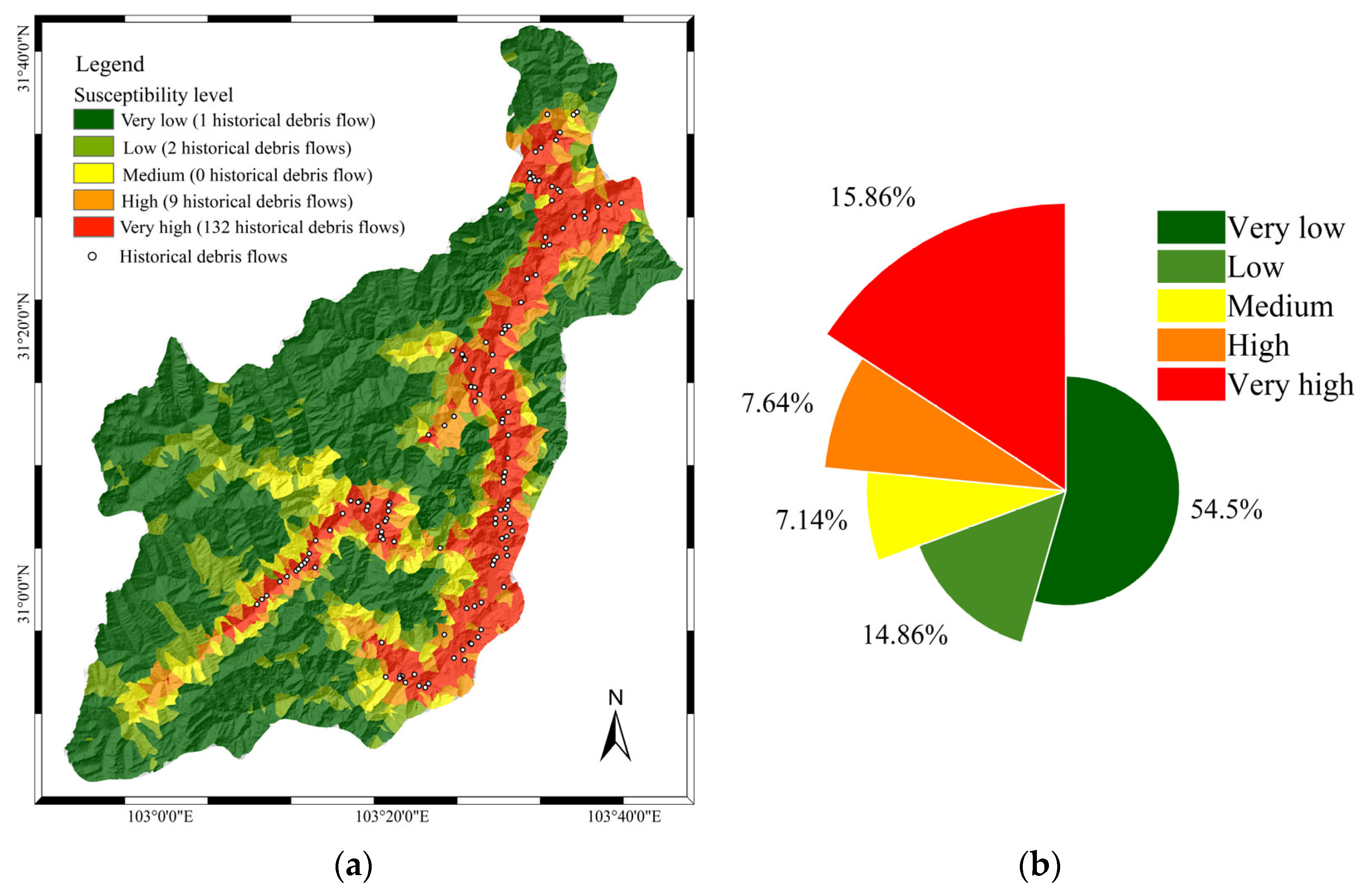
In the second stage, Stacking-RF was selected as the susceptibility prediction model for application in the research area [14], leveraging its mechanism of integrating multiple decision trees to enhance model stability and generalization capability. The Stacking-RF model was implemented via the Scikit-learn library, using the default hyperparameters. The input data comprised a stacking ensemble-optimized balanced sample set of 19 terrain, geological, environmental, and human activity factors. This dataset was partitioned through stratified random sampling into a 154-sample training set and a 66-sample test set [28]. Stratified 10-fold cross-validation was additionally applied to the training data to rigorously evaluate model stability and robustness across different data partitions [29]. The trained RF model was then used to predict susceptibility probabilities for the entire study area. The resulting probability raster was spatially visualized within the ArcGIS platform. Using the natural breaks method, the susceptibility probability raster was classified into five levels: very low, low, medium, high, and very high. The final susceptibility zonation map exhibited strong agreement with the spatial distribution of historical debris-flow events. Notably, the very high susceptibility zone encompassed 89.4% of the known debris-flow initiation sites, validating the model’s predictive reliability and spatial applicability.

3.3. Validation Metrics

Based on the binary confusion matrix, this paper selects accuracy, precision, recall, and F1-score as the validation metrics for the models. All four metrics range from (0, 1), and the formulas are as follows:
Accuracy   = TP + TN TP + FP + TN + FN
Precision = T P T P + F P
Recall = T P T P + F N
F 1 s c o r e = 2 P R P + R
where P denotes precision (Equation (2)) and R denotes recall (Equation (3)).
Model performance was assessed using standard classification metrics: accuracy, precision, recall, and F1-score, based on the confusion matrix. Additionally, receiver operating characteristic (ROC) curves and AUC values were used to evaluate prediction performance. High AUC scores (e.g., >0.99 for the posterior model) indicated strong discriminatory power [30].

3.4. SHAP Model Explanation

To enhance interpretability, SHAP was employed. SHAP assigns contribution scores to each feature for every prediction, based on cooperative game theory [31]. SHAP elucidates model predictions by quantifying the contribution of each input feature to the final output relative to a baseline expectation. For any individual prediction, SHAP values decompose the model’s decision into additive feature attributions, revealing how many factors, like slope angle, NDVI, or proximity to infrastructure, can locally increase or decrease the predicted susceptibility probability. Three levels of interpretation were completed:
  • Global explanation: Using SHAP summary plots to identify overall feature importance.
  • Local explanation: Applying force plots and waterfall charts to explain specific sample predictions.
  • Dependency analysis: Revealing nonlinear relationships and interactions through dependence plots, especially for top features like distance from roads or POI density.
SHAP explanations uncovered key insights into the physical mechanisms driving susceptibility and improved our understanding of the model’s decision logic, especially in high-risk zones.
Compared to traditional feature importance methods such as Gini impurity-based approaches, SHAP provides distinct advantages:
  • Theoretical foundation: SHAP values adhere to game theory axioms—efficiency, symmetry, dummy, and additivity—ensuring local accuracy and fairness.
  • Additive decomposition: SHAP decomposes any prediction into base value and feature contributions.
  • Model agnosticism: SHAP works with tree models, neural networks, and more, and is highly effective in revealing nonlinear interactions in random forests.

4. Results

4.1. Model Performance Comparison

4.1.1. Baseline Model Performance Evaluation

Table 1 summarizes the performance comparison of six machine learning models for debris-flow susceptibility prediction. Evaluation of the test set showed that the GBDT model achieved the best overall performance, with the highest AUC of 0.9035, recall rate of 0.9062, and accuracy of 0.8030, confirming its strong capability when identifying debris-flow-prone areas. The RF model exhibited comparable performance, achieving an AUC of 0.8952, although its accuracy was relatively lower at 0.7436. LR demonstrated stable performance, with an AUC of 0.8704, balanced recall of 0.8750, and an F1 score of 0.8235, indicating robust predictive ability. The DT model showed notable overfitting, with a training set AUC of 0.9936 but a decline to 0.8024 on the test set. Naïve Bayes (NB) analysis presented a characteristically high precision of 0.8889 but a low recall value of 0.5000, resulting in a reduced F1 score of 0.6400, likely reflecting the method’s limitations due to its independence assumptions. The SVM model performed the poorest, with an AUC of 0.6769 and a recall of only 0.2188, demonstrating limited capability in identifying debris-flow susceptible areas.
Model stability analysis revealed notable discrepancies between training and test performances in tree-based models (RF, GBDT, DT), indicating a limited generalization ability due to their high complexity. In particular, the AUC gap for the DT model reached as high as 0.1912. In contrast, LR exhibited only a minor AUC fluctuation of 0.0061, while NB surprisingly showed an AUC increase of 0.1530, both reflecting substantially smaller variations. Considering the trade-off between performance and diversity, this study selected GBDT, RF, LR, and DT as the base learners for the stacking ensemble model.

4.1.2. Performance Evaluation of the Stacking Ensemble Model and Stacking–Random Forest Model

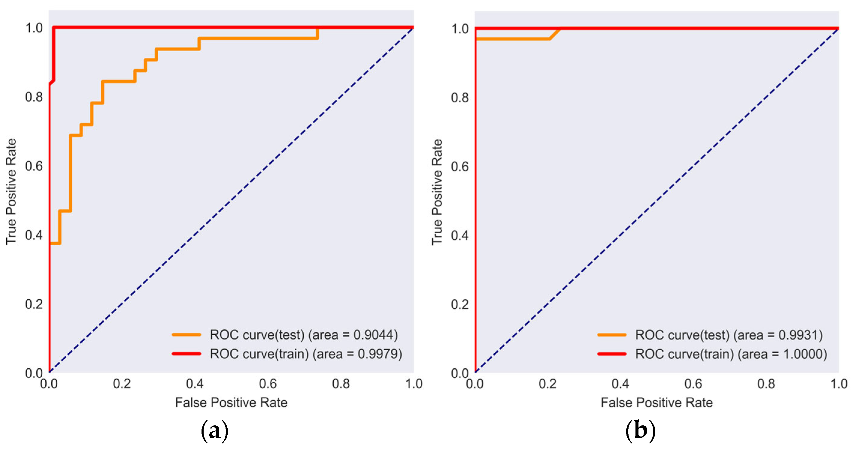
Table 2 summarizes the performance evaluation of the stacking ensemble model and the Stacking-RF model developed in this study, with their corresponding ROC curves presented in Figure 4. The stacking ensemble model demonstrated excellent performance on the training set, achieving an AUC of 0.9979 and an accuracy of 0.9805. Its ROC curve approached the theoretical optimum, indicating outstanding discriminatory capability. On the test set, the model maintained a stable performance, with an AUC of 0.9044, accuracy of 0.8182, a well-defined ROC curve, and most notably, a high recall of 0.8750.
The Stacking-RF model exhibited superior performance, achieving perfect scores on the training set with an AUC and accuracy of 1.0000. Most notably, it maintained excellent performance on the test set, attaining an AUC of 0.9931, accuracy of 0.9697, and a precision of 1.0000. Its ROC curve remained exceptionally close to the upper left corner of the graph, indicating outstanding discriminative capability.
As illustrated by the ROC curve comparison shown in Figure 4, the stacking ensemble model achieved a higher test-set AUC of 0.9044 than any of the six individual base models listed in Table 1. This confirms that the stacking ensemble approach, which leverages the combined predictive strengths of diverse base learners such as LR and Random Forest (RF), delivers more stable and reliable performance. Notably, its test-set recall of 0.8750 significantly exceeds that of other models, with SVM and NB achieving recalls of only 0.2188 and 0.5000, respectively. Furthermore, the visual comparison between Figure 4a and Figure 4b clearly demonstrates the enhanced capability of the ensemble strategy in identifying debris-flow-prone areas.
The outstanding performance of the Stacking-RF model, with its test-set AUC of 0.9931, further confirms that high-quality negative sample screening and optimization during model training substantially improve predictive accuracy.

4.2. Negative Sample Screening via Stacking Ensemble Model

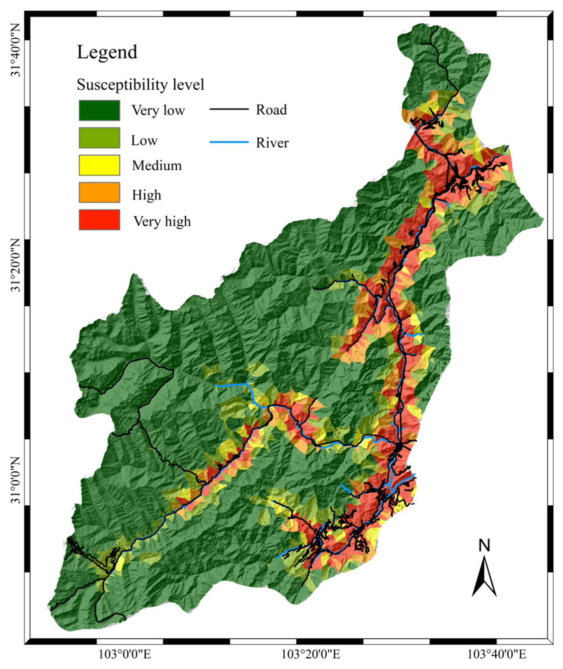
Based on the debris-flow susceptibility probability predictions generated by the stacking ensemble model for the entire study area, the region was classified into five susceptibility levels—very low, low, medium, high, and very high—using the natural breaks method in ArcGIS 10.8. The resulting debris-flow susceptibility zoning map is presented in Figure 5 and is hereafter referred to as the zoning map.
A comprehensive analysis of the negative sample screening results, specifically those areas identified as having very low susceptibility by the model, reveals strong consistency with the model’s predictive rationale. This validates the model’s effectiveness in excluding interfering samples and improving the overall classification accuracy. The following discussion focuses on two key aspects: the model’s negative sample screening mechanism and the geographical characteristics and validation of the screened negative samples that were classified as very low susceptibility zones.

4.2.1. Negative Sample Screening Mechanism

The stacking ensemble model significantly improves the distinction between high-noise areas—potentially misclassified as low risk—and genuinely low-risk zones by:
  • Integrating predictions from four base learners (random forest, logistic regression, decision tree, and gradient boosting decision tree).
  • Employing a multi-factor collaborative filtering mechanism through the dynamic adjustment of sample weights, guided by prior geological knowledge. This mechanism comprehensively analyzes all 19 conditioning factors, including strata, topographic relief, and distance from faults.
Areas selected as negative samples, specifically those classified as of very low susceptibility, consistently exhibit three key characteristics: stable geological conditions, minimal human activity impact, and low hydrological–climatic risk. Further analysis revealed that over 90% of these very low-susceptibility zones have high values for both distance from fault and distance from river metrics, demonstrating that the model effectively excludes tectonically active zones and those regions prone to hydrogeological erosion during the screening process.
Regarding the probability threshold optimization, regions classified as of very low susceptibility correspond to the predicted probabilities between 0.00 and 0.17. This low-probability range reflects the model’s lower confidence in these areas and embodies a conservative classification strategy that prioritizes minimizing false positives—that is, avoiding the misclassification of truly low-risk areas as higher-susceptibility zones.

4.2.2. Validation of Geographical Characteristics of Very Low-Susceptibility Zones

Spatial analysis of the zoning map reveals significant correlations between geographical attributes and the characteristics of those negative samples identified by the stacking ensemble model.
Geological and topographical stability analyses indicate that very low-susceptibility zones are primarily concentrated in ancient plateau regions or areas with extensive bedrock exposure, specifically those corresponding to old strata formations. These zones exhibit moderately low average topographic relief (52.30 m) and slope gradients (32.40°), which is consistent with the key screening criteria applied during negative sample selection, such as maintaining the topographic relief below 60 m.
The isolation effect of human activities is evident in the very low-susceptibility zones identified by the model, where all sampling units display substantial distances from roads. Spatial validation confirms these areas are remote from urban settlements and the major transportation corridors, as marked in Figure 5. This finding demonstrates the model’s high sensitivity to anthropogenic factors.
The coupled stabilizing influence of climate and vegetation is apparent in the very low-susceptibility zones. Despite the sparse vegetation cover indicated by NDVI values of around 0.1 and moderate average annual rainfall, ranging from 500 to 800 mm, grassland and forest remain the dominant land cover types. Soil stabilization through root system reinforcement partially mitigates the erosion potential. Crucially, the absence of high-probability debris-flow signals in these zones confirms the model’s ability to identify environmental stability via the vegetation–climate coupling effect.

4.3. Susceptibility Zonation Using the Stacking–Random Forest Model

The trained Stacking-RF model was applied to predict debris-flow susceptibility across the entire study area. The probability outputs were imported into ArcGIS, where the natural breaks (Jenks) method was used to generate the susceptibility zonation map (Figure 6). The study area was classified into five susceptibility levels: very low, low, medium, high, and very high.
Historical debris-flow initiation points (n = 143) show strong spatial correspondence with the zonation pattern, validating the model’s reliability. Figure 6 presents both the distribution of historical events and the proportional area of each susceptibility class.
The zonation results demonstrate significant spatial agreement with historical debris-flow occurrences. These outcomes provide robust scientific support for regional debris-flow prevention planning and enhanced risk management strategies.

4.4. Model Cross-Regional Validation in Qingchuan County

To evaluate the regional adaptability and generalization capability of the Stacking-RF model, Qingchuan County—which is geologically similar to Wenchuan County—was selected as an independent validation area. Situated in the northern segment of the Longmenshan Fault Zone, Qingchuan experienced comparable landslide deposits and tectonic disturbance intensity following the 2008 Wenchuan earthquake (Figure 7), providing a solid basis for comparative analysis.
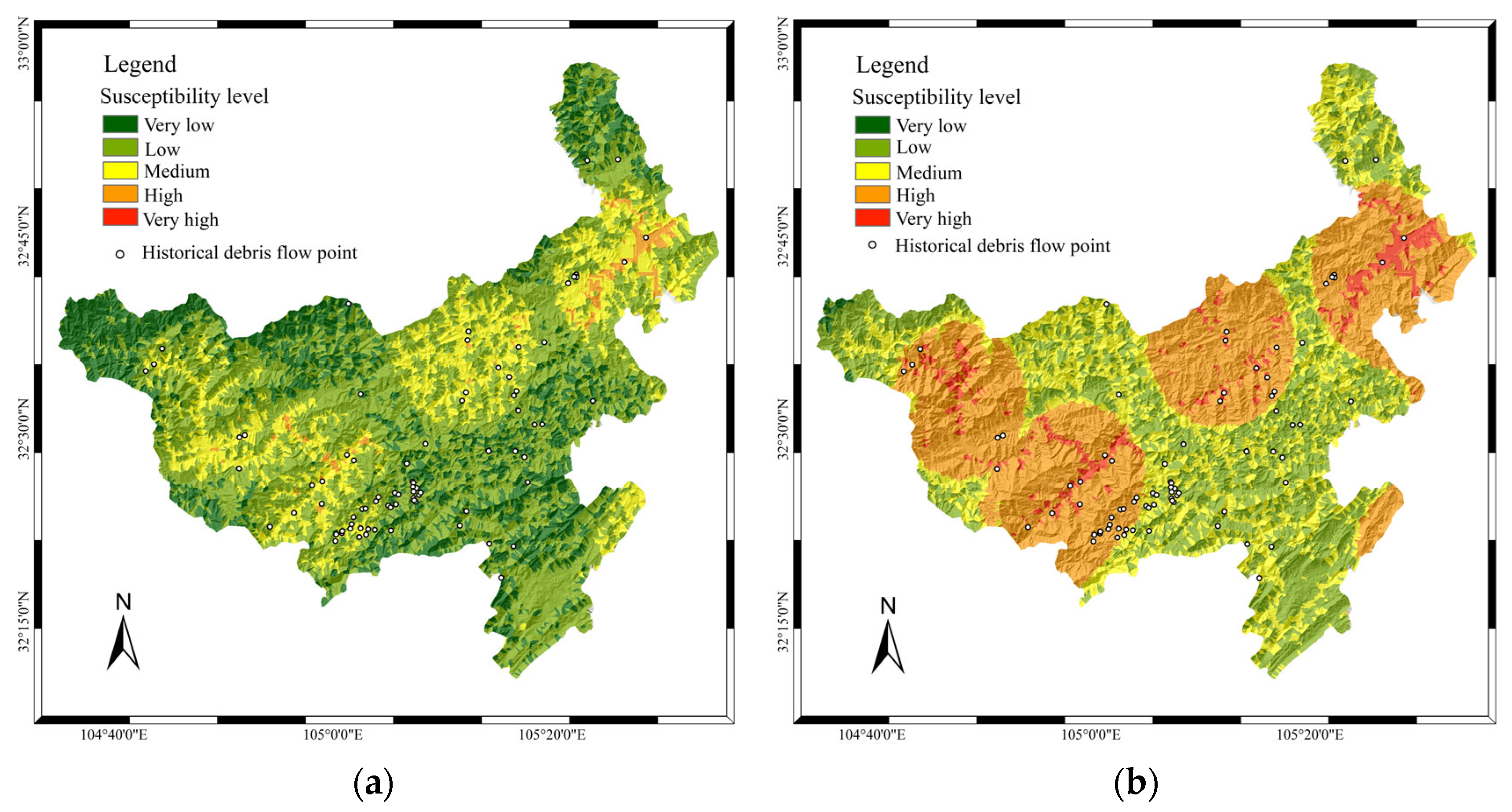
During model transfer, the same factor system and data processing workflow were applied. Nineteen conditioning factors, encompassing topography, geology, environment, and human activities, were extracted. The pre-trained Stacking-RF model was then used to predict debris-flow susceptibility across Qingchuan County, with its performance compared with a conventional random forest model.
Model outputs were classified into five susceptibility levels (from very low to very high) using ArcGIS’s equal interval method. Analysis of 88 historical debris-flow initiation points revealed:
(1)
Conventional RF model:
  • Over 70 percent of historical disasters occurred within zones classified as very low to low susceptibility, indicating high false positive rates;
  • Fewer than 5 percent of disasters were located in high- or very high-susceptibility zones, demonstrating severe underprediction;
  • Zero events in very high-susceptibility zones.
(2)
Stacking-RF model:
  • Disaster proportion reduced in very low- to low-susceptibility zones to 22.73%;
  • Elevated proportion in high- to very high-susceptibility zones to 53.41%;
  • Increased very high-susceptibility zone density from 0 to 0.0469 locations/km2.
The Stacking-RF model strategy reduced misclassification rates by at least 48 percent and false positives by approximately 48 percent in Qingchuan. This demonstrates superior spatial clustering and identification efficacy (Figure 8, Table 3). Conversely, conventional models showed weak spatial concordance with disaster distribution, underestimating the high-risk areas—validating the enhanced framework’s advantages in terms of regional generalization and spatial precision.

4.5. SHAP Explanation

4.5.1. Global Explanation

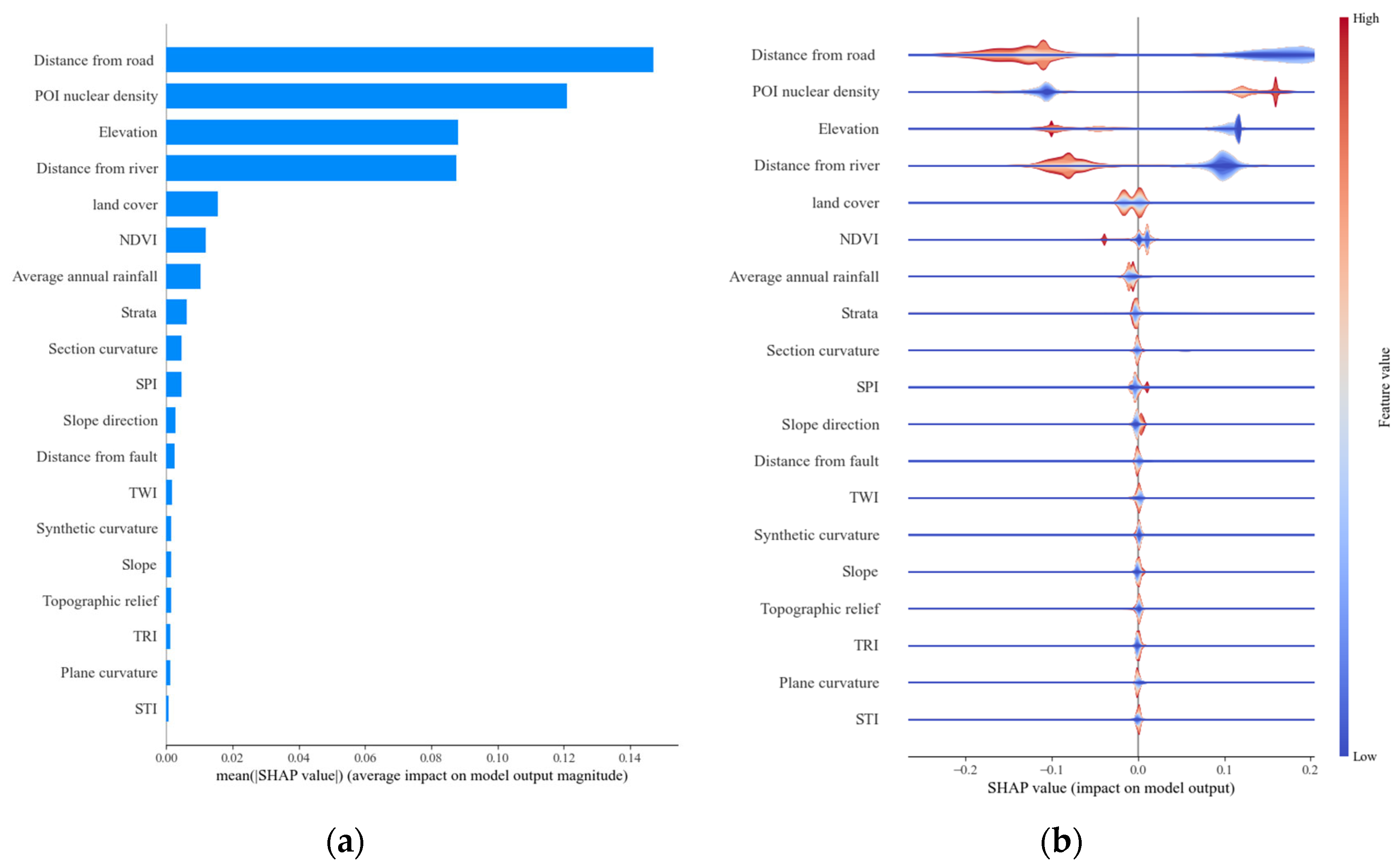
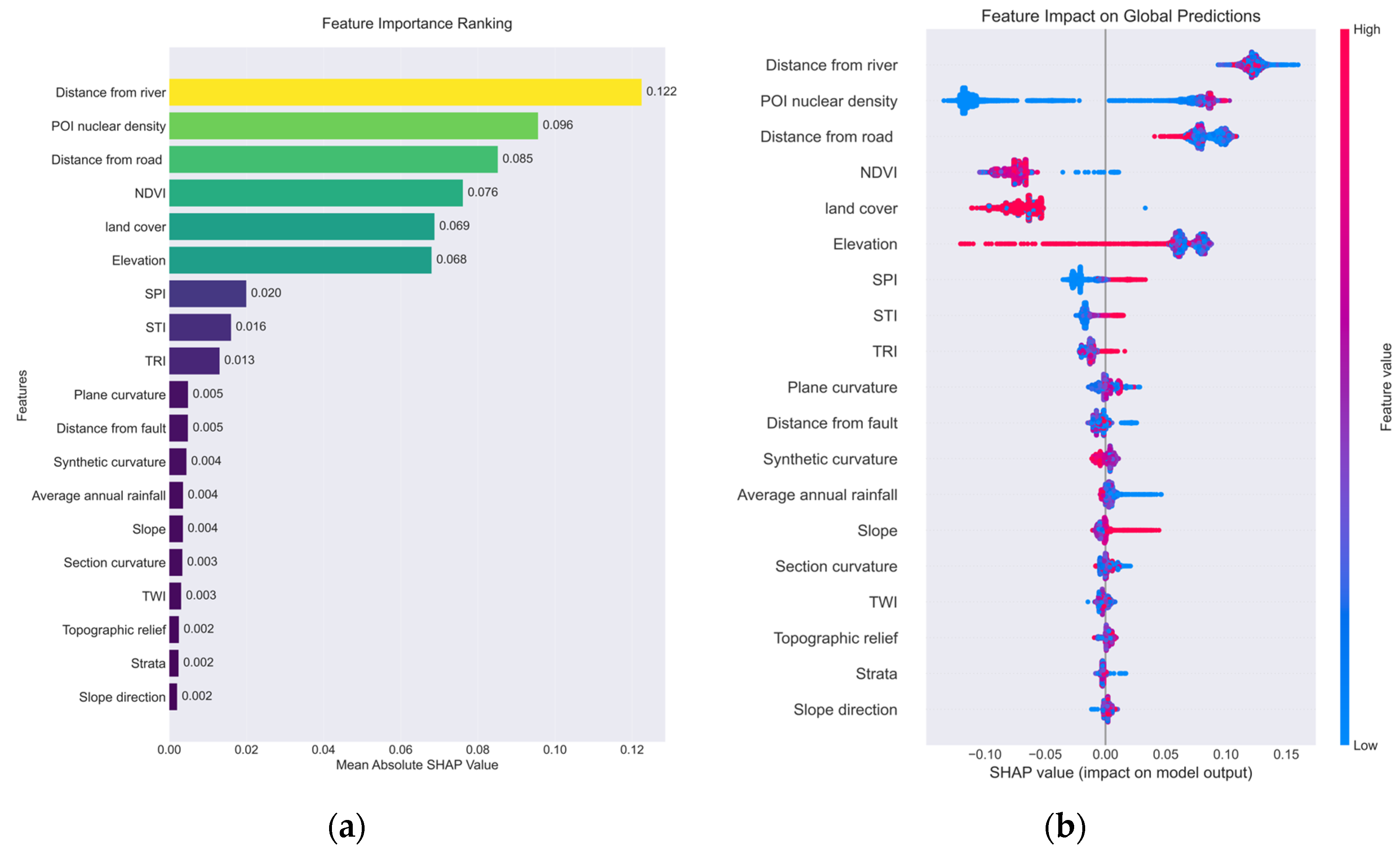
A global interpretability analysis of the random forest model using SHAP revealed the directionality and relative importance of input features on debris-flow susceptibility predictions (Figure 9). The results are visualized in two forms:
  • Feature importance ranking plot (ordered by descending mean |SHAP| value);
  • SHAP summary plot (depicting the distributional relationship between feature values and SHAP values).
Feature Importance Ranking
As demonstrated in Figure 9a, the distance from the road emerges as the most influential feature, with a mean absolute SHAP value of 0.15, reflecting the model’s high sensitivity to its variation. The second and third most significant features are POI kernel density and elevation, showing mean absolute SHAP values of 0.12 and 0.09, respectively. Distance from the river and land cover also demonstrated a substantial influence. Conversely, features such as plane curvature, TWI, and topographic relief exhibited mean absolute SHAP values below 0.02, signifying that they made negligible global contributions to model predictions.
Analysis of Feature Influence Direction and Patterns
The SHAP summary plot (Figure 9b) further elucidates the mechanisms by which key features influence prediction results.
(1)
Key linear features
Regarding the distance from the road, SHAP values predominantly cluster in the negative range—specifically, below zero—indicating an inverse linear relationship with predicted susceptibility. Critical analysis reveals that proximity to roads, represented by smaller feature values, correlates with stronger positive contributions to predictions of high susceptibility. This occurs because negative SHAP values signify model predictions exceeding the baseline susceptibility level.
For POI kernel density, SHAP values concentrate within the positive range—specifically, above zero—indicating a direct positive correlation with debris-flow susceptibility. Elevated POI kernel density significantly increases the probability of debris-flow occurrence.
(2)
Non-linear features
Elevation: SHAP values span both positive and negative ranges, revealing an inverted U-shaped relationship where low and high elevations exert negative influences with SHAP values below zero, while medium elevations significantly increase susceptibility, as evidenced by SHAP values above zero, indicating the existence of an optimal elevation range.
Slope: The scattered SHAP distribution implies context-dependent influence, with different slope ranges exerting positive or negative effects on susceptibility.
Land cover: Dispersed SHAP values reflect distinct positive or negative contributions made by specific cover types, such as forest and bare ground, to susceptibility predictions.
(3)
Secondary features
Secondary features include annual average rainfall, distance from a fault, and NDVI display SHAP values oscillating near zero, with absolute magnitudes approximating zero. This suggests that their influence primarily depends on interactions with other features while contributing minimally overall. Hydrological-topographic indices, such as stream power index (SPI) and sediment transport index (STI), exhibit tightly clustered SHAP distributions featuring negligible absolute values, which is consistent with their low importance rankings.

4.5.2. Local Explanation

Local explanation of model predictions was conducted using SHAP force plots, waterfall plots, and dependence plots, revealing the decision logic of key samples and the nonlinear interaction mechanisms of key factors.
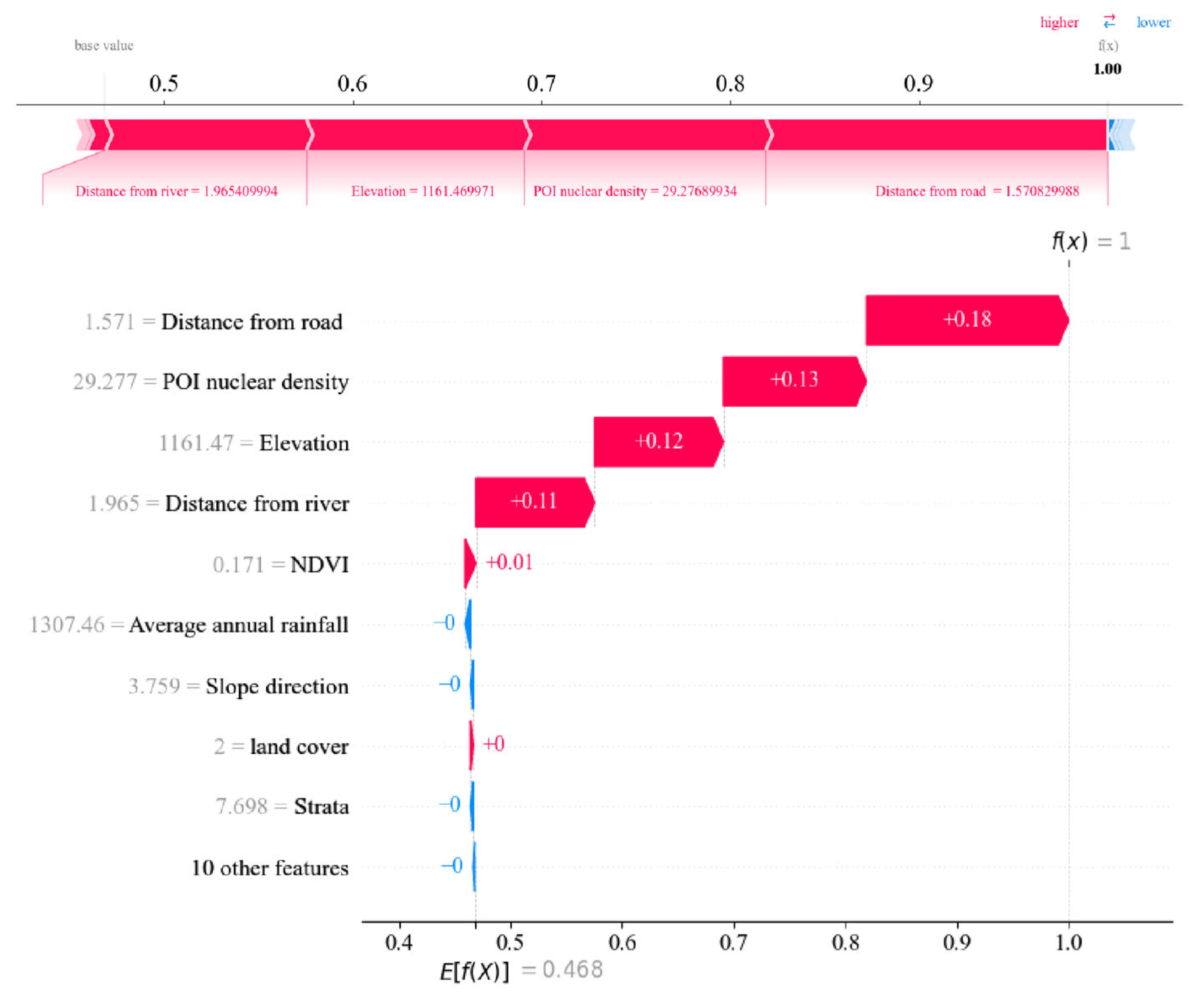
(1) The driving mechanism of the sample with the highest predicted probability of debris-flow occurrence is shown in Figure 10.
Key factor contribution: Distance from the road = 785 m, with a SHAP value of +0.18, serves as the core positive driving force (accounting for 32.7% of the total feature contribution), indicating that road proximity significantly increases the predicted probability of debris-flow occurrence.
Prediction value comparison: The sample prediction value (f(x) = 0.468 + ∑SHAP) is significantly higher than the population benchmark value E[f(X)] = 0.468, primarily due to the synergistic enhancement effect of road proximity and human activity density.
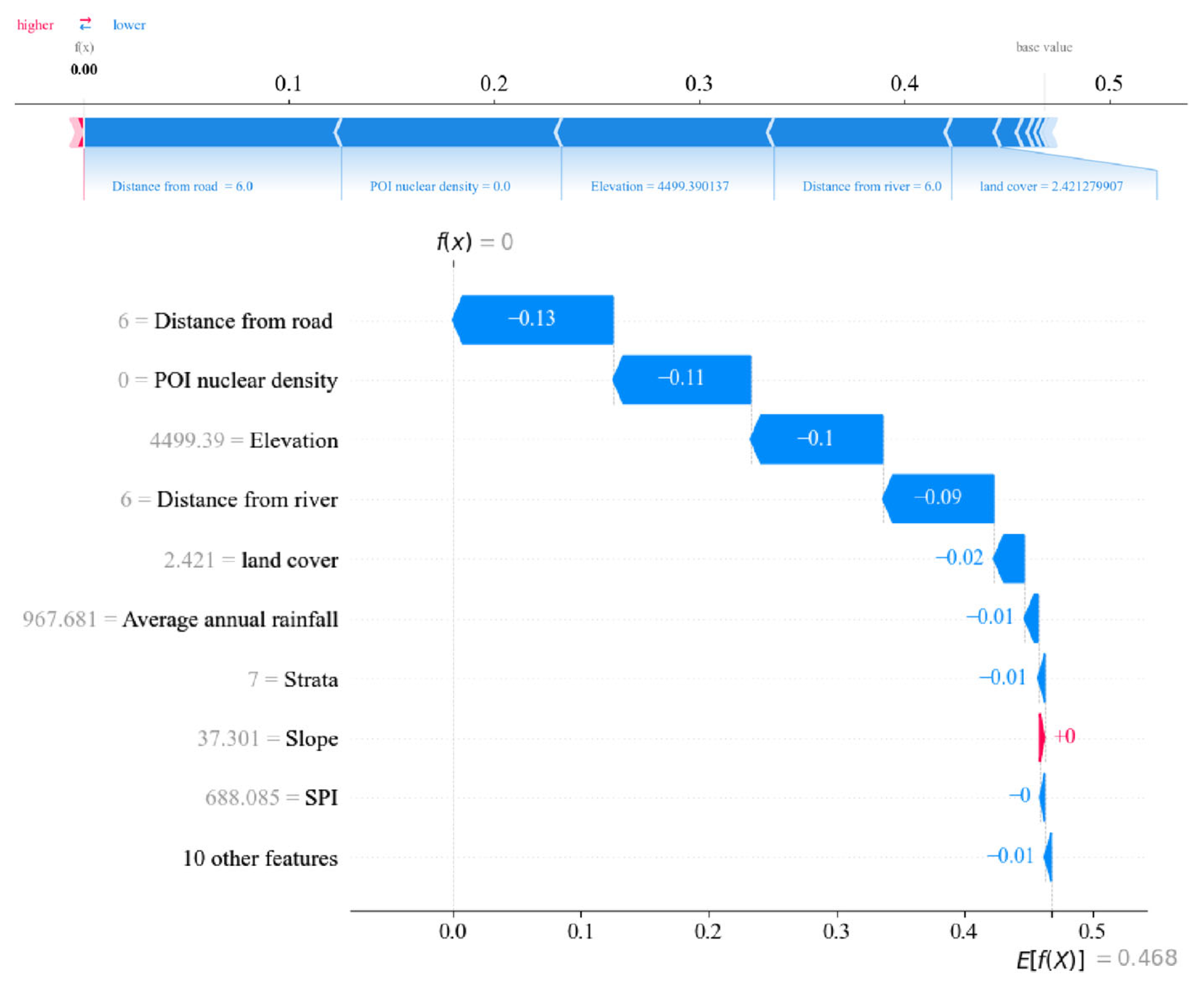
(2) The suppression mechanism of samples with the lowest predicted probability of debris-flow occurrence is shown in Figure 11.
Systematic negative contributions: The SHAP values for the distance from the road at >2500 m, POI kernel density = 0, and elevation = 4499.39 m were −0.13, −0.11, and −0.10, respectively (accounting for 79.4% of the total negative contribution), reflecting the significant suppression of predicted values by extreme spatial isolation (zero POI kernel density) and very high-altitude terrain.
Environmental factor reinforcement effect: The weak negative contributions of annual average precipitation (SHAP = −0.01) and geological age further reinforce the low-risk assessment.
(3) Nonlinear patterns of conditioning factor dependency.
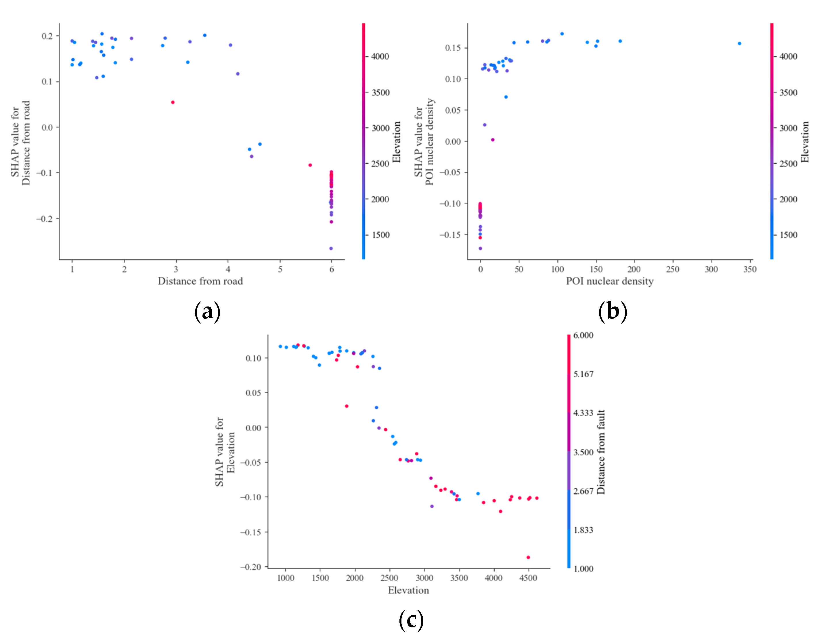
To analyze the contribution mechanism of key factors to single-sample predictions, this study analyzed the top three features, ranked by importance based on SHAP dependency plots.
(1)
Distance from the road (Figure 12a)
Within the mid- to low-altitude zone, below 2500 m, significantly positive SHAP values, as specifically observed in the blue data clusters, indicate that proximity to roads enhances debris-flow probability. Conversely, in high-altitude zones above 3500 m, the SHAP values consistently approach zero, as seen in the pink clusters, demonstrating the limited effectiveness of infrastructure interventions in such terrains.
(2)
POI kernel density (Figure 12b)
Threshold effect analysis revealed significantly positive SHAP values when POI kernel density exceeded 50, confirming that human activity density positively influences risk prediction outcomes. Regarding the spatial distribution constraints, samples with high POI kernel density exceeding 50 are concentrated predominantly in low- to mid-altitude ranges, visually identifiable as blue-purple data points. This pattern indicates the model’s dependency on human activity intensity, specifically within lower elevation areas, using this element for risk assessment.
(3)
Elevation (Figure 12c)
A monotonic decreasing relationship exists between elevation and SHAP values, which is characterized by positive contributions from areas below 2000 m in elevation and negative contributions from regions exceeding 3000 m in elevation.
Modulating effect of fault distance: In areas that are closer to faults (blue points), the rate of decrease in SHAP values for high-altitude samples slows down, revealing a threshold buffering mechanism where fault proximity mitigates the inhibitory effect of elevation.

4.5.3. Cross-Regional Mechanism Stability Validation: Qingchuan

To examine whether the factor-driven mechanisms remain consistent across regions, an interpretability analysis was performed on Qingchuan County’s predictions, as shown in Figure 13 and Figure 14.
Global explanation results (Figure 13) demonstrate that:
  • Factor importance rankings and SHAP summary plots in Qingchuan County align closely with those of Wenchuan County.
  • The top six features exhibit particularly high consistency.
  • The distributions of factors such as distance from the road and POI kernel density further corroborate the universal principle: “Human activity intensity dominates debris-flow risk.”
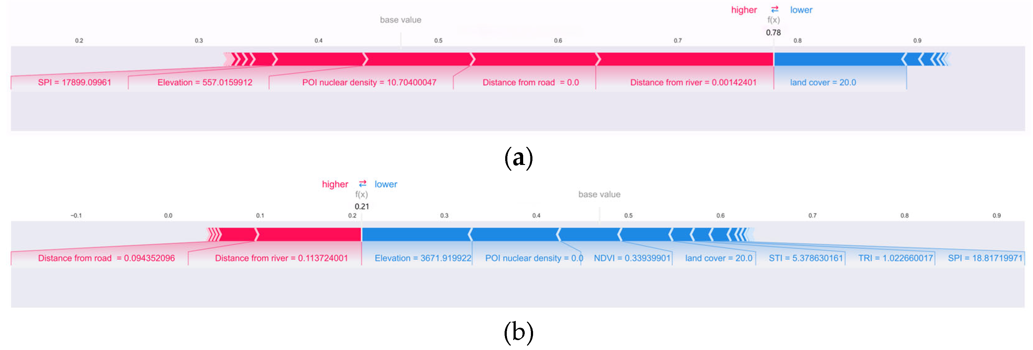
Local explanation results (Figure 14) reveal that:
  • Samples with the highest predictions are primarily driven by features like the distance from the road = 0 and distance from the river ≈ 0, collectively elevating the model’s high-risk probability assessment.
  • Conversely, samples with the lowest predictions display numerous features, including elevation = 3671.92 m and POI kernel density = 0, exerting an overall negative contribution to debris-flow prediction and thereby substantially suppressing the output probabilities.
  • Marked contrasts in the key factor values validate the model’s sensitivity to risk-level transitions between engineering-disturbed zones and sparsely populated areas, confirming the stability and transferability of feature threshold effects across regions.
These validation results robustly confirm that the Stacking-RF model exhibits exceptional transferability and stability:
  • The negative sample strategy derived from ensemble learning establishes a more reliable modeling foundation for new regions, significantly improving high-susceptibility zone identification.
  • The human activity–terrain environment synergy mechanism remains highly consistent across the regions, reflecting the model’s profound capability to characterize geological disaster formation.
This section demonstrates that the model possesses not only high predictive accuracy but also distinct spatial adaptability, making it generalizable to debris-flow prediction and spatial planning in other seismically active mountainous regions.

5. Discussion

This study establishes a debris-flow susceptibility assessment framework integrating data cleansing, model optimization, and mechanistic interpretation. The framework utilizes a stacking ensemble model to filter the high-reliability negative samples, employs a random forest model for high-precision prediction, and applies SHAP technology for mechanism elucidation. It systematically addresses two key limitations of conventional approaches—negative sample selection bias and limited model interpretability—offering a novel paradigm for geological hazard risk assessment. The discussion is organized around four main aspects: methodological innovation, mechanistic insights, uncertainties, and practical implications.

5.1. Methodological Innovation: Integrated Negative Sample Screening Enhances Model Generalization

The proposed stacking ensemble negative sample screening strategy effectively reduces the model bias arising from potentially unstable areas, as commonly encountered in traditional random sampling, such as with unrecorded disaster-prone steep slopes. By focusing on geologically consistent negative samples drawn from very low-susceptibility zones, this approach significantly improves the sample quality. As shown in Figure 5, the screened areas cluster within geologically stable highland bedrock zones with minimal human activity. These regions consistently exhibit maximum-range values for both fault distance and river distance, aligning closely with those characteristics of stable zones identified through field surveys [32].
This strategy elevated the posterior random forest model’s test-set performance to an AUC of 0.9931, with recall reaching 0.9375, markedly outperforming both the standalone random forest model (AUC = 0.8952) and the stacking ensemble model itself (AUC = 0.9044). These findings validate the efficacy of multi-model collaborative noise-filtering processes and highlight the critical impact of negative sample quality on model performance. In contrast to conventional methods, where sample heterogeneity previously caused an approximately 8% AUC reduction in Beichuan County’s global model [33], this framework quantifies regional stability via ensemble learning, providing a robust pathway for acquiring high-reliability negative samples during geological hazard assessment.
Compared with traditional susceptibility modeling methods that typically rely on single classifiers, our approach significantly improves model generalization by integrating negative sample screening and stacking ensemble learning. While earlier methods often struggle with imbalanced training data and overfitting issues, the proposed workflow achieves a more robust performance across multiple evaluation metrics. The combination of representative negative sampling and model fusion contributes to superior predictive accuracy, particularly in complex terrain scenarios, where traditional models tend to fail.

5.2. Mechanistic Analysis: Nonlinear Coupling Mechanisms of Human Activities and Topography

Through SHAP-based global and local interpretability analyses, the model demonstrated pronounced sensitivity to human activity factors, with distance from the road and POI kernel density emerging as primary drivers of debris-flow susceptibility. SHAP dependence plots reveal distinct thresholds: SHAP values increase markedly when the distance from the road is within 500 m and when POI kernel density exceeds 50 units/km2, indicating clear risk-sensitive thresholds. In high-altitude areas above 3000 m with sparse POI kernel density, these features contribute negatively, underscoring the regulatory influence of human activities on local risk distribution.
Elevation values exhibit a complex nonlinear pattern, with peak susceptibility observed between 1000 and 3000 m, while both lower and higher elevations correspond to reduced predicted probabilities. This trend is further modulated by proximity to fault lines, which mediates the elevation effects; for example, closeness to high-altitude faults mitigates reductions in SHAP values.
These observations are consistent with known geological mechanisms: road construction and human settlements enhance soil erosion and surface runoff, whereas human disturbances tend to reduce risk in high-altitude, resource-scarce zones. The influence of fault proximity partially offsets elevation-related prediction biases. Overall, this study not only advances methodological innovation but also enriches our mechanistic understanding of the nonlinear coupling between multiple factors.
The dominant influence of elevation, rainfall, and road proximity on debris-flow susceptibility aligns with commonly observed hazard patterns in mountainous areas. However, our analysis further reveals the nonlinear interactions among these variables—especially on how terrain curvature intensifies susceptibility under high rainfall conditions. Such compound effects were rarely captured in earlier studies based on linear assumptions or coarse factor discretization, highlighting the added value of using interpretable machine learning in mechanism exploration.

5.3. Uncertainty: Boundary Ambiguity and Dynamic Factor Deficiencies

Despite achieving high overall accuracy, the final random forest results exhibit classification uncertainty regarding approximately 12.3 percent of low-susceptibility zone samples. This primarily stems from two limitations:
  • A notable source of uncertainty stems from model ambiguity near the critical thresholds, particularly where NDVI values approach 0.1—indicating sparse vegetation—and when slope angles approximate 35°, which is commonly recognized as a geomorphic instability threshold. Under these conditions, the model demonstrates inconsistent prediction confidence, which is likely due to complex nonlinear interactions and overlapping susceptibility characteristics. While SHAP analysis reveals the sensitivity of predictions in such regions, it does not resolve classification ambiguity. Future improvements could involve integrating NDVI time-series datasets to better reflect seasonal vegetation variability, or implementing fuzzy classification and hybrid threshold-based models to address boundary uncertainty and improve decision-making clarity.
  • Static data constraints weaken the model’s temporal predictive capability by excluding dynamic factors such as hourly rainfall peaks, seasonal vegetation fluctuations, and slope deformation trends. These missing dynamics reduce the model’s responsiveness to event-based triggers (e.g., > 50 mm/h of rainfall) or temporal slope instabilities. Future work should consider integrating satellite-based InSAR deformation time series and TRMM/GPM rainfall datasets to model the short-term triggering mechanisms. Additionally, multi-temporal NDVI products can enhance the characterization of vegetation dynamics. Temporal sequence modeling techniques, such as attention-based LSTM or Transformer frameworks, will be explored to incorporate these dynamic factors and improve the model’s sensitivity to time-varying debris-flow triggers.
Furthermore, the model’s reliance on historical static data poses challenges in accounting for future climate change impacts. Rainfall, as a key triggering factor for debris-flow events, is projected to exhibit increasing variability in terms of intensity and distribution under evolving climatic conditions. The current framework does not capture such temporal dynamics, which may limit its predictive reliability in non-stationary environments. To address this issue, future improvements should incorporate dynamic or scenario-based data inputs, such as projected precipitation values from CMIP6 models, multi-temporal NDVI datasets, or hydrological outputs from climate-integrated models. Additionally, to ensure its long-term applicability, the model should undergo periodic recalibration using updated environmental indicators, including time-series NDVI, rainfall trends, and anthropogenic development indices. The integration of adaptive learning mechanisms or semi-automated retraining workflows would help maintain prediction accuracy as climate and land-use patterns continue to evolve.
The performance gap between the Stacking-RF model and baseline classifiers such as SVM and NB underscores the limitations of linear or shallow models for capturing complex spatial patterns. Traditional approaches often prioritize overall accuracy but lack the ability to explain localized misclassifications. In contrast, our model not only delivers higher predictive scores but also supports post hoc interpretability, enabling a deeper understanding of model behavior and spatial uncertainty.

5.4. Practical Implications: Precision Mitigation and Spatial Planning

Our findings provide actionable strategies for post-earthquake risk management:
  • Delineate priority avoidance zones encompassing 500-meter buffer zones along roads and medium- to low-altitude areas where POI kernel density exceeds 50 units/km2.
  • Enhance engineering standards to require slope reinforcement along roads that have been designed to withstand rainfall events, with a 50-year return period.
  • Enforce development restrictions in very high-susceptibility zones, which cover 15.86% of the study area and account for 92.3% of historical debris-flow events, through residential construction bans and the relocation of populations to low-susceptibility areas, characterized by topographic relief below 60 m.
Quantitative thresholds derived from SHAP analysis—especially the safety threshold of POI kernel density set below 50 units/km2—can be directly applied to regulate land development intensity. This explainability-to-policy framework effectively bridges the gap between technical model outputs and stakeholder decision-making, enabling science-based community disaster risk management.

5.5. Model Selection and Performance Divergence: Mechanistic Interpretations of Predictive Discrepancies

As shown in Table 1 and Figure 4, the predictive performance of different machine learning models exhibits significant variation. Specifically, ensemble-based models such as RF and GBDT achieved exceptionally high AUC values, with cross-validation results approaching 100%, while simpler models such as LR and NB performed notably more poorly, with AUCs below 75%.
This performance gap can be attributed to the inherent differences in model learning mechanisms. RF and GBDT are tree-based ensemble algorithms that are capable of capturing complex nonlinear relationships, feature interactions, and high-order decision boundaries. When applied to a relatively small, well-balanced, and noise-reduced dataset (110 positive and 110 negative samples), these models can fit the data with high precision during cross-validation. In contrast, LR and NB models rely on linear assumptions or conditional independence between features, which limits their ability to model the complex spatial and environmental factors influencing debris-flow susceptibility.
Additionally, the high performance of RF and GBDT does not necessarily indicate overfitting, as all models were evaluated using stratified 10-fold cross-validation, which effectively mitigates overfitting risk and ensures robustness across different data splits. The model’s generalizability was further tested by applying the trained Stacking-RF model to a neighboring region (Qingchuan County), where it still yielded consistent and reasonable susceptibility predictions.
These findings highlight the importance of selecting appropriate modeling frameworks that align with the complexity of the task. While simpler models offer greater interpretability, advanced ensemble methods provide superior predictive capability in nonlinear, multi-factor geospatial applications such as debris-flow susceptibility mapping.

5.6. Future Work: Toward Robust Validation and Field Integration

While the current study demonstrates high predictive accuracy and model interpretability, based on the available remote sensing and historical disaster datasets, field validation remains a critical next step to enhance the credibility of the results. In future studies, we plan to incorporate on-site investigation data, including actual debris-flow boundaries, soil composition, and hydrological measurements, to cross-check the model predictions in high-risk zones. Moreover, we aim to collaborate with local agencies to validate predicted hotspots using GPS-based field surveys and post-disaster reports.
To address the temporal dynamics, future work will also explore time-series model validation, particularly in those areas where multi-year monitoring data are available. This will help distinguish between transient and persistent susceptibility patterns. Ultimately, the integration of field-based evidence will allow for more reliable policy recommendations and risk mitigation strategies, ensuring that the model is both scientifically sound and practically actionable.

6. Conclusions

This study addresses two critical challenges in traditional debris-flow susceptibility modeling—namely, negative sample selection bias and insufficient model interpretability. By integrating stacking ensemble-based negative sample screening with a Stacking-RF model and SHAP-based interpretation, we proposed a predictive framework and applied it to Wenchuan County, Sichuan Province. The key findings are summarized as follows:
(1)
Negative sample screening significantly improves model generalization and reliability.
The initial stacking ensemble model (comprising LR, RF, DT, and GBDT) achieved a test-set AUC of 0.9044. By introducing a probability-based thresholding strategy to select highly stable zones as negative samples, we effectively eliminated pseudo-negative samples. This led to a well-balanced training dataset (1:1 ratio), enhancing the performance of the posterior RF model, which achieved a test-set AUC of 0.9931—an improvement of nearly 10% over the baseline RF model (AUC = 0.8952).
(2)
The Stacking-RF model enables high-precision early-warning and cross-regional applicability.
The optimized RF model demonstrated a recall of 0.9375 and a precision of 1.000. Spatial zoning revealed that 92.3% of historical disaster points were concentrated within the predicted very high-risk zones (covering only 15.86% of the study area). The model also generalized well to Qingchuan County, maintaining low false positive and false negative rates, confirming its practical potential for regional disaster prevention.
(3)
Human activity factors are dominant in the nonlinear driving mechanism of debris flows.
SHAP analysis revealed that distance from the road (0.15), POI kernel density (0.12), and elevation (0.09) were the top contributors. Risk sharply increased when the distance from the road dropped below 500 m or when the POI kernel density exceeded 50 units. Moreover, terrain factors interacted nonlinearly: elevation peaked in terms of risk between 1000 and 3000 m, while fault proximity (<1000 m) buffered the inhibitory effect of high altitudes (>3000 m), slowing the SHAP value decline by 37%.
This framework offers a high-precision, interpretable tool for debris-flow susceptibility assessment. Its combined innovations—negative sample screening, model fusion, and SHAP interpretability—can directly support spatial resilience planning and disaster mitigation in mountainous regions.
While the proposed framework demonstrates strong performance, its validation remains primarily model-based. Future research will incorporate field survey data to further validate prediction accuracy and the temporal dynamics of hazard evolution. In addition, expanding the model to multi-temporal datasets and other geographic regions may enhance its robustness and generalizability.

Author Contributions

Conceptualization, J.Z.; data curation, J.L.; formal analysis, J.Y.; investigation, J.L.; methodology, J.Z.; supervision, J.Z.; validation, J.L., H.W. and Y.C.; writing—original draft, J.L.; writing—review and editing, J.Z. and H.W. All authors have read and agreed to the published version of the manuscript.

Funding

This research was funded by the National Key Research and Development Program of China (2023YFC3007203).

Data Availability Statement

Data will be made available on request.

Conflicts of Interest

The authors declare no conflicts of interest.

Abbreviations

The following abbreviations are used in this manuscript:
SHAPShapley Additive Explanations
LRLogistic Regression
DTDecision Tree
GBDTGradient Boosting Decision Tree
RFRandom Forests
Stacking-RFStacking–Random Forest
SVMSupport Vector Machine
NBNaïve Bayes
ROCReceiver Operating Characteristic
AUCArea Under the ROC Curve
DEMDigital Elevation Model
TWITopographic Wetness Index
NDVINormalized Difference Vegetation Index
STISediment Transport Index
SPIStream Power Index
InSARInterferometric Synthetic Aperture Radar
TRMMTraining Resource Management Meeting

References

  1. Iverson, R.M. The physics of debris-flow. Rev. Geophys. 1997, 35, 245–296. [Google Scholar] [CrossRef]
  2. Yang, S.; Mei, G.; Zhang, Y. Susceptibility analysis of glacier debris flow by investigating glacier changes based on remote sensing imagery and deep learning: A case study. Nat. Hazards Res. 2023, 4, 539–549. [Google Scholar] [CrossRef]
  3. Cui, P.; Wei, F.Q.; He, S.M.; You, Y.; Chen, X.Q.; Li, Z.L.; Dang, C.; Yang, C.L. Mountain disasters induced by the 5 · 12 Wenchuan earthquake and disaster reduction measures. J. Mt. Sci. 2008, 26, 280–282. (In Chinese) [Google Scholar] [CrossRef]
  4. Wang, G.F.; Yang, Q.; Tian, Y.T.; Ye, Z.N.; Chen, Z.L.; Gao, Y.L.; Guo, N.; Deng, B. Construction of debris flow susceptibility evaluation model: A case study of Yangtang River section in Shimen Township, Bailong River Basin. Arid Zone Res. 2019, 36, 761–770. (In Chinese) [Google Scholar] [CrossRef]
  5. Sun, B.; Zhu, C.B.; Kang, X.B.; Ye, L.; Liu, Y. Susceptibility assessment of debris flow in Dongchuan, Yunnan based on information value model. Chin. J. Geol. Hazard Control 2022, 33, 119–127. (In Chinese) [Google Scholar] [CrossRef]
  6. Hong, H.; Liu, J.; Zhu, A.X.; Shahabi, H.; Pham, B.T.; Chen, W.; Pradhan, B.; Bui, D.T. A novel hybrid integration model using support vector machines and random subspace for weather-triggered landslide susceptibility assessment in the Wuning area (China). Environ. Earth Sci. 2017, 76, 652. [Google Scholar] [CrossRef]
  7. Perov, V.; Chernomorets, S.; Budarina, O.; Savernyuk, E.; Leontyeva, T. Debris flow hazards for mountain regions of Russia: Regional features and key events. Nat. Hazards 2017, 88, 199–235. [Google Scholar] [CrossRef]
  8. Zhou, X.; Wen, H.; Zhang, Y.; Xu, J.; Zhang, W. Landslide susceptibility mapping using hybrid random forest with GeoDetector and RFE for factor optimization. Geosci. Front. 2021, 12, 101211. [Google Scholar] [CrossRef]
  9. Zhang, K.; Sang, G.; Cheng, J.; Liu, Z.; Zhang, Y. Negative sampling strategy based on multi-hop neighbors for graph representation learning. Expert Syst. Appl. 2025, 263, 125688. [Google Scholar] [CrossRef]
  10. Hong, H.; Wang, D.; Zhu, A.X.; Wang, Y. Landslide susceptibility mapping based on the reliability of landslide and non-landslide sample. Expert Syst. Appl. 2024, 243, 122933. [Google Scholar] [CrossRef]
  11. Chen, Z.; Quan, H.; Jin, R.; Lin, Z.; Jin, G. Debris flow susceptibility assessment based on boosting ensemble learning techniques: A case study in the Tumen River basin, China. Stoch. Environ. Res. Risk Assess. 2024, 38, 2359–2382. [Google Scholar] [CrossRef]
  12. Wu, Y.; Zhou, Y. Hybrid machine learning model and Shapley additive explanations for compressive strength of sustainable concrete. Constr. Build. Mater. 2022, 330, 127298. [Google Scholar] [CrossRef]
  13. Li, K.; Zhao, J.; Lin, Y.J.N.H. Debris-flow susceptibility assessment in Dongchuan using stacking ensemble learning including multiple heterogeneous learners with RFE for factor optimization. Nat. Hazards 2023, 118, 2477–2511. [Google Scholar] [CrossRef]
  14. Wen, H.; Li, J.; Liao, M.; Di, M.; Hu, J.; Liu, B. A hybrid-optimized Random Forest interpretable model for debris flow susceptibility by prior model-based negative sampling. Adv. Space Res. 2025, 76, 202–220. [Google Scholar] [CrossRef]
  15. Daud, H.; Dou, J.; Khan, N.G.; Xu, B.; Dong, S.; Dong, A.; Ma, H. Tree-Based Machine Learning and Flow Simulation for Debris Flow Susceptibility, Runout Propagation, and Dynamics in the Higher Himalayas. Math. Geosci. 2025, 1–39. [Google Scholar] [CrossRef]
  16. Guo, Z.; Zeng, T.; Zhang, Y.; Yu, W.; Wang, L.; Guo, Z.; Glade, T. A novel hybrid model integrating high resolution remote sensing and stacking ensemble techniques for landslide susceptibility mapping: Application to event-based landslide inventory. Geomorphology 2025, 486, 109886. [Google Scholar] [CrossRef]
  17. Xu, C.; Dai, F.C.; Chen, J.; Tu, X.B.; Xu, L.; Li, W.C.; Tian, W.; Cao, Y.B.; Yao, X. Remote sensing explanation of secondary geological disasters in worst-hit areas of Wenchuan Ms8.0 earthquake. J. Remote Sens. 2009, 13, 754–762. (In Chinese) [Google Scholar] [CrossRef]
  18. Yan, Y.; Ge, Y.G.; Zhang, J.Q.; Zeng, C. Cause and characteristic analysis of “7.10” debris flow disaster in Cutou Gully, Wenchuan County, Sichuan Province. J. Catastrophol. 2014, 3, 229–234. (In Chinese) [Google Scholar] [CrossRef]
  19. Guo, X.J.; Fan, J.L.; Cui, P.; Yan, Y. Rainfall threshold for debris flow triggering in Wenchuan earthquake area. Mt. Res. 2015, 33, 579–586. (In Chinese) [Google Scholar] [CrossRef]
  20. Li, Q.; Tang, Y.G. Analysis on the causes and prevention countermeasures of debris flow. Gansu Sci. Technol. 2020, 36, 58–60. (In Chinese) [Google Scholar] [CrossRef]
  21. Wolpert, D.H. Stacked generalization. Neural Netw. 1992, 5, 241–259. [Google Scholar] [CrossRef]
  22. Liang, Y.; Jia, Z.; Wu, Q.; Xiao, K.; Yuan, R.; Zhou, H.; He, Y. Probabilistic slope stability analysis based on the Hermite-logistic regression approach. Adv. Eng. Softw. 2025, 208, 103973. [Google Scholar] [CrossRef]
  23. Breiman, L. Random Forests. Mach. Learn. 2001, 45, 5–32. [Google Scholar] [CrossRef]
  24. Quinlan, J.R. Induction of Decision Tree. Mach. Learn. 1986, 1, 81–106. [Google Scholar] [CrossRef]
  25. Jerome, H.F. Greedy function approximation: A gradient boosting machine. Ann. Stat. 2001, 29, 1189–1232. [Google Scholar] [CrossRef]
  26. Jenks, G.F. The Data Model Concept in Statistical Mapping. Int. Yearb. Cartogr. 1967, 7, 186–190. [Google Scholar]
  27. He, H.; Garcia, E.A. Learning from Imbalanced Data. IEEE Trans. Knowl. Data Eng. 2009, 21, 1263–1284. [Google Scholar] [CrossRef]
  28. Tao, X.; Guo, X.; Xu, A.; Shi, L.; Li, J.; Liu, K.; Tao, S. Majority data-based overlapping shift technique for imbalanced datasets classification with small disjuncts and outliers. Expert Syst. Appl. 2025, 289, 128204. [Google Scholar] [CrossRef]
  29. Zha, Q.; Liu, X.; Cheung, Y.M.; Peng, S.J.; Xu, X.; Wang, N. UCPM: Uncertainty-Guided Cross-Modal Retrieval with Partially Mismatched Pairs. IEEE Trans. Image Process. 2025, 34, 3622–3634. [Google Scholar] [CrossRef] [PubMed]
  30. Brenning, A. Spatial prediction models for landslide hazards: Review, comparison and evaluation. Nat. Hazards Earth Syst. Sci. 2005, 5, 853–862. [Google Scholar] [CrossRef]
  31. Lundberg, S.; Lee, S.I. A Unified Approach to Interpreting Model Predictions. In Proceedings of the Advances in Neural Information Processing Systems 30 (NIPS 2017), Long Beach, CA, USA, 4–9 December 2017. [Google Scholar]
  32. Xia, C.H.; Zhu, J.; Chang, M.; Yang, Y. Debris flow susceptibility analysis and evaluation based on probabilistic mathematical method and GIS: A case study of Wenchuan County. J. Yangtze River Sci. Res. Inst. 2017, 34, 34–38, 44. (In Chinese) [Google Scholar] [CrossRef]
  33. Chen, J.; Li, Y.; Zhou, W.; Xu, C.; Wu, S.; Yue, W. AHP-Based Susceptibility Assessment on Debris-flow in Semiarid Mountainous Region: A Case of Benzilan-Changbo Segment in the Upper Jinsha River, China. In Proceedings of the Geo-Spatial Knowledge and Intelligence, Singapore, 8–10 December 2018; pp. 495–509. [Google Scholar] [CrossRef]
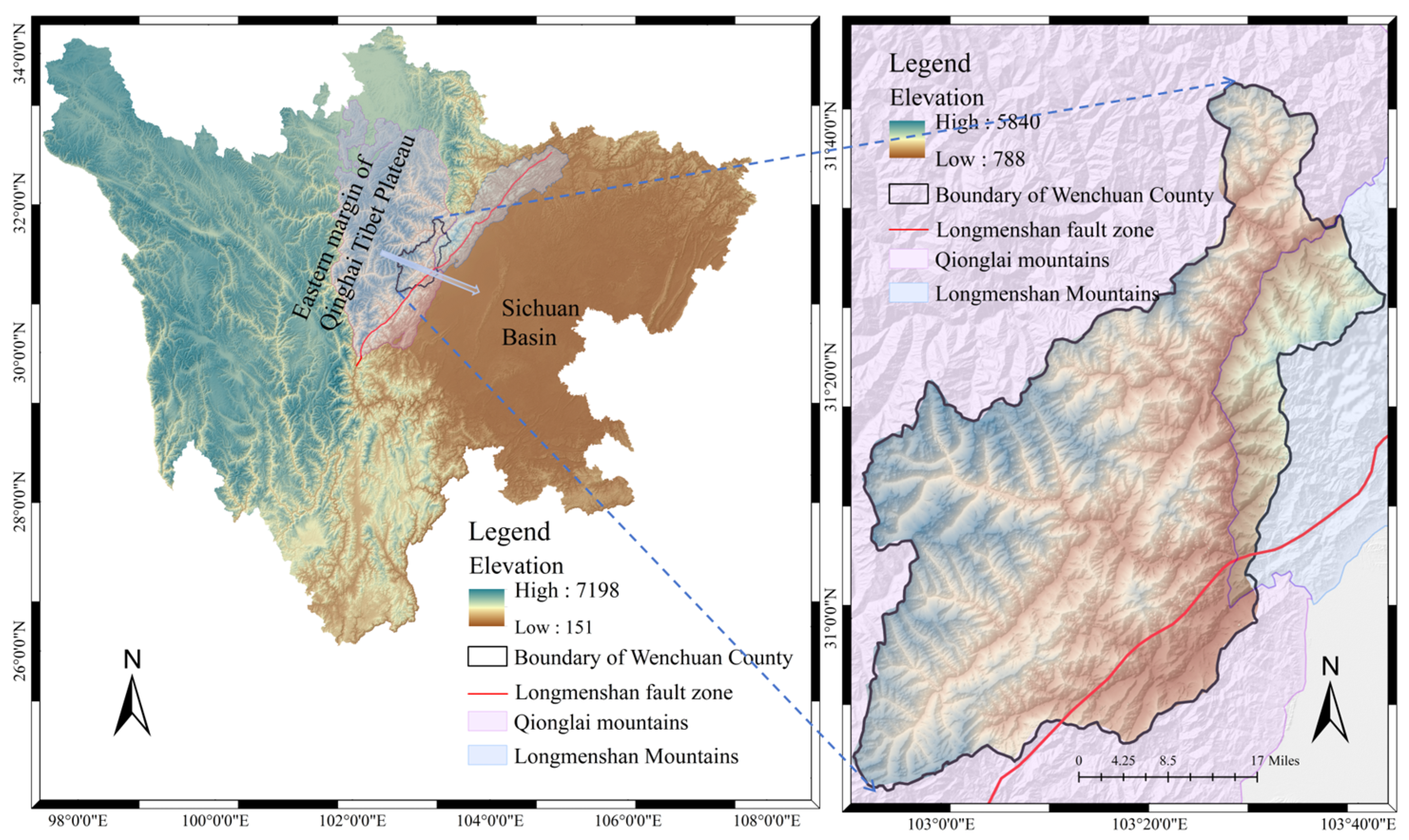
Figure 1. Geographic location and topographical features of Wenchuan County.
Water 17 02460 g001
Figure 2. The overall methodology flowchart.
Water 17 02460 g002
Figure 3. Stacking ensemble model architecture.
Water 17 02460 g003
Figure 4. ROC curves: (a) stacking ensemble model; (b) Stacking-RF model.
Water 17 02460 g004
Figure 5. Global debris-flow susceptibility mapping, based on the stacking ensemble model.
Water 17 02460 g005
Figure 6. Stacking-RF model: (a) debris-flow susceptibility mapping; (b) proportional areal distribution of the susceptibility classes.
Water 17 02460 g006
Figure 7. Location of Qingchuan County.
Water 17 02460 g007
Figure 8. Debris-flow susceptibility zonation: (a) conventional RF model; (b) Stacking-RF model.
Water 17 02460 g008
Figure 9. Global explanation: (a) factor importance ranking; (b) SHAP value summary plot.
Water 17 02460 g009
Figure 10. The driving mechanism of the sample with the highest predicted probability of debris-flow occurrence.
Water 17 02460 g010
Figure 11. Suppression mechanism of samples with the lowest predicted probability of debris-flow occurrence.
Water 17 02460 g011
Figure 12. Conditioning factor dependency: (a) distance from the road; (b) POI kernel density; (c) elevation.
Water 17 02460 g012
Figure 13. Global explanation: (a) factor importance ranking; (b) SHAP summary plot.
Water 17 02460 g013
Figure 14. Force plot: (a) The sample with the highest predicted probability; (b) The sample with the lowest predicted probability.
Water 17 02460 g014
Table 1. Comparison of the initial model validation metrics.
ModelsDatasetACCRecallF1-ScorePrecisionAUC
LRTraining set0.87660.88460.87900.87340.8765
Testing set0.81820.87500.82350.77780.8704
RFTraining set0.99351.00000.99360.98730.9934
Testing set0.80300.90620.81690.74360.8952
NBTraining set0.70130.46150.61020.90000.7045
Testing set0.72730.50000.64000.88890.8575
DTTraining set0.99350.98720.99351.00000.9936
Testing set0.80300.78120.79370.80650.8024
GBDTTraining set0.99351.00000.99360.98730.9934
Testing set0.80300.90620.81690.74360.9035
SVMTraining set0.62990.33330.47710.83870.6338
Testing set0.60610.21880.35000.87500.6769
Table 2. Performance evaluation of the stacking ensemble model and the Stacking-RF model.
ModelsDatasetACCRecallF1-ScorePrecisionAUC
Stacking ensemble modelTraining set0.98051.00000.98110.96300.9979
Testing set0.81820.87500.82350.77780.9044
Stacking-RF modelTraining set1.00001.00001.00001.00001.0000
Testing set0.96970.93750.96771.00000.9931
Table 3. Susceptibility zonation performance comparison.
ModelsRFStacking-RF
Susceptibility LevelsHistorical Disaster EventsProportion of Historical DisastersDisaster Events DensityHistorical Disaster EventsProportion of Historical DisastersDisaster Events Density
Very low1719.32%0.0194 00.00%0.0000
Low4551.14%0.0225 2022.73%0.0186
Medium2225.00%0.0348 2123.86%0.0244
High44.55%0.0626 3944.32%0.0268
Very high00.00%0.0000 89.09%0.0469
Disclaimer/Publisher’s Note: The statements, opinions and data contained in all publications are solely those of the individual author(s) and contributor(s) and not of MDPI and/or the editor(s). MDPI and/or the editor(s) disclaim responsibility for any injury to people or property resulting from any ideas, methods, instructions or products referred to in the content.