A Bayesian Ensemble Learning-Based Scheme for Real-Time Error Correction of Flood Forecasting

Abstract

To address the critical demand for high-precision forecasts in flood management, real-time error correction techniques are increasingly implemented to improve the accuracy and operational reliability of the hydrological prediction framework. However, developing a robust error correction scheme remains a significant challenge due to the compounded errors inherent in hydrological modeling frameworks. In this study, a Bayesian ensemble learning-based correction (BELC) scheme is proposed which integrates hydrological modeling with multiple machine learning methods to enhance real-time error correction for flood forecasting. The Xin’anjiang (XAJ) model is selected as the hydrological model for this study, given its proven effectiveness in flood forecasting across humid and semi-humid regions, combining structural simplicity with demonstrated predictive accuracy. The BELC scheme straightforwardly post-processes the output of the XAJ model under the Bayesian ensemble learning framework. Four machine learning methods are implemented as base learners: long short-term memory (LSTM) networks, a light gradient-boosting machine (LGBM), temporal convolutional networks (TCN), and random forest (RF). Optimal weights for all base learners are determined by the K-means clustering technique and Bayesian optimization in the BELC scheme. Four baseline schemes constructed by base learners and three ensemble learning-based schemes are also built for comparison purposes. The performance of the BELC scheme is systematically evaluated in the Hengshan Reservoir watershed (Fenghua City, China). Results indicate the following: (1) The BELC scheme achieves better performance in both accuracy and robustness compared to the four baseline schemes and three ensemble learning-based schemes. The average performance metrics for 1–3 h lead times are 0.95 (NSE), 0.92 (KGE), 24.25 ${\mathrm{m}}^3/\mathrm{s}$ (RMSE), and 8.71% (RPE), with a PTE consistently below 1 h in advance. (2) The K-means clustering technique proves particularly effective with the ensemble learning framework for high flow ranges, where the correction performance exhibits an increment of 62%, 100%, and 100% for 1 h, 2 h, and 3 h lead hours, respectively. Overall, the BELC scheme demonstrates the potential of a Bayesian ensemble learning framework in improving real-time error correction of flood forecasting systems.

1. Introduction

Hydrological models are essential rainfall–runoff simulation tools which significantly contribute to flood management and disaster mitigation [1,2]. Common hydrological models for flood management can typically be categorized into three groups: conceptual models (e.g., XAJ [3], TANK [4]), physical models (e.g., TOPMODEL [5], MIKE SHE [6]), and distributed models (e.g., VIC [7], SWAT [8]). However, due to errors induced by input data, model parameters, and numerical schemes, the performance of hydrological models often varies and fails to meet practical requirements [9,10]. Real-time error correction techniques serve as an important approach for improving the flood forecasting accuracy of hydrological models by integrating the real-time observed data with the predictions, updating the state variables, adapting key parameters, or post-processing the output. Therefore, forecasting errors can be reduced through feedback mechanisms so as to enhance the flood forecasting accuracy and robustness [11,12].

In recent years, machine learning-based techniques have been increasingly adopted in the field of real-time error correction for flood forecasting. These error correction methods can be categorized into two groups: correction for data errors (CDE) and correction for prediction errors (CPE). CDE aims to eliminate errors from the input data by pre-preprocessing, bias adjustment, and data assimilation: Zhang et al. [13] developed a CNN-LSTM hybrid deep learning framework for precipitation forecast error correction, which effectively reduced the errors of input data. Yang et al. [14] combined ridge estimation techniques with the least-squares method to construct a new error correction framework, which significantly improved error correction and forecast accuracy. Unlike data-focused CDE approaches, CPE methods are more straightforward, modifying forecast outputs through machine learning-based techniques: Guo et al. [15] systematically evaluated the numerical performance of seven machine learning methods, including Support Vector Regression (SVR), Extreme Gradient Boosting (XGBoost), the LGBM, and LSTM, in river water level forecasting, and their results showed that these models significantly reduced the forecasting errors regarding flood arrival time and effectively improved the overall performance of water level forecasting. Wang et al. [16] proposed a hybrid model which integrates observed precipitation data and the simulation results of distributed models, and their results demonstrated that the proposed deep learning approach substantially enhanced the accuracy of flood forecasting. Furthermore, the hybrid model exhibited superior performance compared to individual models, achieving more effective error correction and predictive capability.

In machine learning-based CPE methods, ensemble learning methods combine the superiorities of diverse base learners, thus minimizing individual flaws, maintaining both accuracy and robustness theoretically [17,18,19]. Despite the theoretical superiority demonstrated by ensemble learning methods, some studies revealed that the improvement of accuracy for ensemble learning models was limited, depending on how model weights were assigned [20,21]. Consequently, elucidating the underlying interaction mechanisms among base learners persists as a critical research gap in advancing ensemble learning methodologies for flood forecasting systems. A further operational challenge arises from the highly nonlinear nature of flood processes [22,23,24] in small mountainous watersheds. For instance, the floods in the Hengshan Reservoir basin exhibit significantly different dynamic characteristics across flow intervals, presenting challenges for conventional conceptual models (e.g., XAJ).

Targeting the identified knowledge gap, this study proposes a Bayesian ensemble learning-based correction scheme as a new CPE method to enhance the accuracy and reliability of the XAJ model-based flood forecasting system for the Hengshan Reservoir basin while providing data support for ensemble learning applications in flood prediction research. The numerical performance of the BELC scheme is systematically evaluated by comparison with four baseline schemes and three ensemble learning-based schemes for the Hengshan Reservoir basin. Specifically, the main objectives of this study are as follows:

i.  

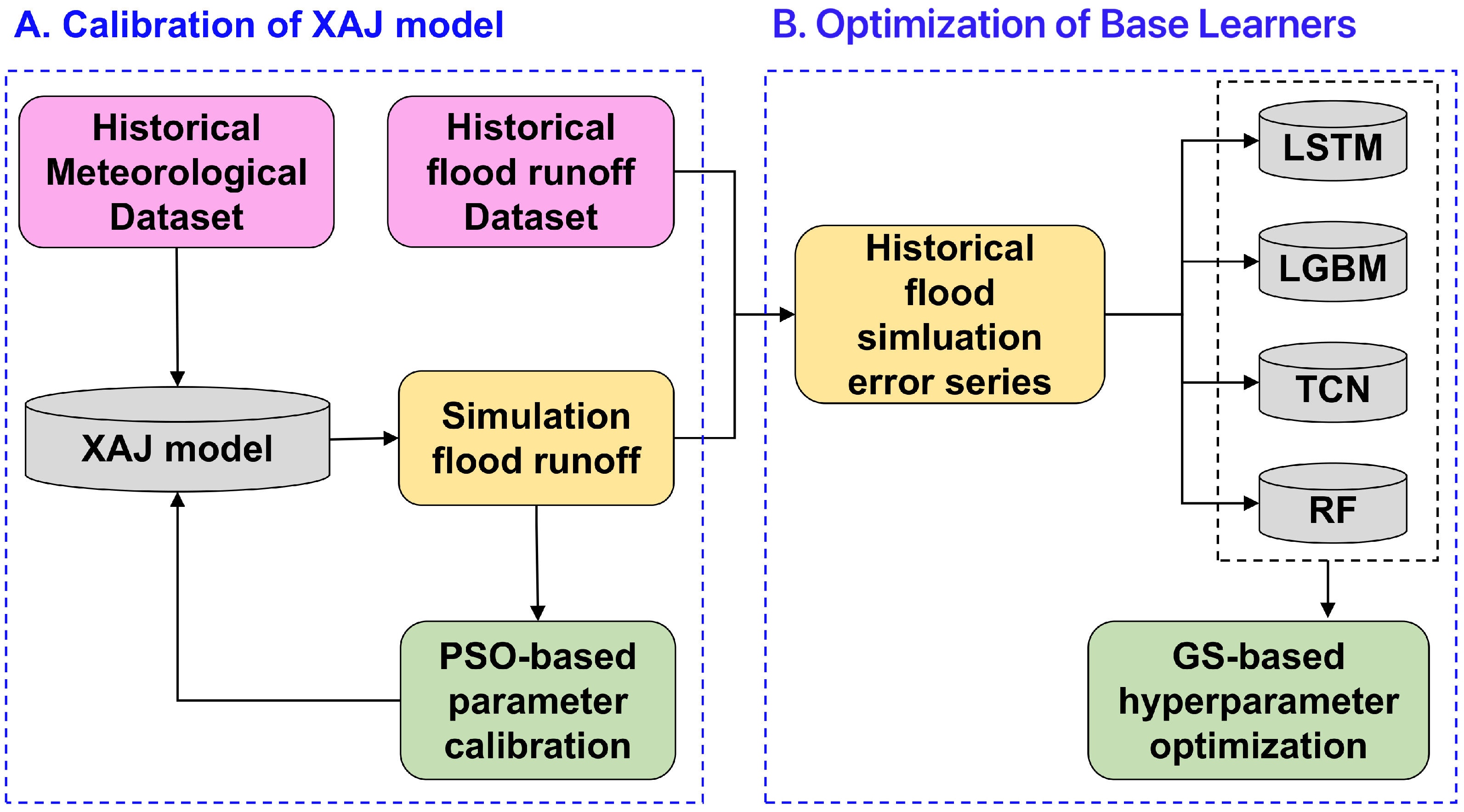
To develop a new error correction scheme based on the Bayesian ensemble learning framework by integrating the XAJ model and four base learners, and to evaluate its suitability for application in the Hengshan Reservoir basin;

ii. 

To evaluate the characteristics of the proposed scheme by comparing it with baseline schemes, and to provide data support for research on ensemble learning frameworks in flood forecasting;

iii.

To investigate the potential of the K-means clustering technique under the Bayesian ensemble learning framework.

2. Materials and Methods

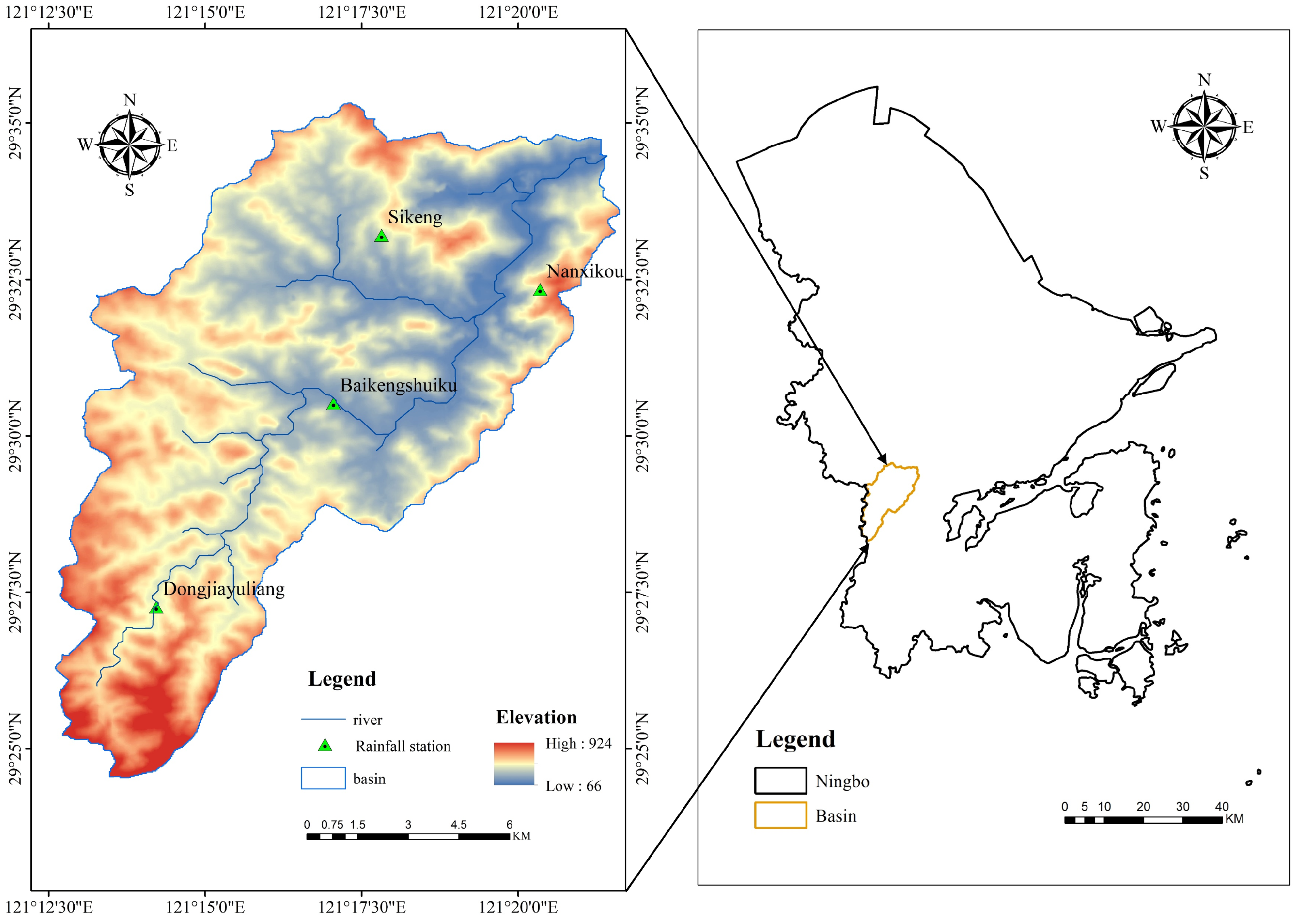
2.1. Study Area and Data Sources

The study area Hengshan Reservoir basin(Fenghua Hydrological Bureau and Hengshan Reservoir Management Station, Ningbo, China) lies in the headwaters of the Xin’anjiang River system and controls a drainage area of 181 ${\mathrm{km}}^2$. The general situation of the catchment and the spatial distribution of the rain gauge stations are shown in Figure 1. The reservoir lies within a subtropical monsoon climate zone characterized by an average annual temperature of about 16.3 °C and an annual rainfall of 1350–1600 mm. Affected by the climate, the basin floods show typical rainstorm flood characteristics. The annual maximum floods mostly occur in the Meiyu period from June to August, and the continuous rainstorm process in this stage is prone to causing high-intensity runoff generation and concentration. In terms of topographical features, the Hengshan Reservoir basin is characterized by significant terrain undulations, dominated by hills and low mountains. The lowest point in the north-eastern part lies at 66 m, while the highest point in the south-western part reaches 924 m. After heavy rainfall, rainwater in the surrounding mountainous areas converges rapidly, resulting in short durations of runoff generation and confluence. Hengshan Reservoir, as a large-scale and important water conservancy project in the upper reaches of the Xin’anjiang River, plays a crucial role in flood storage and regulation, mitigating flood disasters in downstream areas, and ecological protection. Due to the small drainage area above Hengshan Reservoir, runoff generation occurs rapidly, resulting in high-magnitude peak discharges. In practice, the conventional XAJ model struggles to accurately estimate the arrival time and magnitude of the flood peak, significantly impacting reservoir operation decisions and evacuation timelines. Against this background, the construction of a high-precision flood forecasting model is of great significance for reducing the casualties and property losses caused by floods. In particular, under the condition of scarce input data, improving the forecasting accuracy while extending the forecast horizon has become a core engineering problem that urgently needs to be solved in the flood forecasting of the Hengshan Reservoir basin. The research results can also provide a scientific basis for flood control decision-making and water resource allocation.

The Fenghua Hydrological Bureau and the Hengshan Reservoir Management Station have provided hydrological data for 14 flood events from 1997 to 2024. These 14 flood events cover different magnitudes and types (single-peak and double-peak), ensuring that the selection of flood events is broadly representative. The data includes the inflow discharge of Hengshan Reservoir, the average areal evapotranspiration of the basin, and the rainfall amounts of 4 rainfall stations with a time interval of 1 h. The digital elevation data is the SRTM DEM product (resolution of 30 m). The 14 flood events are divided into calibration and validation periods at a ratio of 4:3 for calibration of the hydrological model and the machine learning technique. The validation period is further divided into two subsets at a 1:1 ratio for comparison of the integrated error correction.

2.2. Hydrological Model

The Xin’anjiang (XAJ) model was first proposed by Zhao Renjun [25] in 1963. With low requirements for input data, this model has been widely applied to flood forecasting in the humid and semi-humid regions of China and has achieved high forecasting accuracy. Due to the small watershed area of the study region, the scarcity of hydrological stations, and the lack of long-term measured flood data, this model was selected for flood simulation and forecasting in the study area. It is mainly composed of four parts: evapotranspiration calculation, runoff generation calculation, water source separation calculation, and flow concentration calculation. The XAJ model uses sub-basins as basic hydrological units, and the outflow calculation process for each sub-basin is as follows: Firstly, a three-layer structure (upper layer, lower layer, deep layer) is adopted to calculate evapotranspiration. Secondly, runoff generation is determined based on rainfall and soil water deficit, and the tension water capacity distribution curve is used to reflect the non-uniform distribution characteristics of the tension water capacity within the sub-basin. Thirdly, according to the free water capacity distribution curve, total runoff is subdivided into surface runoff, interflow, and groundwater runoff. Fourthly, surface runoff, interflow, and groundwater runoff are concentrated to the outlet of each sub-basin through linear reservoirs. Finally, the outflow of each sub-basin is connected through the river network, and the Muskingum flow concentration model is used to route it to the outlet of the entire basin.

2.3. Machine Learning Methods

Real-time flood correction requires processing hydrological data with strong temporal dependence and complex nonlinearity. According to previous research experience in the field of hydrology and the practical application performance of models in flood forecasting [15,26,27], LSTM and TCN can capture temporal dependence through gating mechanisms and dilated causal convolutions. The LightGBM and RF can efficiently handle high-dimensional data and fit nonlinear mappings. Therefore, this study selected LSTM, the LGBM, TCN, and RF as the base learners for real-time correction of flood discharge errors.

2.3.1. Long Short-Term Memory (LSTM) Networks

LSTM was first proposed by Hochreiter et al. [28] to address the shortcomings of Recurrent Neural Networks (RNNs) in handling long time series, such as gradient vanishing, gradient explosion, and difficulty in capturing long-term dependencies. LSTM stores long-term information in sequences by introducing a unique memory cell while designing input gates, forget gates, and output gates to precisely regulate information flow. Therefore, LSTM can not only effectively capture the temporal dependencies in time series data but also solve the problem of long-term dependencies. Due to its characteristics matching the needs of flow forecasting in the hydrological field, LSTM has become a widely used deep learning model in hydrological flow forecasting [29,30].

2.3.2. Light Gradient-Boosting Machine (LGBM)

Proposed by Ke et al. [31] in late 2016, the LGBM achieves its implementation principle by utilizing the CART to iteratively train data to obtain an optimal model. The specific procedure involves sequentially training a series of CARTs, generating a weak classifier in each iteration, where the weak classifier in the next round continues to train on the residuals of the previous weak classifier. Finally, the prediction results of all regression trees collectively constitute the model output. Different from traditional methods, the LightGBM employs a histogram algorithm to discretize data to optimize the optimal CART splitting points and adopts a leaf-wise growth strategy. Unlike traditional level-wise growth, this strategy can more rapidly reduce the loss function value, thereby enhancing network performance and scalability. Therefore, the LightGBM features high efficiency, high precision, strong scalability, and the advantage of being less prone to overfitting. It is suitable for various machine learning tasks and has been widely applied in hydrological flow forecasting research [32,33].

2.3.3. Temporal Convolutional Networks (TCNs)

A TCN is a novel deep learning model tailored for time series analysis which incorporates causal convolution, dilated convolution, and residual connections into its architecture [34]. Distinct from RNNs and LSTM, a TCN leverages convolution operations to capture sequential dependencies, enabling parallel processing of multiple data points. This not only enhances its capability to handle large datasets efficiently but also reduces training time. By stacking convolutional layers for feature extraction, utilizing residual connections to optimize learning, and employing dilated convolutions to expand the receptive field, the TCN effectively mitigates gradient vanishing or explosion issues and manages long-term dependencies. Characterized by high computational efficiency and long-term memory retention, the TCN has emerged as a prevalent deep learning model in hydrological flow forecasting research [26,34].

2.3.4. Random Forest (RF)

RF was proposed by Breiman [35] based on the Bagging ensemble learning theory. Its core concept involves constructing a forest model composed of numerous decision trees where each tree grows independently using a random subset of the training dataset and a random subset of features. The final prediction is achieved through a voting mechanism (for classification tasks) or averaging (for regression tasks), resulting in a single consensus prediction. This “collective decision-making” approach effectively mitigates the overfitting risk inherent in individual decision trees and significantly enhances the model’s generalization capability. Owing to its strong nonlinear fitting ability, high tolerance to data noise, and efficient parallel computing characteristics, RF has demonstrated feasibility in time series forecasting and hydrological flow prediction [27,36].

2.4. Bayesian Ensemble Learning-Based Correction Scheme

2.4.1. Preprocessing

As illustrated in Figure 2, the XAJ model was first calibrated by the particle swarm optimization (PSO) algorithm. A total of 10 sensitive parameters were selected for calibration, involving evapotranspiration, runoff generation, water source separation, and flow concentration processes. The results of the calibrated parameters are presented in

Table 1. Parameters of the XAJ model.

Parameters	Description	Value
KC	Ratio of potential evapotranspiration to pan evaporation	0.667
WUM	Tension water capacity of upper layer, mm	32.84
WLM	Tension water capacity of lower layer, mm	89
SM	Free water storage capacity, mm	9.71
KG	Outflow coefficient of free water storage to groundwater flow	0.01
KI	Outflow coefficient of free water storage to interflow	0.7
CS	Recession coefficient of surface runoff	0.632
CI	Recession coefficient of interflow	0.769
CG	Recession coefficient of groundwater	0.999
XE	Muskingum weighting factor	0.1

. Then, the historical flood simulation error series was constructed by the XAJ simulation results and the historical flood runoff dataset during the calibration period. Finally, the mapping relationship of input–target pairs of the error sequence was fitted for every machine learning technique using the grid search (GS) method, and the optimal hyperparameter combinations for the four machine learning methods are listed in

Table 2. Summary of optimal parameters for different machine learning methods.

Models	Description and Value Range	Value
	Number of estimators: 100–1000	200
LGBM	Learning rate: 0.001–0.3	0.1
	Max. depth: 3–20	3
	Number of epochs: 10–200	50
LSTM	Learning rate: 0.0001–0.1	0.01
	Batch size: 8–128	16
	Number of epochs: 10–200	50
TCN	Learning rate: 0.0001–0.1	0.01
	Batch size: 32–512	128
	Number of estimators: 100–1000	200
RF	Max. depth: 3–50	10
	Minimum samples per node: 2–20	5

.

The BELC scheme primarily consists of three key components: generation of the basic error correction dataset (BECD), classification of the BECD based on flow ranges clustering, and optimization of the weighted combination under a Bayesian framework, as illustrated in Figure 3. The model initially processes residual data from the XAJ model’s forecast results using each base learner to obtain preliminary corrected flood forecasting outputs, which is referred to as the basic error correction dataset (BECD). Subsequently, the K-means clustering technique is employed to partition flow discharge data into distinct ranges. Finally, the Bayesian ensemble model is trained based on the BECD using the flow interval clustering results. Using the Nash–Sutcliffe efficiency (NSE) as the objective function, the model optimizes the base learner weights for different discharge intervals. Upon reaching the preset iteration count, it weights the BECD results according to the optimal contribution combination to produce the final integrated flood discharge outputs.

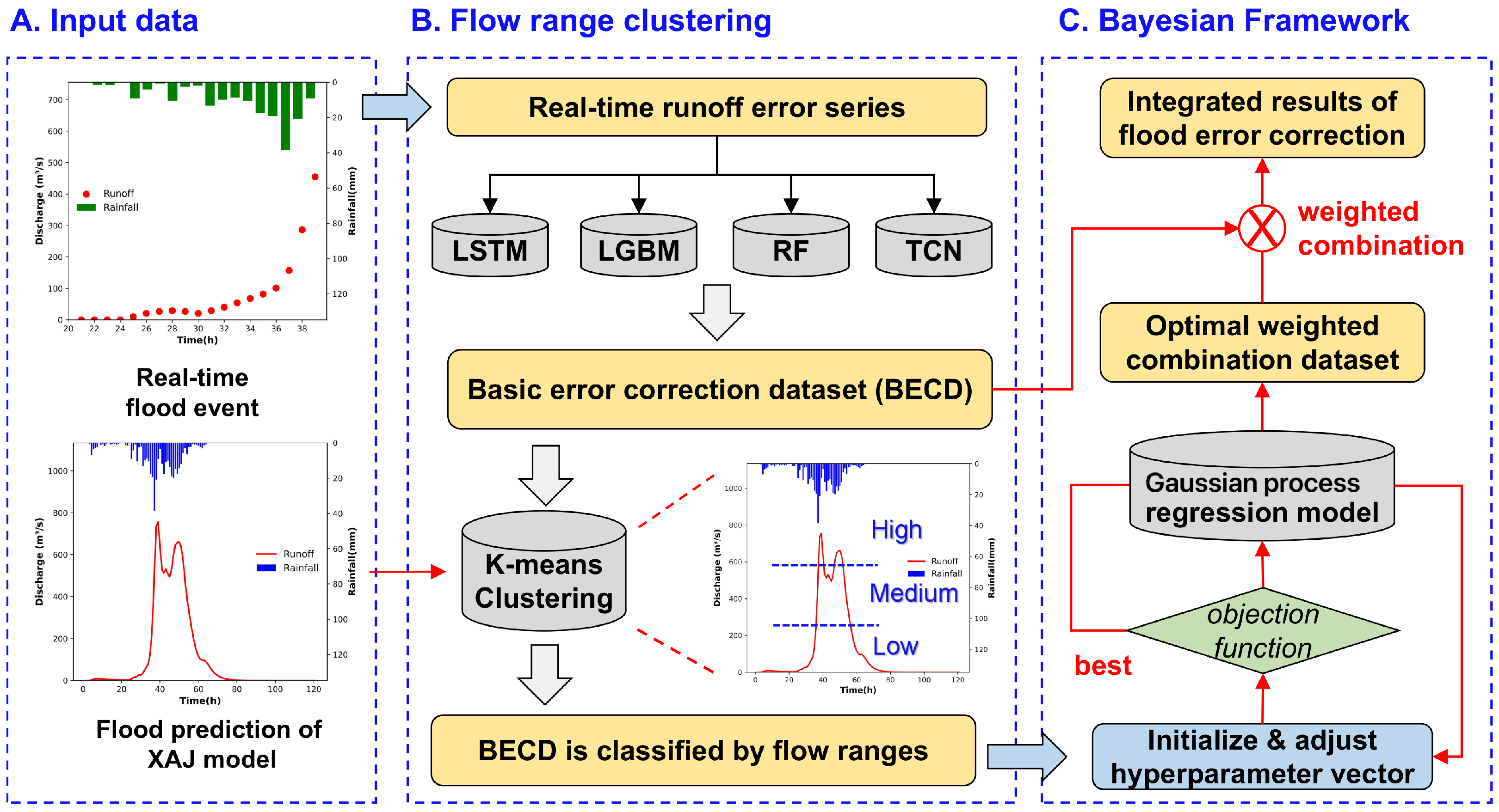
2.4.2. Generation of Basic Error Correction Dataset (BECD)

Based on the flood forecasting results from the XAJ model and the real-time flood event, Equation (1) was used to calculate the difference between the observed and forecasted flow, thereby constructing a real-time runoff error series. Following the AIC, for each time step, the current residual and two prior residuals were employed to form valid input–target pairs, generating error series samples for lead times of 1, 2, and 3 h. Subsequently, each base learner was applied to fit the mapping relationships between the input–target pairs of these error series samples for each lead time. Finally, the BECD was constructed using Equation (2).

$$\Delta Q\left(t\right)=Q_{obv}\left(t\right)-Q_{sim}\left(t\right)$$

(1)

$${\{\Delta Q(t+i)\}}_{i=1,2,3}=f(\Delta Q\left(t\right),\Delta Q(t-1))$$

(2)

where $\Delta Q\left(t\right)$ represents the runoff error between observed value $Q_{obv}\left(t\right)$ and hydrological simulation value $Q_{sim}\left(t\right)$ at time t, $\{\Delta Q(t+i\left)\right\}$ denotes the collection of runoff prediction errors across i forward time steps, obtained by the regression function of each base learner, and i represents the lead time duration.

2.4.3. Classification of BECD Based on Flow Range Clustering

The K-means clustering technique partitions data into K distinct clusters by maximizing intra-group similarity and inter-group differences. In this study, the selection of the K value was primarily determined based on the empirical findings of previous research [37,38,39,40]. The classification of flood discharge into three physically distinct ranges (high, medium, low) also reflects hydrological response characteristics. The main processes were as follows:

i. 

Randomly selecting three initial cluster centers $C_i(1\le i\le 3)$ from the simulation flood flow discharge dataset, calculating the Euclidean distance (Equation (3)) between the remaining data objects and the cluster center $C_i$, finding the cluster center $C_i$ closest to the target data object, and assigning the data object to the cluster corresponding to the cluster center $C_i$.

ii.

Updating cluster centers by calculating the average value of the data objects in each cluster. The iteration process terminates when either the Sum of Squared Errors(SSE) (Equation (4)) of all clusters converges or the predefined maximum number of iterations is reached.

$$d(x,C_i)=\sqrt{{\displaystyle \sum _{j=1}^m}{(x_j-C_{ij})}^2}$$

(3)

$$\mathrm{SSE}=\sum _{i=1}^k\sum _{x\in C_i}{\left|d(x_j,C_{ij})\right|}^2$$

(4)

where x represents the data object, $C_i$ represents the i-th cluster center, m represents the dimension of the data object, and $x_j$ and $C_{ij}$ represent the j-th attribute values of x and $C_i$, respectively.

2.4.4. Optimization Under Bayesian Ensemble Learning Framework

The Bayesian algorithm is a global optimization algorithm for serial models which can handle multiple variables simultaneously, solve the relationships among variables in optimization problems, adaptively adjust the positions of sampling points with a small number of samples, and quickly search for the optimal parameter configuration within a given parameter space [41,42]. The core of Bayesian optimization lies in using models such as Gaussian process regression to estimate the distribution of the objective function and selecting the optimal parameter combination based on this distribution. A new evaluation point is selected each time, and its potential is evaluated through an acquisition function, so as to efficiently approach the global optimal solution within a limited number of evaluations [43]. The probabilistic model employed in this study is Gaussian process regression (GPR), with the acquisition function set to expected improvement (EI). The basic process for constructing the Bayesian ensemble learning framework is listed below:

Step 1: Initialize hyperparameter vectors: Set weight parameters for each base learner according to each flow interval. The initial weight is set to 0.25 for each base learner. The weights for each flow interval are normalized to ensure their summation equals unity.

Step 2: Generate initial evaluation datasets: For each flood event, calculate the weighted flood flow correction values within each flow interval based on the initialized weights of the base learners, as shown in Equation (5):

$$\tilde{\mathbf{Q}}=\sum _i^n{\mathbf{w}}_i·{\mathbf{Q}}_i$$

(5)

where $\tilde{\mathbf{Q}}$, ${\mathbf{w}}_i$, and ${\mathbf{Q}}_i$ represent the set of weighted correction values, weights calculated by the i-th base learner, and the flow value in the classified BECD for each flow interval.

Step 3: Objective function calculation: Compute the Bayesian objective function value based on the weighted flow correction values from each flood event. The objective function is defined as the maximization of the Nash—Sutcliffe efficiency coefficient (NSE), as expressed in Equation (6):

$$\mathrm{NSE}=1-{\displaystyle \frac{{\displaystyle \sum _{i=1}^N}[Q_{obs}\left(i\right)-{\tilde{Q}}_{sim}\left(i\right)]}{{\displaystyle \sum _{i=1}^N}{[Q_{obs}\left(i\right)-{\overline{Q}}_{obs}]}^2}}$$

(6)

where $Q_{obs}$, ${\overline{Q}}_{obs}$, $Q_{sim}$, and ${\tilde{Q}}_{sim}$ represent the observed flow, the mean value of the observed flow, the simulation flow by the XAJ model, and the simulation flow after real-time error correction, respectively;

Step 4: Next evaluation point selection: Employ a Gaussian process regression model (Equation (7)) to maximize the acquisition function, thereby identifying the parameter combination that minimizes the objective function value:

$$x_t=\mathbf{argMax}\left[a\left(x\right|D_{t-1})\right]$$

(7)

where $x_t$ represents the next parameter combination selected in the t-th iteration, and $D_{t-1}$ represents the historical evaluation data up to the prior iteration, including all previous parameter combinations and their corresponding objective values. $a\left(x\right|D_{t-1})$ represents the acquisition function that determines which weight combination to choose for maximizing objective improvement based on the current evaluation dataset.

Step 5: Update the evaluation dataset by incorporating the newly evaluated point and its corresponding results using Equation (8), thereby progressively refining the dataset:

$$D_t=D_{t-1}\cup \left\{[x_t,f\left(x_t\right)]\right\}$$

(8)

where $D_t$ represents the evaluation dataset at the t-th iteration, $D_{t-1}$ represents the updated evaluation dataset at the prior iteration, $x_i$ represents the currently selected parameter combination, and $f\left(x_i\right)$ represents the current objective function value.

Step 6: Stopping criteria and result output: Set a maximum number of iterations. When the number of iterations reaches the maximum, stop the algorithm iteration and obtain the optimal parameter combination (weight combinations of each base learner in different flow intervals) from the evaluation point set, which is the parameter combination that minimizes the objective function value.

2.4.5. Evaluation Metrics of Flood Correction

In addition to the NSE introduced before, four additional metrics, the Kling–Gupta Efficiency Coefficient (KGE), the Root Mean Square Error (RMSE), the relative error of runoff depth (RPE), and the absolute error of peak time (PTE), were selected to quantitatively assess the numerical performance of the real-time error correction scheme, and are evaluated as follows:

$$\mathrm{KGE}=1-\sqrt{{(r-1)}^2+{(\beta -1)}^2+{(\gamma -1)}^2}$$

(9)

$$\mathrm{RMSE}=\sqrt{{\displaystyle \frac{1}{N}}\sum _{i=1}^N{[Q_{obs}\left(i\right)-{\tilde{Q}}_{sim}\left(i\right)]}^2}$$

(10)

$$\mathrm{RPE}={\displaystyle \frac{Q_{peak,sim}-Q_{peak,obs}}{Q_{peak,obs}}}\times 100\%$$

(11)

$$\mathrm{PTE}=T_{peak,obs}-T_{peak,sim}$$

(12)

In Equation (9), r, $\beta$, and $\gamma$ are the Pearson correlation coefficient, the bias ratio, and the variability ratio between observed and simulated values. The KGE equally weights correlation, bias, and variability, which is less sensitive to extreme outliers compared to the NSE [44]. In Equation (10), N represents the number of observations. In Equations (11) and (12), $Q_{peak,obs}$ and $Q_{peak,sim}$ donate the observed and the simulated peak flow, respectively. $T_{peak,obs}$ and $T_{peak,sim}$ represent the corresponding arrival times for the observed and simulated peak flow.

This study adhered to China’s national standard GB/T 22482-2008 [45] (Technical Guidelines for Hydrological Forecasting), which defines the following qualification criteria for flood forecasts:

i.  

NSE > 0.7;

ii. 

RMSE < 15% of observed peak discharge ($Q_{peak,obs}$);

iii.

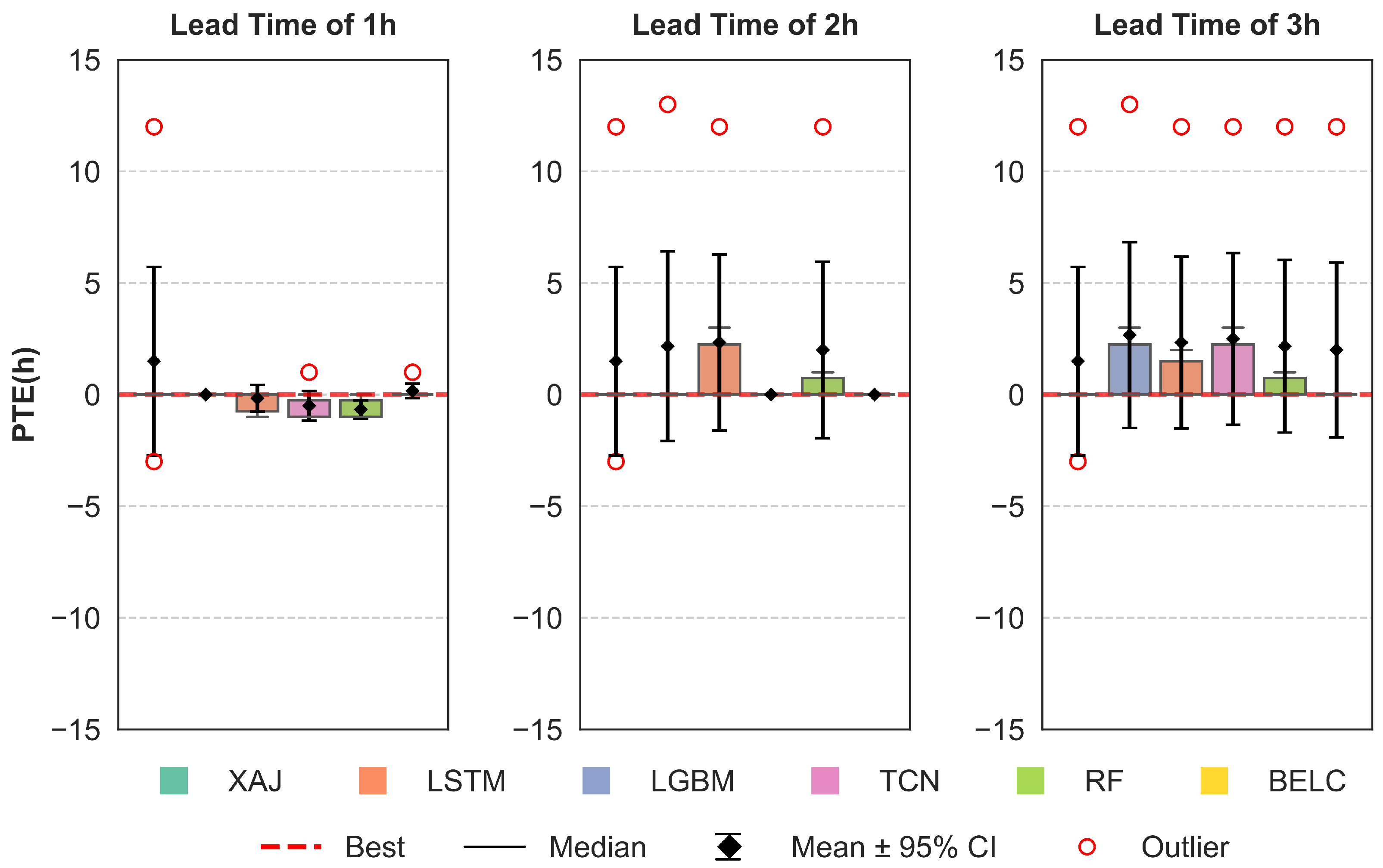
PTE must be positive and within 3 h;

iv.

RPE < 20%.

While the Kling–Gupta Efficiency (KGE) is not formally specified in the standard, a KGE value exceeding 0.75 can be considered an acceptable threshold for hydrological model performance [46].

3. Results and Discussion

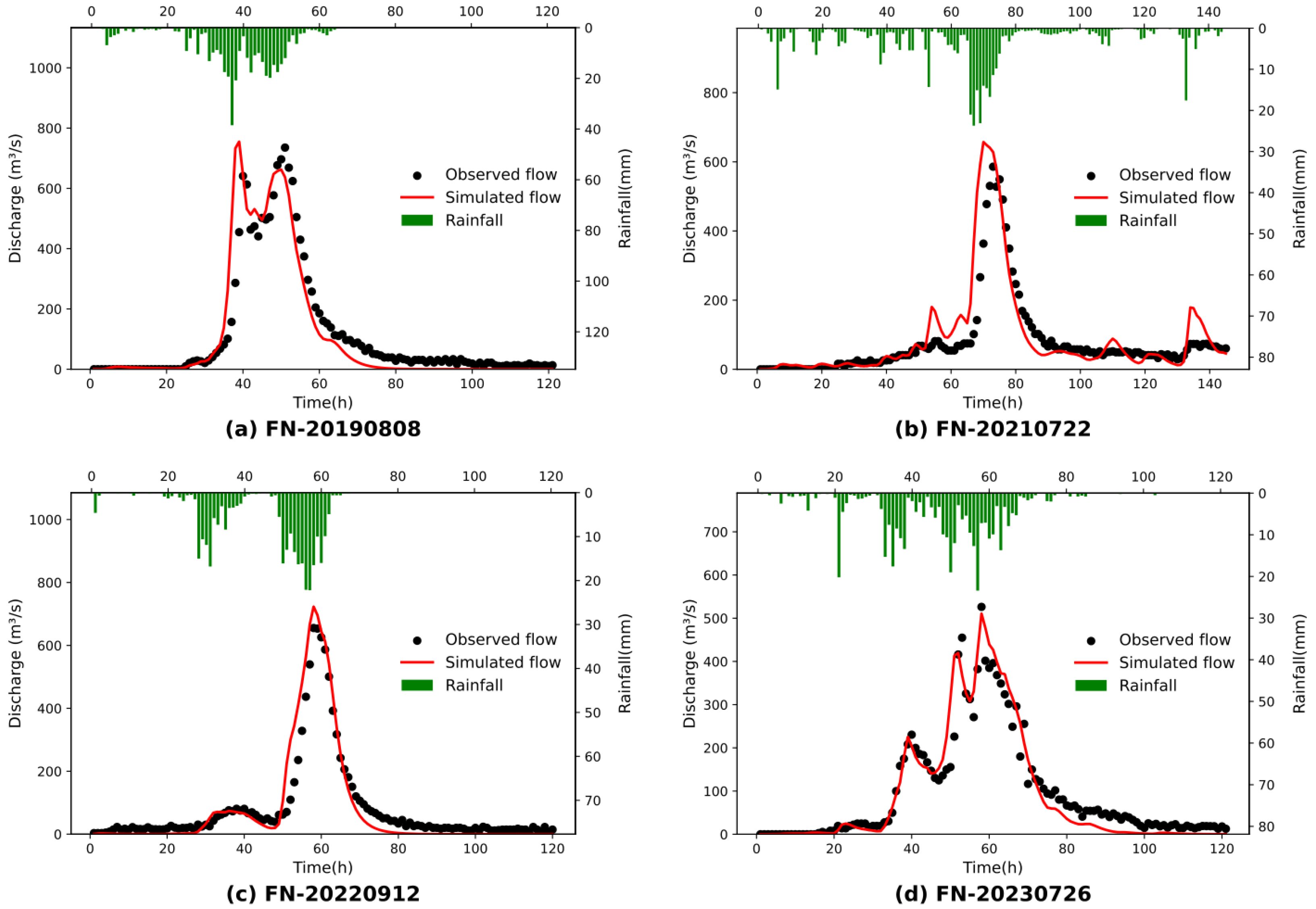
3.1. Results of the Calibrated and Validated Simulations

The XAJ model demonstrated generally reliable performance in simulating floods in the Hengshan Reservoir basin, achieving consistent Nash–Sutcliffe efficiency (NSE) values of 0.85 for both the calibration (eight floods) and validation (six floods) periods. While the XAJ model showed good temporal accuracy with peak timing errors (PTE) of under 3 h for most events, its performance in peak flow estimation was less consistent, with 37.5% of calibrated floods and 33.3% of validated floods exceeding the 20% relative peak error (RPE) threshold. The RMSE was an average of 84.68 ${\mathrm{m}}^3$/s during calibration and decreased by 44% to 47.37 ${\mathrm{m}}^3$/s in validation, implying that more stable error distribution patterns emerged during validation.The overall qualification rates were 62.5% for calibration and 50% for validation, indicating satisfactory but imperfect performance, particularly for extreme flow events.

Figure 4 shows the flood hydrographs of the XAJ simulation for four typical flood events in the validation period. The plots demonstrate that the XAJ model effectively captured the timing, peak magnitude, and recession characteristics overall. However, the numerical performance declined significantly when the flood flow fluctuated violently, resulting in only a 50% flood qualification rate during validation. For flood events (a) 20190808 and (b) 20210722, the TPE forecasting errors showed a 3-h advance and 12-h delay, respectively, both being particularly significant deviations. Consequently, it is essential to implement real-time error correction to improve the accuracy of flood forecasting results (see

Table 3. Performance metrics of the XAJ model for all flood events.

	Flood Events	RPE (%)	PTE (h)	NSE	RMSE (${\mathrm{m}}^2$/s)
Calibration	19970818	24.35	1	0.70	169.60
	20050910	18.19	0	0.96	68.06
	20071005	11.83	0	0.97	34.95
	20090006	22.40	0	0.92	70.70
	20120807	−9.99	−2	0.86	83.35
	20150710	−9.63	0	0.80	75.97
	20150928	−8.59	−1	0.77	84.46
	20160914	−2.09	−1	0.84	90.36
Validation	20200008	82.3	12	0.86	116.04
	20200102	122.3	8	0.88	65.47
	20210912	22.15	0	0.85	48.91
	20220912	103.2	8	0.89	45.56
	20230726	139.4	8	0.91	55.50
	20240724	25.74	0	0.91	17.28

).

3.2. Correction Performance Comparisons of Different Schemes

The boxplots in Figure 5, Figure 6, Figure 7, Figure 8 and Figure 9 statistically compare five key metrics (the NSE, KGE, RMSE, RPE, and PTE) for the XAJ model over all five real-time error correction schemes (LSTM, the LGBM, TCN, RF, and BELC) across three forecasting horizons (1, 2, and 3 h). As demonstrated across all boxplots, all the real correction schemes significantly improved the NSE and KGE of flood forecasting and reduced the RMSE, RPE, and PTE of the flood forecasting for all lead times. Specifically, compared with the XAJ model under a 1 h lead time, the mean NSE values of the RF, LGBM, LSTM, TCN, and BELC schemes reached 0.958, 0.952, 0.960, 0.957, and 0.964, respectively, representing increments of 5.2%, 4.6%, 5.4%, 5.1%, and 5.8%. The mean RMSE values were 20.66 ${\mathrm{m}}^3$/s, 22.77 ${\mathrm{m}}^3$/s, 19.93 ${\mathrm{m}}^3$/s, 20.59 ${\mathrm{m}}^3$/s, and 19.14 ${\mathrm{m}}^3$/s, respectively, representing reductions of 36.90%, 30.45%, 39.13%, 37.11%, and 41.53%. The mean RPE values were 8.66%, 12.14%, 8.77%, 7.85%, and 8.25%, respectively, with a reduction of 4.37%, 0.39%, 4.26%, 5.18%, and 4.78% relative to the XAJ. The mean KGE values were 0.949, 0.919, 0.951, 0.952, and 0.955, respectively, representing increments of 16.8%, 13.8%, 17.0%, 17.1%, and 17.4%. For the cases with lead times of 2 h and 3 h, the overall correction performance of all models remained consistent. Although the evaluation metrics exhibited some degradation as the lead time increased, the models still effectively improved the overall flood forecasting performance.

Figure 10 displays the simulated curves for real-time flood forecasting correction using the BELC scheme and four baseline schemes (taking flood event 20220912 with the lead time of 1 h as an example). It can be concluded from the illustration that all four baseline schemes performed well in correcting the XAJ forecasting results, while their effectiveness in local flow correction exhibited marginal variations. For instance, LSTM tended to exhibit oscillations during periods of rapid flow variation and LGBM lacked precision in capturing peak flows, while TCN and RF showed slightly larger forecasting errors in low-flow intervals. Overall, the BELC model effectively integrated the results from various base learners, maintaining both high correction accuracy and strong robustness.

Figure 11 shows a comparative scatter plot of correction errors for the BELC and four baseline schemes, where the x and y axes represent the absolute correction errors ($|\Delta Q|$) for one specific scheme. Taking “High: 5 (62%)” in Figure 11a as an example, this indicates that BELC achieved superior correction accuracy over LSTM in five high-flow instances, representing 62% of the evaluated cases.The results demonstrated that the BELC-corrected discharge $Q_{corrected}$ exhibited significantly smaller deviations from observed discharge $Q_{obs}$ compared to all four baseline schemes, especially in the high-flow interval with a smaller lead hour. While the enhancement was more modest during medium–low flow periods relative to high-flow events, the BELC scheme consistently outperformed standalone baseline schemes, providing more accurate corrections across the majority of test cases.

3.3. Comparative Performance of Ensemble Learning Frameworks

To further investigate the effect of different ensemble learning frameworks on real-time error correction, three schemes based on ensemble learning models including linear regression (LS), Support Vector Regression (SVR), and the Naive Bayes scheme without the K-means clustering technique were built for comparison.

As can be seen from

Table 4. The computational efficiency of different ensemble learning models under optimal parameter configurations.

Models	Optimal Parameters	Training Time (s)	Prediction Time (s)
Linear Stacking	Linear model: Lasso	0.06	0.0075
	Maximum iterations: 5000
	Regularization coefficient: 1
	Fit interception: True
SVR Stacking	Linear model: Lasso	1.42	0.0021
	Maximum iterations: 5000
	Regularization coefficient: 1
Naive Bayesian	Optimization iterations: 7	0.01	${10}^{-6}$
	Acquisition function: EI
	Exploration parameter: 0.01
	Number of initial DOE points: 10
BELC	Optimization iterations: 7	0.02	${10}^{-6}$
	Acquisition function: EI
	Exploration parameter: 0.01
	Number of initial DOE points: 10

Note: All experiments were implemented in Python 3.12. The hardware platform was equipped with an NVIDIA RTX 4060 GPU (NVIDIA Corporation, Santa Clara, CA, USA) with 8 GB GDDR6 memory and an Intel i9-13900HX processor (Intel Corporation, Santa Clara, CA, USA).

, single training and prediction times for each model under the optimal parameter configuration are listed. Regarding the determination of optimal parameters, convergence was assumed to be achieved when the Bayesian optimization algorithm’s objective function fluctuation amplitude was less than $1\times {10}^{-5}$ for five consecutive iterations. The optimal number of iterations was determined to be seven, and the grid search method was employed to determine the remaining parameters.

In the training phase, the Bayesian optimization algorithm can quickly converge to the optimal weights with a relatively small number of iterations. Therefore, the single training time of the Naive Bayesian and BELC schemes was only 0.01 s and 0.02 s, respectively, which is much lower than that of traditional stacked ensemble learning. In the prediction phase, the Naive Bayesian and BELC schemes achieved a microsecond-level response (${10}^{-6}$ s) through the linear weighting of base learners, significantly outperforming traditional stacked ensemble learning methods.

Therefore, the BELC scheme proposed in this paper exhibited superior computational efficiency compared to the other three schemes. Combined with its advantages in the real-time correction of flood errors, the BELC scheme demonstrated strong applicability in engineering practice.

As shown in the scatter plot of Figure 12, the comparison between the BELC scheme and the LS and SVR stacking proves that the BELC has obvious correction advantages in medium and high flow ranges, especially in the high-flow interval. Although conventional ensemble learning models had a leading correction effect in the low-flow interval, the comparison between the BELC scheme and the Naive Bayesian scheme indicated that the K-means clustering technique can greatly improve the real-time error correction performance in the high-flow interval for all lead time scenarios (e.g., 62%, 100%, and 100%), which is of vital importance in flood forecasting.

4. Conclusions

This study proposed the Bayesian ensemble learning correction (BELC) scheme, a novel framework for real-time flood forecast error correction. Four base learners (Random Forest, the LightGBM, LSTM, and TCN) were integrated with the K-means clustering technique to post-process XAJ model outputs. By comparing the numerical performance of the BELC scheme with four baseline schemes constructed by base learners and three ensemble learning schemes, the BELC scheme demonstrated the potential of the Bayesian ensemble learning framework and the K-means flow range clustering technique in improving flood forecasting systems. The main conclusions are summarized as follows:

i.  

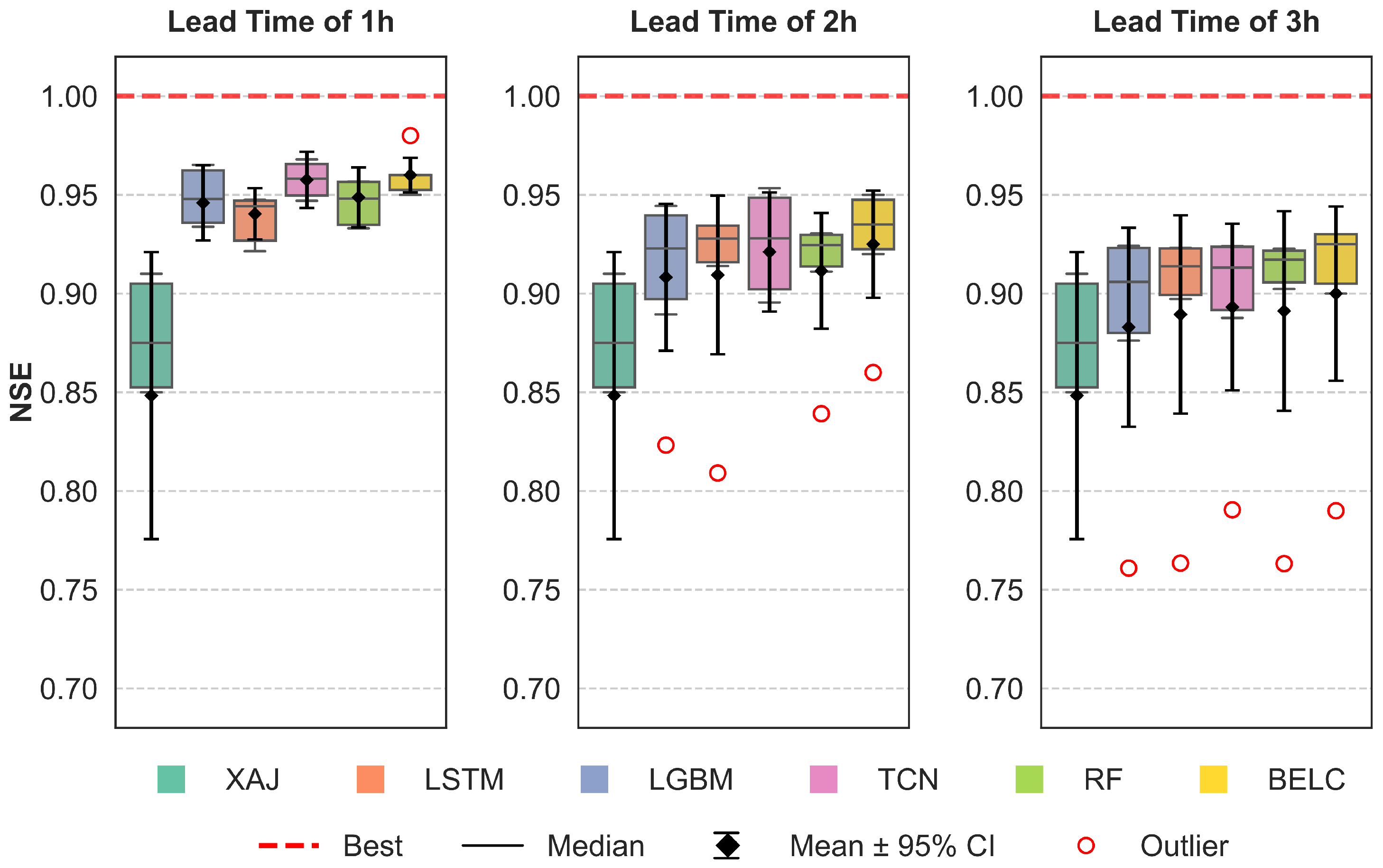
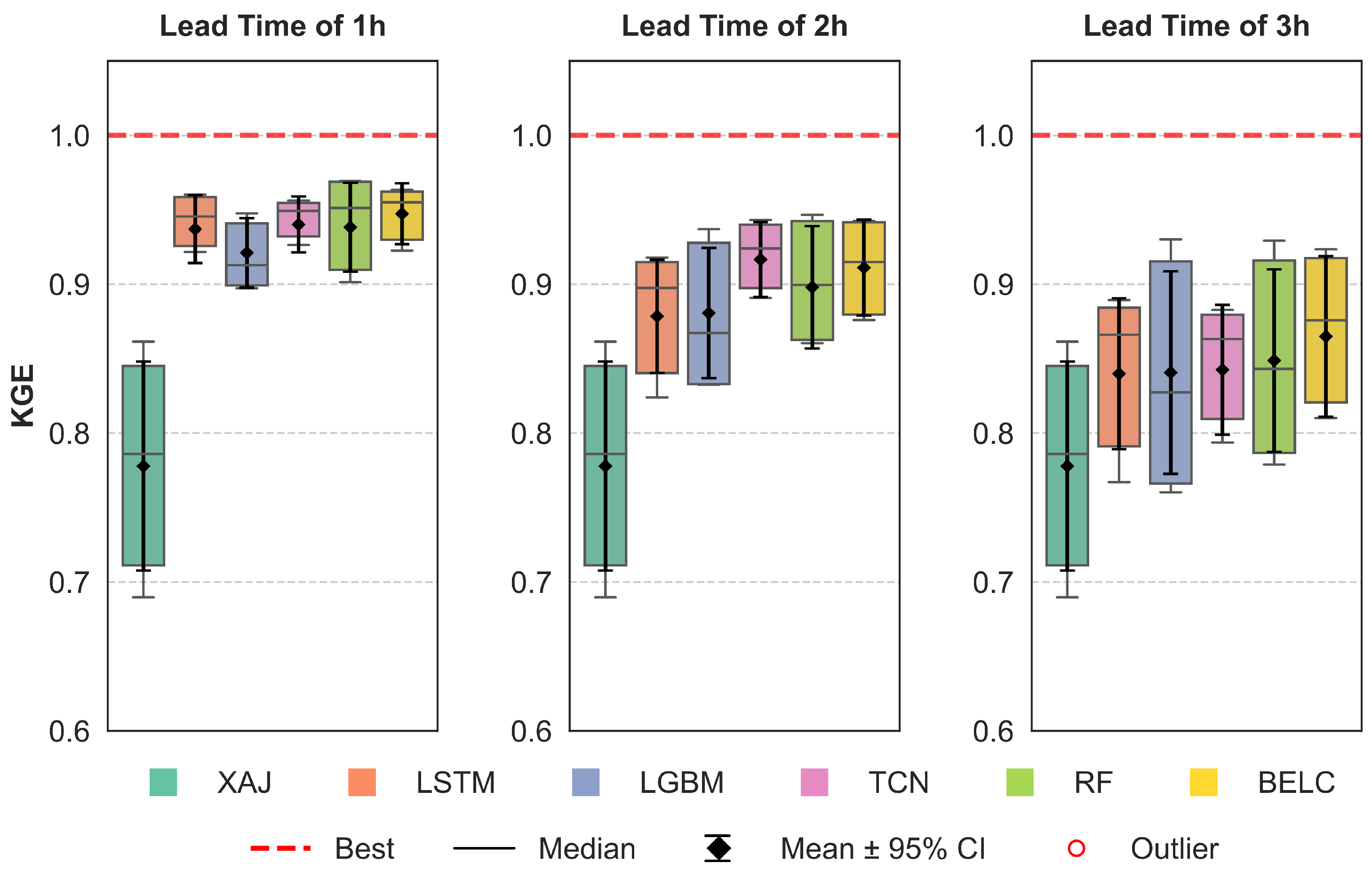
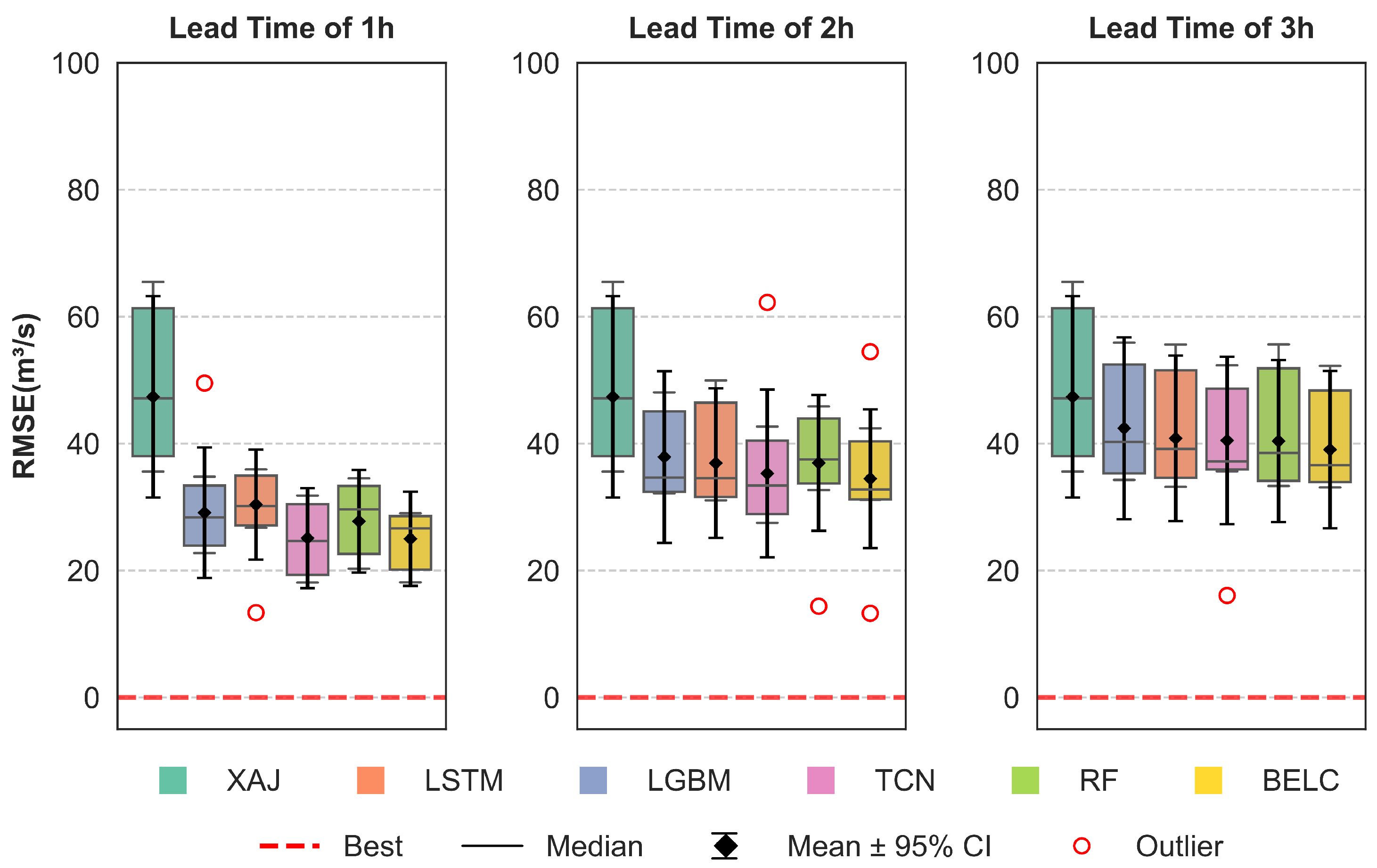
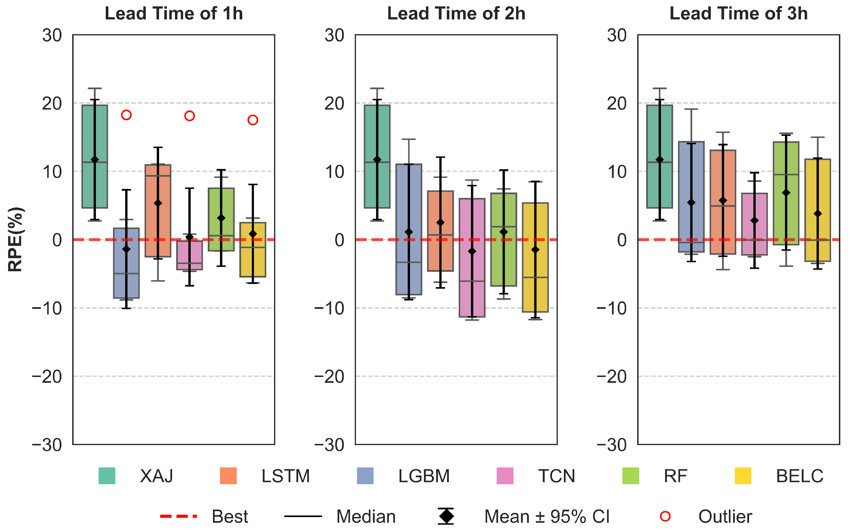
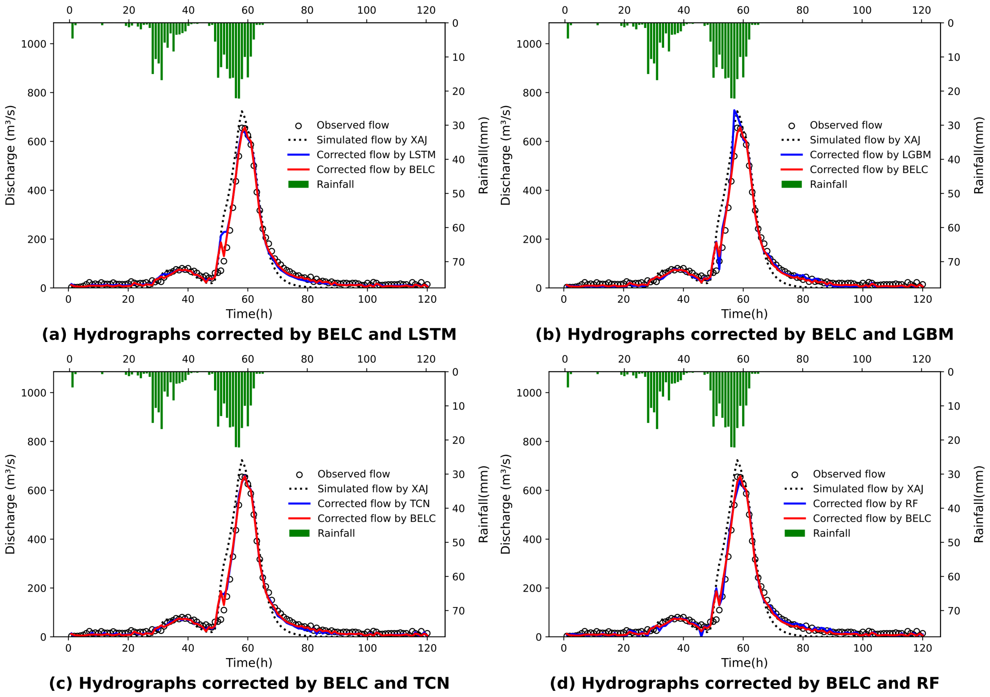
All four baseline schemes can effectively correct flood errors and improve forecasting performance for all lead times, but their performance varies across different lead times and specific flood events. No single machine learning method can maintain optimal robustness and correction effectiveness for all lead time scenarios.

ii. 

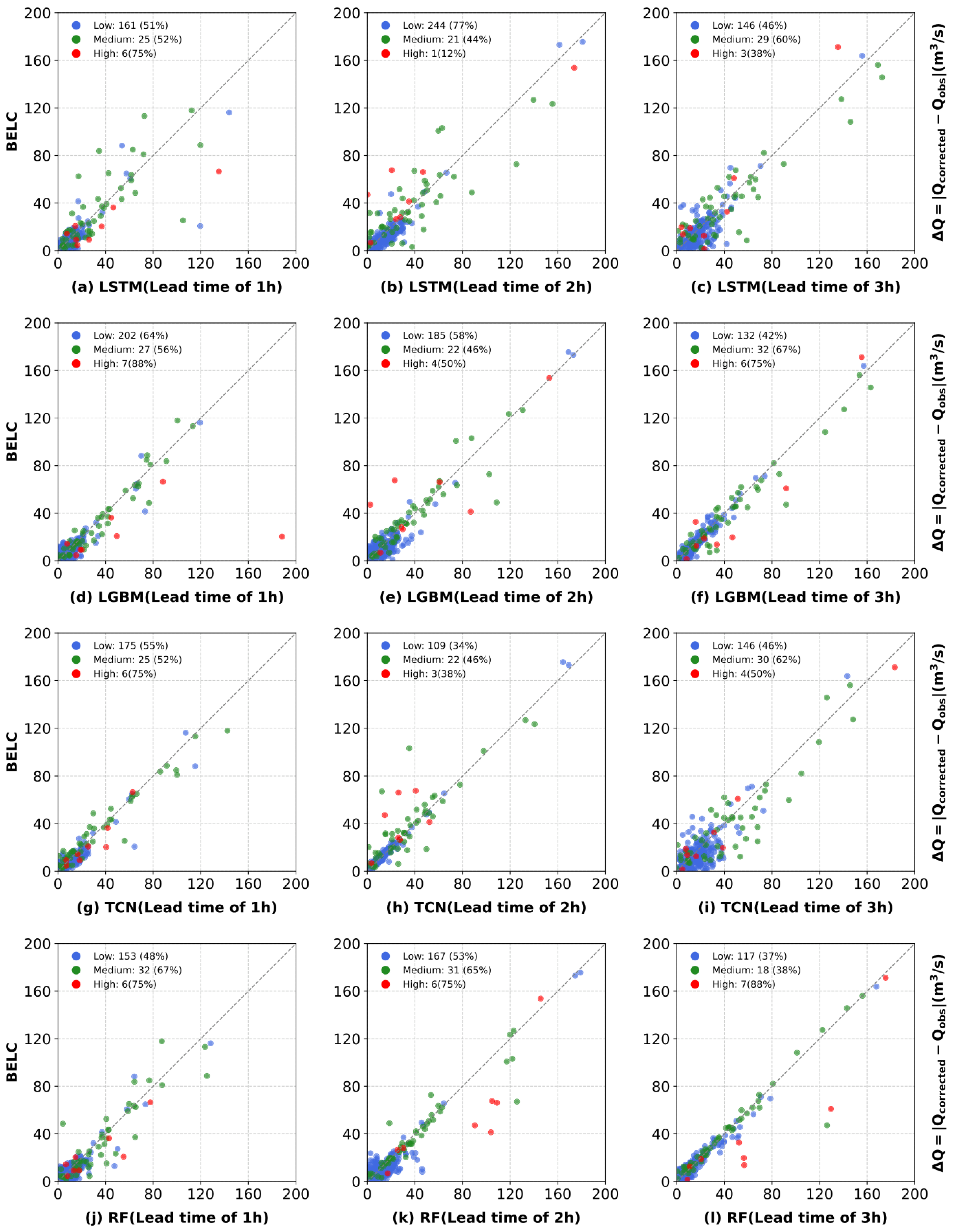
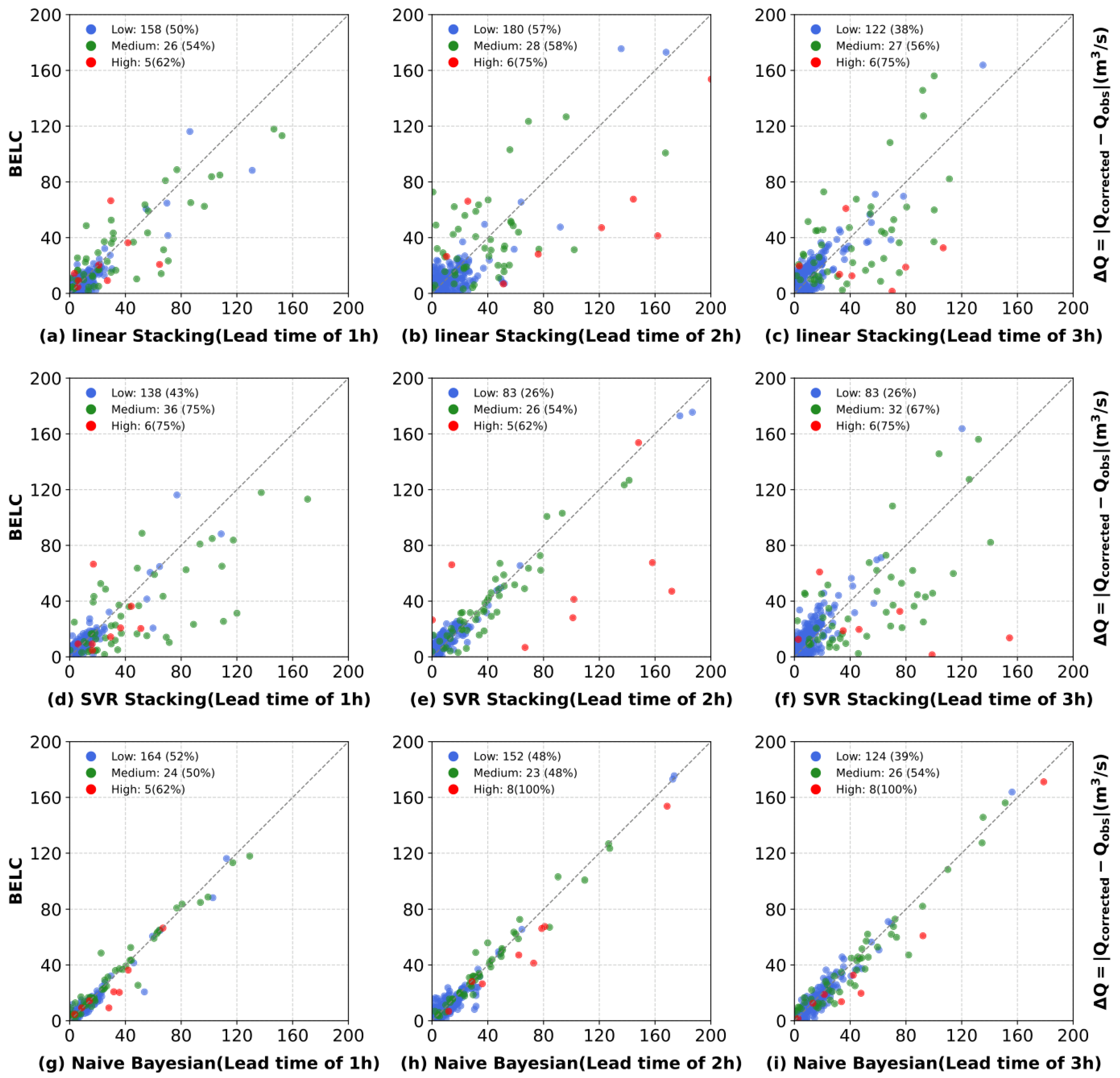
The BELC scheme exhibited superior error correction capability and demonstrated robust performance across 1–3 h lead times, outperforming both baseline schemes and conventional ensemble learning approaches. Evaluated across five metrics (NSE, KGE, RMSE, RPE, and PTE), the BELC outperformed other models in most scenarios. The average performance metrics of the validation period were 0.95 (NSE), 0.92 (KGE), 24.25 ${\mathrm{m}}^3$/s (RMSE), and 8.71% (RPE), with a PTE consistently below 1 h in advance. Meanwhile, BELC maintained stable correction performance across varying flow ranges, delivering reliable flood flow forecasts with outstanding comprehensive performance.

iii.

The K-means flow range clustering significantly enhanced the BELC model’s adaptability to various types of flood, substantially improving flood flow correction accuracy for high flow ranges. The correction performance surpassed that of the Naive Bayesian scheme by 62%, 100%, and 100% for a lead time of 1, 2, and 3 h, respectively.

In practical implementation, the BELC scheme can be integrated into existing hydrological forecasting systems based on the XAJ model. The computational routine follows a “Preprocessing → Data Assimilation → Correction” workflow: (1) Input: Initial forecast results from traditional hydrological models; (2) Data Assimilation: The latest observed runoff, evapotranspiration, and rainfall data is collected from hydrological stations to form a supervised training set, combined with the initial forecast results; (3) Correction: The BELC scheme adjusts the initial forecast results based on the assimilated data.

Building on the improvements achieved by the BELC scheme, future work could focus on the following directions: (1) fusing radar rainfall forecasts and satellite remote sensing data to extend the lead time of real-time correction; (2) investigating the clustering effects of different K values and different baseline machine learning methods; (3) enhancing uncertainty quantification for the BELC scheme; (4) extending the applicability of the BELC scheme through integration with distributed and physical hydrological models (for example, SWAT, VIC, etc.).

References

1. Peredo, D.; Ramos, M.H.; Andréassian, V.; Oudin, L. Investigating hydrological model versatility to simulate extreme flood events. Hydrol. Sci. J. 2022, 67, 628–645. [Google Scholar] [CrossRef]
2. Xin, Z.; Shi, K.; Wu, C.; Wang, L.; Ye, L. Applicability of Hydrological Models for Flash Flood Simulation in Small Catchments of Hilly Area in China. Open Geosci. 2019, 11, 1168–1181. [Google Scholar] [CrossRef]
3. Ren-Jun, Z. The Xinanjiang model applied in China. J. Hydrol. 1992, 135, 371–381. [Google Scholar] [CrossRef]
4. Zotz, G.; Thomas, V. How Much Water is in the Tank? Model Calculations for Two Epiphytic Bromeliads. Ann. Bot. 1999, 83, 183–192. [Google Scholar] [CrossRef]
5. Beven, K. TOPMODEL: A critique. Hydrol. Processes 1997, 11, 1069–1085. [Google Scholar] [CrossRef]
6. Abbott, M.; Bathurst, J.; Cunge, J.; O’Connell, P.; Rasmussen, J. An introduction to the European Hydrological System—Systeme Hydrologique Europeen, “SHE”, 1: History and philosophy of a physically-based, distributed modelling system. J. Hydrol. 1986, 87, 45–59. [Google Scholar] [CrossRef]
7. Liang, X.; Lettenmaier, D.P.; Wood, E.F. One-dimensional statistical dynamic representation of subgrid spatial variability of precipitation in the two-layer variable infiltration capacity model. J. Geophys. Res. Atmos. 1996, 101, 21403–21422. [Google Scholar] [CrossRef]
8. Arnold, J.G.; Srinivasan, R.; Muttiah, R.S.; Williams, J.R. Large Area Hydrologic Modeling and Assessment Part I: Model Development. JAWRA J. Am. Water Resour. Assoc. 1998, 34, 73–89. [Google Scholar] [CrossRef]
9. Ko, D.; Lee, T.; Lee, D. Spatio-temporal-dependent errors of radar rainfall estimates in flood forecasting for the Nam River Dam basin. Meteorol. Appl. 2018, 25, 322–336. [Google Scholar] [CrossRef]
10. Shen, Y.; Ruijsch, J.; Lu, M.; Sutanudjaja, E.H.; Karssenberg, D. Random forests-based error-correction of streamflow from a large-scale hydrological model: Using model state variables to estimate error terms. Comput. Geosci. 2022, 159, 105019. [Google Scholar] [CrossRef]
11. Shi, P.; Wu, H.; Qu, S.; Yang, X.; Lin, Z.; Ding, S.; Si, W. Advancing real-time error correction of flood forecasting based on the hydrologic similarity theory and machine learning techniques. Environ. Res. 2024, 246, 118533. [Google Scholar] [CrossRef] [PubMed]
12. Huang, Y.; Wang, Q.; Liang, Z.; Deng, X. Research advances on real-time correction methods for flood forecasting. South-North Water Transf. Water Sci. Technol. 2021, 19, 12–35. [Google Scholar] [CrossRef]
13. Zhang, T.; Liang, Z.; Bi, C.; Wang, J.; Hu, Y.; Li, B. Statistical Post-Processing for Precipitation Forecast Through Deep Learning Coupling Large-Scale and Local-Scale Spatiotemporal Information. Water Resour. Manag. 2025, 39, 145–160. [Google Scholar] [CrossRef]
14. Yang, S.; Cheng, R.; Yan, W.; Zhang, Q. Application of Ridge Estimation Method of Rainfall Error BasedDifferential Response in Flood Forecasting of Jianyang Basin. Water Resour. Power 2023, 41, 1–3+58. [Google Scholar] [CrossRef]
15. Guo, W.D.; Chen, W.B.; Chang, C.H. Error-correction-based data-driven models for multiple-hour-ahead river stage predictions: A case study of the upstream region of the Cho-Shui River, Taiwan. J. Hydrol. Reg. Stud. 2023, 47, 101378. [Google Scholar] [CrossRef]
16. Wang, W.; Zhao, Y.; Xu, D.; Hong, Y. Error correction method based on deep learning for improving the accuracy of conceptual rainfall-runoff model. J. Hydrol. 2024, 643, 131992. [Google Scholar] [CrossRef]
17. Zounemat-Kermani, M.; Batelaan, O.; Fadaee, M.; Hinkelmann, R. Ensemble machine learning paradigms in hydrology: A review. J. Hydrol. 2021, 598, 126266. [Google Scholar] [CrossRef]
18. Duan, Y.; Liang, Z.; Zhao, J.; Qiu, Z.; Li, B. Combined Forecasting of Hydrological Model Based on Stacking Integrated Framework. Water Resour. Power 2022, 40, 27–30+39. [Google Scholar] [CrossRef]
19. Lin, Y.; Du, Y.; Meng, Y.; Xie, H.; Wang, D. The Influence of Different Integrated Models on Short-term Runoff Forecast in Small Watershed. China Rural. Water Hydropower 2021, 11, 97–102. [Google Scholar]
20. Shin, S.; Her, Y.; Muñoz-Carpena, R.; Khare, Y.P. Multi-parameter approaches for improved ensemble prediction accuracy in hydrology and water quality modeling. J. Hydrol. 2023, 622, 129458. [Google Scholar] [CrossRef]
21. Mohammed, A.; Kora, R. A comprehensive review on ensemble deep learning: Opportunities and challenges. J. King Saud Univ.-Comput. Inf. Sci. 2023, 35, 757–774. [Google Scholar] [CrossRef]
22. Xu, C.; Zhong, P.A.; Zhu, F.; Yang, L.; Wang, S.; Wang, Y. Real-time error correction for flood forecasting based on machine learning ensemble method and its uncertainty assessment. Stoch. Environ. Res. Risk Assess. 2022, 37, 1557–1577. [Google Scholar] [CrossRef]
23. Wolpert, D.H. Stacked generalization. Neural Netw. 1992, 5, 241–259. [Google Scholar] [CrossRef]
24. Lange, H.; Sippel, S. Machine Learning Applications in Hydrology. In Forest-Water Interactions; Springer International Publishing: Cham, Switzerland, 2020; pp. 233–257. [Google Scholar] [CrossRef]
25. Lu, M. Recent and future studies of the Xinanjiang Model. J. Hydraul. Eng. 2021, 52, 432–441. [Google Scholar] [CrossRef]
26. Qiao, X.; Peng, T.; Sun, N.; Zhang, C.; Liu, Q.; Zhang, Y.; Wang, Y.; Nazir, M.S. Metaheuristic evolutionary deep learning model based on temporal convolutional network, improved aquila optimizer and random forest for rainfall-runoff simulation and multi-step runoff prediction. Expert Syst. Appl. 2023, 229, 120616. [Google Scholar] [CrossRef]
27. Kedam, N.; Tiwari, D.K.; Kumar, V.; Khedher, K.M.; Salem, M.A. River stream flow prediction through advanced machine learning models for enhanced accuracy. Results Eng. 2024, 22, 102215. [Google Scholar] [CrossRef]
28. Hochreiter, S.; Schmidhuber, J. Long Short-Term Memory. Neural Comput. 1997, 9, 1735–1780. [Google Scholar] [CrossRef]
29. Li, B.; Li, R.; Sun, T.; Gong, A.; Tian, F.; Khan, M.Y.A.; Ni, G. Improving LSTM hydrological modeling with spatiotemporal deep learning and multi-task learning: A case study of three mountainous areas on the Tibetan Plateau. J. Hydrol. 2023, 620, 129401. [Google Scholar] [CrossRef]
30. Zhang, Y.; Gu, Z.; Thé, J.; Yang, S.; Gharabaghi, B. The Discharge Forecasting of Multiple Monitoring Station for Humber River by Hybrid LSTM Models. Water 2022, 14, 1794. [Google Scholar] [CrossRef]
31. Meng, Q. LightGBM: A Highly Efficient Gradient Boosting Decision Tree. In Proceedings of the Neural Information Processing Systems, Long Beach, CA, USA, 4–9 December 2017. [Google Scholar]
32. Bian, L.; Qin, X.; Zhang, C.; Guo, P.; Wu, H. Application, interpretability and prediction of machine learning method combined with LSTM and LightGBM-a case study for runoff simulation in an arid area. J. Hydrol. 2023, 625, 130091. [Google Scholar] [CrossRef]
33. Gan, M.; Pan, S.; Chen, Y.; Cheng, C.; Pan, H.; Zhu, X. Application of the Machine Learning LightGBM Model to the Prediction of the Water Levels of the Lower Columbia River. J. Mar. Sci. Eng. 2021, 9, 496. [Google Scholar] [CrossRef]
34. Xu, Y.; Hu, C.; Wu, Q.; Li, Z.; Jian, S.; Chen, Y. Application of temporal convolutional network for flood forecasting. Hydrol. Res. 2021, 52, 1455–1468. [Google Scholar] [CrossRef]
35. Breiman, L. Random Forests. Mach. Learn. 2001, 45, 5–32. [Google Scholar] [CrossRef]
36. Singh, A.K.; Kumar, P.; Ali, R.; Al-Ansari, N.; Vishwakarma, D.K.; Kushwaha, K.S.; Panda, K.C.; Sagar, A.; Mirzania, E.; Elbeltagi, A.; et al. An Integrated Statistical-Machine Learning Approach for Runoff Prediction. Sustainability 2022, 14, 8209. [Google Scholar] [CrossRef]
37. Zhou, P.; Xu, Y.; Zhou, X.; Liu, L.; Liang, X.; Guo, Y. Seasonal Streamflow Ensemble Forecasting Based on Multi-Model Fusion. Adv. Sci. Technol. Water Resour. 2025, 45, 62–69. [Google Scholar]
38. Liu, L.; Liang, X.; Wang, Q.; Xu, Y. Justified ERRlS Real-time Correction Method for Streamflow Forecasting Based on Deep Learning. Water Resour. Prot. 2024, 40, 155–164. [Google Scholar]
39. Wu, H.; Shi, P.; Qu, S.; Yang, X.; Zhang, H.; Wang, L.; Ding, S.; Li, H.; Lu, M.; Qiu, C. A hydrologic similarity-based parameters dynamic matching framework: Application to enhance the real-time flood forecasting. Sci. Total Environ. 2024, 907, 167767. [Google Scholar] [CrossRef]
40. McMillan, H.K. A review of hydrologic signatures and their applications. WIREs Water 2021, 8, e1499. [Google Scholar] [CrossRef]
41. Zhang, X.; Song, S.; Guo, T. Nonlinear Segmental Runoff Ensemble Prediction Model Using BMA. Water Resour. Manag. 2024, 38, 3429–3446. [Google Scholar] [CrossRef]
42. Gui, Z.; Zhang, F.; Yue, K.; Lu, X.; Chen, L.; Wang, H. Identifying and Interpreting Hydrological Model Structural Nonstationarity Using the Bayesian Model Averaging Method. Water 2024, 16, 1126. [Google Scholar] [CrossRef]
43. Snoek, J.; Larochelle, H.; Adams, R.P. Practical Bayesian optimization of machine learning algorithms. In Proceedings of the 26th International Conference on Neural Information Processing Systems, Lake Tahoe, NU, USA, 3–6 December 2012; NIPS’12. Volume 2, pp. 2951–2959. [Google Scholar]
44. Gupta, H.V.; Kling, H.; Yilmaz, K.K.; Martinez, G.F. Decomposition of the mean squared error and NSE performance criteria: Implications for improving hydrological modelling. J. Hydrol. 2009, 377, 80–91. [Google Scholar] [CrossRef]
45. GB/T 22482-2008; Standard for Hydrological Information and Forecasting. Standards Press of China: Beijing, China, 2008.
46. Asurza Véliz, F.; Lavado, W. Regional Parameter Estimation of the SWAT Model: Methodology and Application to River Basins in the Peruvian Pacific Drainage. Water 2020, 12, 3198. [Google Scholar] [CrossRef]
Figure 1. Overview of the Hengshan Reservoir Catchment and spatial distribution of precipitation gauges.
Water 17 02048 g001
Figure 2. Preprocessing of the BELC scheme.
Water 17 02048 g002
Figure 3. Workflow of the BELC scheme.
Water 17 02048 g003
Figure 4. Simulated and observed hydrographs of the typical flood events: (a) FN-20190808, (b) FN-20210722, (c) FN-20220912, (d) FN-20230726.
Water 17 02048 g004
Figure 5. Comparison of the NSE of the XAJ model, baseline schemes, and the BELC scheme for the validation period.
Water 17 02048 g005
Figure 6. Comparison of the KGE of the XAJ model, baseline schemes, and the BELC scheme for the validation period.
Water 17 02048 g006
Figure 7. Comparison of the RMSE of the XAJ model, baseline schemes, and the BELC scheme for the validation period.
Water 17 02048 g007
Figure 8. Comparison of the RPE of the XAJ model, baseline schemes, and the BELC scheme for the validation period.
Water 17 02048 g008
Figure 9. Comparison of the PTE of the XAJ model, baseline schemes, and the BELC scheme for the validation period.
Water 17 02048 g009
Figure 10. Comparison of corrected hydrographs of FN-20220912 for baseline schemes and the BELC scheme.
Water 17 02048 g010
Figure 11. Comparison of the the correction effect of the BELC and four baseline schemes for different flow ranges.
Water 17 02048 g011
Figure 12. Comparison of the correction effect between the BELC and three ensemble learning-based schemes for different flow ranges.
Water 17 02048 g012