Incorporation of Horizontal Aquifer Flow into a Vertical Vadose Zone Model to Simulate Natural Groundwater Table Fluctuations

Abstract

The main goal of our work was to evaluate approaches for modeling lateral outflow from shallow unconfined aquifers in a one-dimensional model of vertical variably-saturated flow. The HYDRUS-1D model was modified by implementing formulas representing lateral flow in an aquifer, with linear or quadratic drainage functions describing the relationship between groundwater head and flux. The results obtained by the modified HYDRUS-1D model were compared to the reference simulations with HydroGeoSphere (HGS), with explicit representation of 2D flow in unsaturated and saturated zones in a vertical cross-section of a strip aquifer, including evapotranspiration and plant water uptake. Four series of simulations were conducted for sand and loamy sand soil profiles with deep (6 m) and shallow (2 m) water tables. The results indicate that both linear and quadratic drainage functions can effectively capture groundwater table fluctuations and soil water dynamics. HYDRUS-1D demonstrates notable accuracy in simulating transient fluctuations but shows higher variability near the surface. The study concludes that both quadratic and linear drainage boundary conditions can effectively represent horizontal aquifer flow in 1D models, enhancing the ability of such models to simulate groundwater table fluctuations.

1. Introduction

Subsurface flow models that integrate processes occurring in the unsaturated (vadose) and saturated (groundwater) zones are increasingly applied in water management, including groundwater recharge estimation, determination of irrigation strategies, and evaluation of contaminant fate and transport. Previous studies [1,2,3,4,5,6,7,8,9,10] have shown the importance of this integration, providing explanations for regional and temporal recharge variations. In studying vadose zone contamination originating from polluted surface water, Sasidharan et al. [11] have emphasized its potential consequences, specifically the subsequent pollution of groundwater aquifers. This environmental hazard poses a significant threat to aquatic ecosystems and human health. Implementing managed aquifer recharge (MAR) strategies is a promising solution for enhancing or maintaining the availability of groundwater resources [12,13]. This approach aims to optimize water storage within aquifers, increasing water supply resilience during droughts [14,15]. Integrated saturated–unsaturated water flow models are valuable tools for assessing the feasibility of MAR and associated risks of aquifer contamination.

Subsurface water flow is commonly described using an extended form of the Richards equation (RE), which covers both unsaturated and saturated conditions [2]. The 3D RE formulation is the basis of several comprehensive hydrological models, such as HydroGeoSphere (HGS) [16,17], CATHY [18], ParFlow [19], HYDRUS [20], and MIKE SHE [21,22]. In some of these models, RE is coupled with equations describing surface water flow to form a complete representation of the land hydrological cycle [16,18,21]. However, such models are characterized by large complexities and computational demands, which limit their applicability, especially for larger spatial scales.

On the other hand, simplified models of vadose zone flow based on a 1D form of RE describing vertical flow found widespread application in hydrology and related fields, including estimation of groundwater recharge [10,23,24,25], evaluation of climate change effects [9,26,27,28], prediction of contaminant fate [29,30,31,32,33], and simulation of MAR operations [12,13]. Several numerical codes to simulate 1D vadose zone processes are freely available (e.g., HYDRUS-1D [34,35], SWAP [34,35]) and have extensive capabilities to simulate contaminant transport or plant–soil–atmosphere interactions, which are not always available in multidimensional integrated hydrological models. Several coupling schemes have been proposed between 1D unsaturated zone numerical codes and multi-layered groundwater modeling software, e.g., the HYDRUS package for MODFLOW [24,36,37,38] or HMSE [39]. However, these couplings remain complex and computationally demanding.

If 1D vertical models are to be used as standalone tools, a question arises about how to account for the effects of groundwater table (GWT) fluctuations and groundwater flow in aquifers, which are typically horizontal. This is especially important for modeling contaminants’ fate [40,41]. Moreover, unsaturated zone models require a significant number of parameters that may be difficult to obtain, which results in increased uncertainty [42,43,44]. In order to provide meaningful results, vadose zone models must be calibrated and validated against field measurements [45]. GWT measurements are a good alternative for vadose zone data or evapotranspiration (ET) measurements because they are simpler to obtain and usually more readily available. However, if groundwater levels are used as calibration data, the 1D vertical model of vadose zone flow must be able to reproduce the observed GWT fluctuations, which requires an appropriate choice of the bottom boundary condition (BC).

In vadose zone flow simulations, the bottom BC is often formulated as (i) a constant or time-variable pressure head corresponding to the measured position of the GWT, (ii) a no-flow BC (impermeable layer), or (iii) free drainage, where the bottom outflow (recharge) is driven by gravity, with the vertical pressure head gradient equal to zero [46]. However, none of these BCs adequately represent horizontal discharge from the soil profile, which is especially important for shallow aquifers discharging to nearby surface waters. If the water table elevation varies rapidly with time, using a pressure head-based BC (i) can lead to unphysical water fluxes at the model bottom (whenever the bottom pressure head changes) and does not represent the natural sequence of GWT fluctuations resulting from infiltration and ET [47]. If a no-flow BC (ii) is used, the influence of lateral groundwater flow is neglected, which is unrealistic for many shallow groundwater systems. When a free drainage BC (iii) is used, the bottom of the modeled soil profile is above the groundwater table; thus, the information about the groundwater level is not included in the model.

Three additional BCs are available to represent lateral outflow from the vertical soil profile and the resulting water table fluctuations in 1D models: (i) a relationship between water flux and GWT position derived from analytical formulas describing flow to drains, (ii) adding an artificial soil layer at the bottom of the profile, and (iii) an exponential relationship between water flux and GWT level. They seem to be used much less often than the pressure head-based or free drainage BCs, and we describe them in more detail below. The first possibility is to use analytical formulas describing flow to drains, such as the Hooghoudt equation [35,48]. They provide an estimate of water flux as a function of the position of the water table in the soil profile and the nearby drain and thus constitute a system-dependent boundary condition. The calculated flux can be applied as a BC in the bottom node of the soil profile or distributed among all nodes below the groundwater table. The SWAP manual [49] describes how to use this approach to represent aquifer flow in vadose zone models. However, practical applications of this approach in case studies are limited. Gumuła-Kawęcka et al. [23] used a similar approach to reproduce vadose zone–groundwater interactions for a shallow outwash plain aquifer surrounded by lakes. Applying measured GWT positions as an additional calibration criterion improved the modeling results compared with simulations where only soil water content measurements were used. For that purpose, Gumuła-Kawęcka et al. [23] used a simple equation describing flow to drains implemented in HYDRUS-1D, where the flux is proportional to the difference of the squares of water table levels in the soil profile and the nearby water body (a quadratic drainage BC). Gumuła-Kawęcka et al. [27] used the calibrated 1D model to evaluate the influence of long-term climate change effects on groundwater table levels in outwash plain aquifers. In another study [26], which considered lateral outflow in the 1D model, it was possible to forecast GWT levels and recharge in a sandbar aquifer affected by rising sea levels until 2100. One advantage of using drain flow formulas is that they are physically based. In simple hydrological settings, the parameters of the drainage equation (e.g., the horizontal conductivity of the aquifer or the distance to a drain) can be directly estimated. However, in more complex hydrosystems, actual flow patterns in the aquifer may differ from those assumed by the drainage equation, and its parameters must be fitted.

Lateral water flow between the soil profile and the neighboring surface water body can also be represented by adding a layer of fictitious soil material at the bottom of the soil profile, below the range of expected GWT fluctuations [50]. The boundary condition is specified in terms of the water pressure head at the bottom of the added layer, which corresponds to the position of the water table in the external water body. The hydraulic conductivity and thickness of the added layer are adjusted so that the resistance to flow provided by the layer is the same as the resistance to aquifer flow between the soil profile and the surface water body. For example, Vonk [50] added a 2-cm-thick soil layer with a hydraulic conductivity of 0.0427 cm/day at the bottom of soil profiles in HYDRUS-1D simulations to investigate GWT fluctuations caused by time-variable recharge for a variety of soil textures. This is equivalent to specifying a system-dependent boundary condition, where the drainage flux is proportional to the difference between the GWT level in the profile and the external reservoir. The two water levels are considered in the first power (a linear drainage BC), not the second power (a quadratic drainage BC), as in the drain flow equations for an unconfined aquifer. Note that a similar boundary condition is commonly used in groundwater modeling to represent flow to/from distant boundaries (e.g., the GHB package in MODFLOW or the “fluid transfer” condition in HGS).

The third option to represent groundwater flow from the soil profile is given by an exponential relationship between the outflow from the soil profile and the GWT level. This formula was introduced by Hopmans and Stricker [51] and later implemented into HYDRUS-1D (a “deep drainage” BC). It was also applied as a bottom boundary condition in 1D models by Neto et al. [52], Corona et al. [53,54], and Brunner and Simmons [53,54]. Hopmans and Stricker [51] showed that the exponential formula reasonably approximates the relationship between the GWT level and groundwater outflow at the watershed scale. However, the parameters of this equation do not have a clear physical significance and must be calibrated. Moreover, using the exponential formula, one cannot reproduce an equilibrium state (i.e., no flow) when the GWT level in the soil profile is the same as the water level in the surface body because the formula predicts a non-zero outflow (although decreasing with lowering GWT) for any GWT position. Similarly, it is impossible to predict groundwater flow into the soil profile when the water table in the drain is above the GWT level in the soil profile because, in the exponential formula, the flux has the same direction for GWT above and below the drain water level.

Regardless of the widespread use of 1D vadose zone models, there is still a gap about how well 1D vertical models can capture natural groundwater table fluctuations when lateral aquifer flow takes place. As 1D vertical models do not directly represent this process, 2D and 3D models do. Previous studies have verified 1D models using field data, which includes uncertainty because of measurement errors, unknown aquifer geometry, and subsurface characteristics. Therefore, simulating GWT fluctuations in 1D models with various bottom boundary conditions is difficult.

This study directly fills this gap by:

• Eliminating uncertainties associated with field measurements and aquifer heterogeneity, the performance of HYDRUS-1D models with quadratic and linear drainage boundary conditions is evaluated using reference 2D HGS simulations.
• HYDRUS-1D’s extended quadratic and linear drainage equations are applied and tested to compare them methodically with reference 2D solutions.
• To fully assess model performance under various hydrological conditions, several scenarios that alter soil type, groundwater table depth, and profile position within the catchment are run.

The primary goals of this study are:

i.

To assess the degree to which GWT fluctuations can be accurately reproduced by 1D models with system-dependent drainage boundary conditions as compared to a 2D reference model.

ii.

To compare the simulation results of groundwater movement and unsaturated flow between the HGS and modified HYDRUS-1D models.

iii.

To determine the applicability and limitations of linear and quadratic drainage boundary conditions in 1D vadose zone modeling [16,17].

2. Materials and Methods

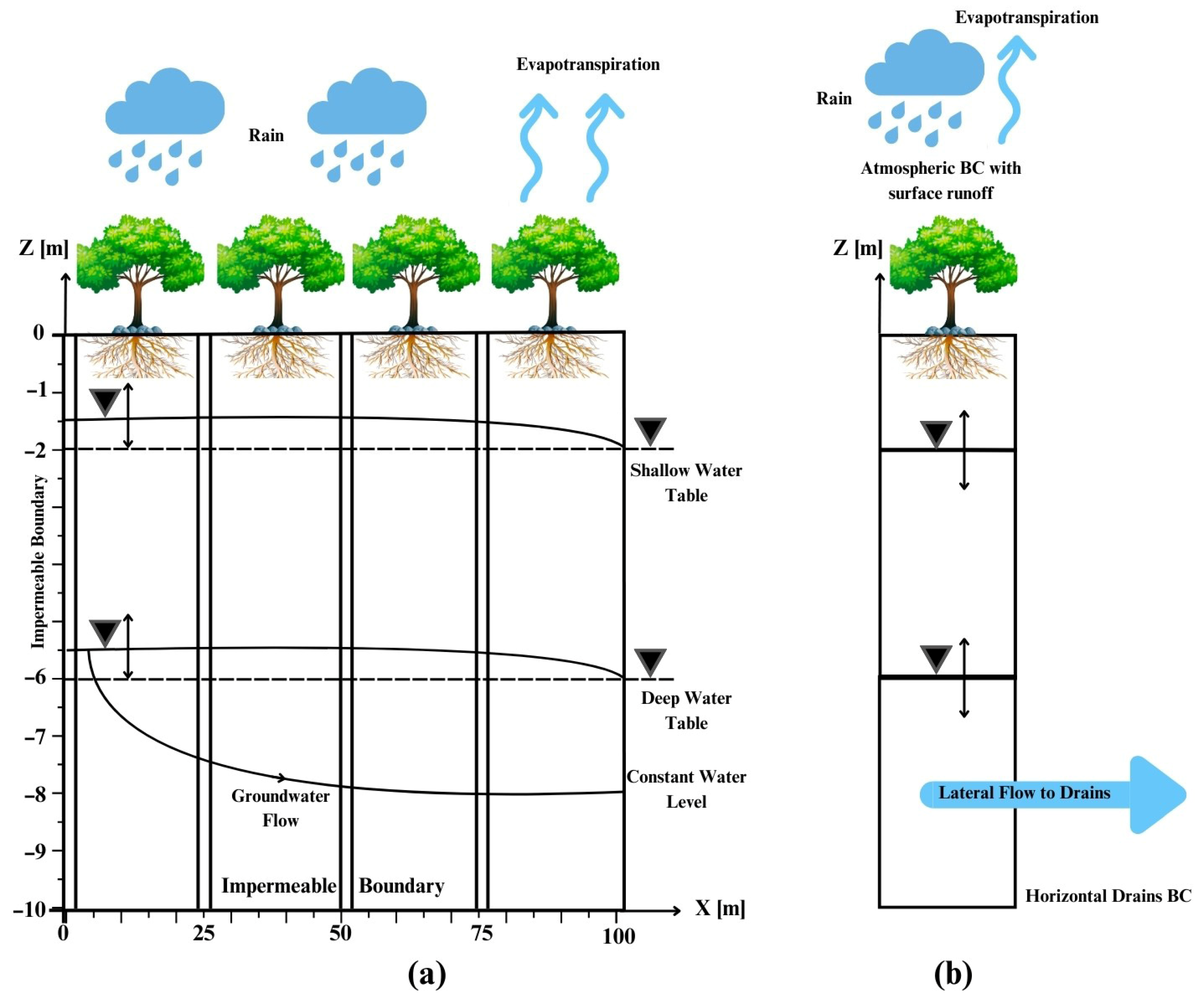
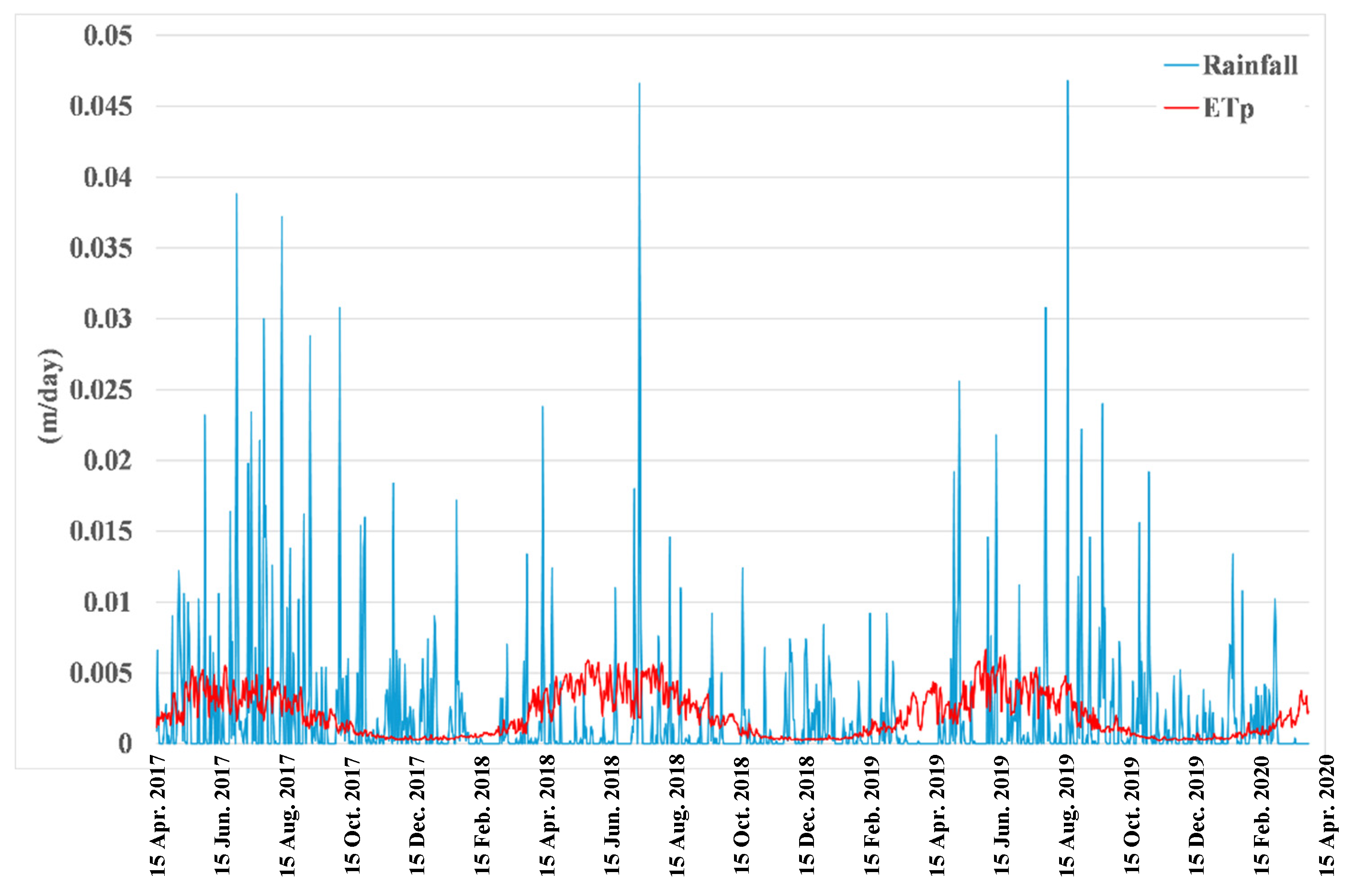
2.1. General Simulation Setup

The conceptual framework for our comparative analysis is illustrated in Figure 1. As a reference case, we consider 2D flow in the vertical cross-section of an unconfined aquifer and an overlying vadose zone (Figure 1a). The subsurface domain is homogeneous and isotropic and consists of either sand or loamy sand, depending on the considered scenario. The flow is driven by atmospheric fluxes (precipitation and evapotranspiration, ET) along the upper boundary (ground surface). The bottom and left boundaries are impermeable. A constant head BC is imposed on the right side, representing perfect hydraulic contact with an external surface water body. The surface water level is constant in time and determines the reference level for GWT fluctuations. Simulations were performed for a shallow GWT, where the surface water level is at a depth of 2 m, and a deep GWT, with the surface water level at a depth of 6 m (Figure 1). Four series of simulations were carried out: (i) sandy soil with the surface water table at 6 m (denoted SA_6m), (ii) sandy soil with the surface water table at 2 m (SA_2m), (iii) loamy sand with the surface water table at 6 m (LS_6m), and (iv) loamy sand with the surface water table at 2 m (LS_2m). To observe pressure head and water content distributions along the vadose zone profile, four monitoring points were situated at depths of 0 m, 1 m, 2 m, and 7 m.

GWT fluctuations calculated by the HGS model (Version 20140807) at specific x coordinates (x = 0, x = 50 m) (Figure 1a) were compared to the results of 1D simulations performed in HYDRUS-1D (Version 4.14) (Figure 1b), assuming parameters consistent with a 2D model. The bottom BC in the 1D model was specified using either quadratic or linear drainage equations (the corresponding models are labeled H1D_1 and H1D_2, respectively). In all simulation series, we included both evaporation and transpiration processes. For the SA_6m series, we additionally performed one simulation without evapotranspiration and root water uptake and one with evaporation only (i.e., without transpiration or root water uptake). We also performed a basic verification of the models through steady-state simulations.

In the reference 2D HGS simulations, the right-hand boundary was implemented as a constant head to represent hydraulic contact with a surface water body (e.g., a river or a lake), while the bottom and left boundaries were set as impermeable, allowing explicit simulation of both vertical and lateral groundwater flow. In contrast, HYDRUS-1D, which is limited to vertical flow, used a system-dependent drainage boundary at the bottom of the profile. This was implemented as either a quadratic or linear drainage function, both of which relate groundwater head to outflow rate and are well-established methods for representing lateral discharge in 1D models. These approaches ensure that the simulated groundwater table fluctuations in HYDRUS-1D remain physically consistent and comparable to the 2D HGS reference, as demonstrated in recent applications [23,49,50].

2.2. HGS Simulations

The two-dimensional flow simulations were performed using HGS [55], a completely integrated three-dimensional hydrological tool simulating flow processes in the vadose zone, groundwater, and surface water. For unsaturated flow in the vadose zone, HGS solves a 3D form of the Richards equation, which, for the case of a non-fractured porous medium, can be written as follows:

$$-\nabla ·\left(q\right)+\sum r_{ex}\pm Q={\displaystyle \frac{\mathsf{\partial }}{\mathsf{\partial }t}}({\theta }_s·S_w)$$

(1)

where $q$ represents the fluid flux $\left[L T^{-1}\right]$, $r_{ex }$ signifies the volumetric fluid exchange rate $\left[L^3 L^{-3} T^{-1}\right]$ with other flow domains (in our case, surface water), $Q$ is a sink/source term (volumetric fluid flux per unit volume) $\left[L^3 L^{-3} T^{-1}\right]$, ${\theta }_s$ denotes the saturated volumetric water content [-], and $S_w$ is the water saturation [-]. The van Genuchten-Mualem [56] model was used for soil hydraulic properties:

$$\theta \left(h\right)={\theta }_r+{\displaystyle \frac{{\theta }_s-{\theta }_r}{{\left[1+{\left(\mathsf{\alpha }\left|h\right|\right)}^n\right]}^{-m}}}$$

(2a)

$$K\left(S_e\right)=K_s·K_r=K_s·S_e^{\tau }·{\left[1-{\left(1-S_e^{1/m}\right)}^m\right]}^2$$

(2b)

where $\theta \left(h\right)$ represents the soil water retention curve $\left[L^3 L^{-3}\right]$, ${\theta }_r$ is the residual volumetric water content [-], ${\theta }_s$ is the saturated soil water content [-], $\mathsf{\alpha }$ is the average pore size $\left[L^{-1}\right]$, $h$ is the pressure head $\left[L\right]$, $n$ and $m$ are related to the pore-size distribution [-] with $m=1-{\displaystyle \frac{1}{n}},$ $K$ is the unsaturated hydraulic conductivity $\left[L T^{-1}\right]$, $S_e$ is the effective saturation [-] equal to ${\displaystyle \frac{\theta -{\theta }_r}{{\theta }_s-{\theta }_r}}$, $K_s$ is the saturated hydraulic conductivity $\left[L T^{-1}\right]$, $K_r$ is the relative hydraulic conductivity [-], and $\tau$ is a parameter related to pore tortuosity and connectivity [-]. We assigned parameters of van Genuchten functions for sand and loamy sand based on Carsel and Parrish [57] (

Table 1. Soil hydraulic parameters used in the HGS and HYDRUS-1D simulations based on Carsel and Parrish [57].

Soil Material	θr [-]	θs [-]	α [1/m]	n [-]	m [-]	Ks [m/d]	τ [-]
Sand	0.045	0.43	14.5	2.68	0.627	7.128	0.5
Loamy Sand	0.057	0.41	12.4	2.28	0.570	3.502	0.5

). The specific storage parameter $S_s$ ${[L}^{-1}]$, which is not shown explicitly in Equation (1) but is used in the approximation of the storage term, was equal to 0.00001 ${\mathrm{m}}^{-1}$ in all scenarios. Equation (1) was solved on a rectangular numerical grid consisting of 2222 nodes, 4110 faces, and 1000 elements, corresponding to the dimensions of 100 m by 10 m by 1 m (note that HGS is fully 3D, so a quasi-2D model was built by setting a single layer of cells in y direction).

The potential evapotranspiration (ET_P $\left[L T^{-1}\right]$) was calculated using the Penman–Monteith model [58] with a constant LAI of 2. Daily meteorological data for the simulations (2017–2020) (Figure 2) were obtained from measurements in the experimental field in Cekcyn (N53.54, E17.97) conducted by Gdańsk University of Technology [23]. Data for the warm-up simulations (2014–2017) were provided by the Chojnice weather station (N53.71, E17.53) operated by the Institute of Meteorology and Water Management—National Research Institute, Poland. Potential evapotranspiration was divided into transpiration and evaporation fluxes. In the absence of interception, root water uptake in HGS is calculated as follows:

$$S=f_1\left(LAI\right)f_2\left(\theta \right) RDF\left(z\right){ET}_p$$

(3a)

where $S$ represents the root water uptake intensity $\left[ T^{-1}\right]$, $f_1\left(LAI\right)$ is the leaf area index function [-], $f_2\left(\theta \right)$ represents the nodal water content function [-], and $RDF$ is the time-varying root distribution function $\left[ L^{-1}\right]$. The $f_1$ and $f_2\left(\theta \right)$ functions are further expressed as:

$$f_1\left(LAI\right)=\max \left\{0, min\left[1, \left(C_2+C_1 LAI\right)\right]\right\}$$

(3b)

$$f_2\left(\theta \right)=\left\{\begin{array}{c}\begin{array}{c}\begin{array}{c}0 for 0\le \theta \le {\theta }_{wp}\\ 1-{\left[{\displaystyle \frac{{\theta }_{fc}-\theta }{{\theta }_{fc}-{\theta }_{wp}}}\right]}^{C_3} for {\theta }_{wp}\le \theta \le {\theta }_{fc}\\ 1 for {\theta }_{fc}\le \theta \le {\theta }_o\end{array}\\ 1-{\left[{\displaystyle \frac{{\theta }_{an}-\theta }{{\theta }_{an}-{\theta }_o}}\right]}^{C_3} for {\theta }_o\le \theta \le {\theta }_{an}\end{array}\\ 0 for {\theta }_{an}\le \theta \end{array}\right.$$

(3c)

where $C_1$ = 0.30, $C_2$ = 0.20, and $C_3$ = 1. The parameters $C_1$ and $C_2$ were chosen in such a way that the factor $f_1$, describing the partitioning of ${ET}_p$ between potential transpiration and potential evaporation, has a value of 0.803, which is the same as the corresponding partitioning coefficient in HYDRUS-1D simulations (see Equation (6a)). The transpiration limiting water contents [-], i.e., the wilting point (${\theta }_{wp}$), field capacity (${\theta }_{fc}$), oxic limit (${\theta }_o$), and anoxic limit (${\theta }_{an}$) were calculated separately for sand and loamy sand using the van Genuchten (1980) model [56] (Equation (2a)) to correspond with the transpiration limiting pressure heads in the Feddes et al. (1978) model [59] applied in HYDRUS (see Equation (6c)).

In HGS, the evaporation flux is distributed over a user-specified depth below the soil surface. To maintain consistency with HYDRUS-1D simulations, where evaporation flux is applied only in the surface node, we assumed a low evaporation depth of 0.03 m in the HGS model. The evaporation intensity per unit evaporation depth, E_S, was calculated as follows:

$$E_S={\mathsf{\alpha }}^{*}\left({ET}_P-E_{OLF}\right)\left(1-f_1\left(LAI\right)\right)EDF$$

(4a)

$${\mathsf{\alpha }}^{*}=\left\{\begin{array}{c}{\displaystyle \frac{\theta -{\theta }_e}{{\theta }_{e1}-{\theta }_{e2}}} for {\theta }_{e2}\le \theta \le {\theta }_{e1}\\ 1 for {\theta >\theta }_{e1}\\ 0 for {\theta <\theta }_{e2}\end{array}\right.$$

(4b)

where ${\mathsf{\alpha }}^{*}$ is a wetness factor, E_OLF is evaporation from surface water (negligible in our simulations), and $EDF$ is the evaporation distribution function, assumed to be quadratically decreasing with depth. The evaporation limiting water contents ${\theta }_{e1}$ and ${\theta }_{e2}$ were equal to 0.32 and 0.2, respectively.

While surface water flow was included in the HGS simulations, surface runoff was negligible since we considered highly permeable soils in our scenarios. For this reason, we do not provide details on surface flow modeling here.

2.3. HYDRUS-1D Simulations

HYDRUS-1D [48] simulations are based on the 1D Richards equation describing vertical flow:

$${\displaystyle \frac{\mathsf{\partial }\theta \left(h\right)}{\mathsf{\partial }t}}={\displaystyle \frac{\mathsf{\partial }}{\mathsf{\partial }z}}\left(k\left(h\right){\displaystyle \frac{\mathsf{\partial }h}{\mathsf{\partial }z}}\right)+{\displaystyle \frac{\mathsf{\partial }k\left(h\right)}{\mathsf{\partial }z}}-S\left(h\right)$$

(5)

where $\theta$ is the volumetric water content $\left[L^3 L^{-3}\right]$, $h$ is the water pressure head $\left[L\right]$, $t$ is time $\left[T\right]$, $z$ is the spatial coordinate $\left[L\right]$ (positive in the upward direction), $k$ is the unsaturated hydraulic conductivity function $\left[L T^{-1}\right]$, and $S$ is a sink term $\left[L^3 L^{-3} T^{-1}\right]$ representing root water uptake (RWU).

The 10 m deep soil profile was discretized with 404 uniformly spaced nodes. The soil hydraulic properties and initial conditions in 1D simulations were consistent with the parameters used in 2D HGS simulations. The upper boundary condition was specified as an atmospheric condition with instantaneous surface runoff. In HYDRUS-1D, root water uptake (S) is calculated as follows:

$$S=f_1\left(LAI\right)f_2\left(h\right) RDF\left(z\right){ET}_p$$

(6a)

where

$$f_1\left(LAI\right)=1-e^{-k\ast LAI}$$

(6b)

$$f_2(h)=\left\{\begin{array}{c}0 h\ge h_1, h\le h_4\\ {\displaystyle \frac{h-h_1}{h_2-h_1}} h_2\le h<h_1\\ 1 { h}_3<h\le h_2\\ {\displaystyle \frac{h-h_4}{h_3-h_1}} h_4<h\le h_3\end{array}\right.$$

(6c)

where $k=0.463$ is the default value of the extinction coefficient, $h_1$ is the anaerobiosis point pressure head $\left[L\right]$, and $h_4$ is the wilting point pressure head $\left[L\right]$. Root water uptake $S$ is equal to zero if the soil is wetter than the anaerobiosis point $\left(h\ge h_1\right)$ or dryer than the wilting point $(h\le h_4)$. Root water uptake increases between $h_4$ and $h_3$, from $h_3$ to $h_2$ it has a maximal value, and decreases between $h_2$ and $h_1$. The actual transpiration rate is obtained by integrating root water uptake across the entire root zone.

The pressure heads that limit transpiration correspond to the values reported for pasture by Wesseling et al. [60] (

Table A1. Parameters used in root water uptake calculations in HYDRUS-1D and HydroGeoSphere.

HydroGeoSphere			HYDRUS-1D
Parameters of the Transpiration Function [-]	Sand	Loamy Sand	Feddes Model Parameters (m)
Wilting point (θwp)	0.105	0.139	Anaerobiosis point pressure head (h1)	−0.25
Field capacity (θfc)	0.107	0.151	Upper pressure head limit of maximum root uptake (h2)	−2
Oxic limit (θo)	0.205	0.329	Lower pressure head limit of root uptake increase (h3)	−8
Anoxic limit (θan)	0.498	0.634	Wilting point pressure head (h4)	−80
Residual saturation (Swr)	0.1046	0.1390

—Appendix A). RDF linearly decreases to a depth of 1 m, as in HGS simulations. The evaporation model in HYDRUS-1D also differs from the one in HGS. Potential evaporation is calculated as follows:

$$E={ET}_P\ast \left(1-f_1\left(LAI\right)\right)$$

(7)

and applied as the boundary flux in the surface node. The evaporation flux is limited by the condition $h_{surf}>h_{crit}$, where $h_{surf}$ is the water pressure head at the surface node and $h_{crit}$ is the water pressure head corresponding to the relative air humidity. We assumed constant $h_{crit}=-10 \mathrm{m}$ in all simulations.

We implemented two variants of the drainage equation as additional options in the “Horizontal drains” BC in HYDRUS. The quadratic equation is based on the Hooghoudt analytical solution for flow to uniformly spaced trenches fully penetrating the aquifer [61]:

$$q_{dr}={\displaystyle \frac{4K_{dr}}{L_{dr}^2}} \left(H^2-H_{dr}^2\right)=CD1 \left(H^2-H_{dr}^2\right)$$

(8)

where $q_{dr}$ is the drainage flux $\left[L T^{-1}\right]$, $K_{dr}$ is the horizontal hydraulic conductivity of the aquifer $\left[L T^{-1}\right]$, $L_{dr}$ is the spacing between the drains $\left[L \right]$, $H$ is the groundwater table elevation above the aquifer bottom $\left[L \right]$, and $H_{dr}$ is the water table in the drain (trench) above the aquifer bottom $\left[L \right]$. ${\displaystyle \frac{4K_{dr}}{L_{dr}^2}}$ can be combined into a single parameter—conductance $CD1$ [(m*s)⁻¹]. Note that in the current standard version of HYDRUS-1D, the Hooghoudt equation is implemented in a slightly different form, describing flow to a drain with a small circular cross-section lying on an impermeable soil layer. Equation (8) is valid for the soil profile located at the water divide in the middle between drains, i.e., at x = 0 in our setting. For this case, $CD1$ can be calculated directly. For the profiles located at other x coordinates, we considered $CD1$ as a fitting parameter and adjusted it manually to obtain the best possible agreement with the reference HGS solution.

The linear equation is given as:

$$q_{dr}=CD2 \left(H-H_{dr}\right)$$

(9)

where the conductance $CD2$ has dimension of [s⁻¹]. The linear equation is strictly valid for flow in confined aquifers, and in that case, $CD2$ can be calculated theoretically. In our study, we calibrated $CD2$ manually to obtain the best possible fit with the HGS solution.

2.4. Convergence Analysis

To confirm our results are not influenced by the choice of spatial discretization, we conducted a detailed convergence analysis using the SA_6m x at 0 m scenario with actual weather conditions for both HYDRUS-1D and HGS models. We ran a series of simulations with gradually coarser and refined meshes, precisely using 101, 202, 404 (baseline mesh), 606, and 808 nodes in HYDRUS-1D models and corresponding block counts in the Z-axis in HGS. For each configuration, we compared the simulated groundwater table fluctuations against those from the baseline mesh, using root mean square error (RMSE) as our main indicator, together with the mean, range, and standard deviation (

Table A2. Summary statistics of the convergence analysis.

Mesh/Scenario	Model	Min (m)	Max (m)	Range (m)	Mean (m)	Std Dev (m)	RMSE vs. Finest (m)
SA_6m with 101 nodes	H1D_1	−6	−5.761	0.239	−5.927	0.0674	0.0347
	H1D_2	−6	−5.765	0.235	−5.929	0.0659	0.0345
	HGS	−6.027	−5.767	0.26	−5.942	0.073	0.0924
SA_6m with 202 nodes	H1D_1	−5.985	−5.742	0.243	−5.909	0.0695	0.0165
	H1D_2	−5.985	−5.747	0.238	−5.911	0.068	0.0163
	HGS	−6.035	−5.775	0.26	−5.949	0.0743	0.0945
SA_6m with 404 nodes	H1D_1	−5.978	−5.731	0.247	−5.894	0.0725	0
	H1D_2	−5.978	−5.736	0.242	−5.897	0.0709	0
	HGS	−6	−5.741	0.259	−5.913	0.0746	0
SA_6m with 606 nodes	H1D_1	−5.992	−5.744	0.248	−5.911	0.0722	0.0178
	H1D_2	−5.992	−5.749	0.243	−5.914	0.0707	0.0177
	HGS	−6.025	−5.764	0.261	−5.939	0.0727	0.0914
SA_6m with 808 nodes	H1D_1	−5.999	−5.75	0.249	−5.918	0.0728	0.0238
	H1D_2	−5.999	−5.755	0.244	−5.92	0.0712	0.0238
	HGS	−6.024	−5.763	0.261	−5.938	0.0723	0.0901

). The RMSE values between the standard and finest discretizations were consistently below 0.04 m in HYDRUS-1D, and similarly low in HGS, confirming that our results are effectively mesh independent. This systematic approach to grid refinement and quantitative error assessment is in line with the best practices recommended by Kabala & Milly [62,63,64], who emphasize the importance of demonstrating numerical convergence in hydrological modeling.

2.5. Sensitivity Analysis

To understand how much our results depend on uncertainty in key soil parameters, a one-at-a-time sensitivity analysis was carried out, focusing on the saturated hydraulic conductivity (Ks) in both HYDRUS-1D and HGS. For this analysis, we systematically increased and decreased Ks by 10% and 20% from its baseline value of 7.128, while keeping all other model settings unchanged. For each scenario, we recalculated the RMSE, mean, and range of groundwater table fluctuations relative to the baseline simulation (

Table A3. Summary statistics of the sensitivity analysis.

Parameter/Scenario	Model	Min (m)	Max (m)	Range (m)	Mean (m)	Std Dev (m)	RMSE vs. Baseline (m)
SA_6m with −10 Ks	H1D_1	−5.978	−5.731	0.247	−5.896	0.0723	0.0031
	H1D_2	−5.978	−5.736	0.242	−5.898	0.0705	0.0032
	HGS	−6	−5.741	0.259	−5.913	0.0746	0
SA_6m with −20 Ks	H1D_1	−5.978	−5.732	0.246	−5.897	0.0724	0.0064
	H1D_2	−5.978	−5.736	0.242	−5.9	0.0706	0.0064
	HGS	−6	−5.741	0.259	−5.913	0.0746	0
SA_6m with baseline Ks	H1D_1	−5.978	−5.731	0.247	−5.894	0.0725	0
	H1D_2	−5.978	−5.736	0.242	−5.897	0.0709	0
	HGS	−6	−5.741	0.259	−5.913	0.0746	0
SA_6m with +10 Ks	H1D_1	−5.978	−5.73	0.248	−5.893	0.0726	0.0028
	H1D_2	−5.978	−5.735	0.243	−5.896	0.0703	0.0028
	HGS	−6	−5.741	0.259	−5.913	0.0746	0
SA_6m with +20 Ks	H1D_1	−5.978	−5.73	0.248	−5.893	0.0719	0.0052
	H1D_2	−5.978	−5.735	0.243	−5.896	0.0703	0.0051
	HGS	−6	−5.741	0.259	−5.913	0.0746	0

). The results show that changing Ks within this range had only a small effect on groundwater table fluctuations. Both models maintained an RMSE below 0.01 m when we increased or decreased Ks by 10%. The evidence shows that both HYDRUS-1D and HGS are robust to reasonable uncertainty in Ks and that our results are not sensitive to reasonable modifications in Ks. The sensitivity analysis follows the recommendations of Kabala & Milly [62,63,64], who emphasize the need to change parameters in a systematic way and to assess how the model is sensitive in hydrological modeling.

3. Results and Discussion

3.1. Steady State Simulation SA_6m

The steady-state simulation results for the SA_6m scenario (sandy soil with a surface water level 6 m deep) are presented in

Table 2. Results from the steady-state flow simulations.

Models	Observation Point No (Depth Below the Ground Level)	Pressure Head [m]	Water Content [-]
HYDRUS-1D	1 (0 m)	−0.17	0.12
	2 (2 m)	0.85	0.43
	3 (7 m)	5.86	0.43
HydroGeoSphere	1 (0 m)	−0.16	0.12
	2 (2 m)	0.82	0.43
	3 (7 m)	5.82	0.43

. For the surface node (0 m), the HYDRUS-1D model shows a stable pressure head of approximately −0.17 m, while the HGS model shows a slightly lower value of −0.16 m. At the monitoring points located 2 m and 7 m below the ground level, the HYDRUS-1D model predicts pressure heads of around 0.85 m and 5.86 m, respectively, whereas the HGS model shows values of 0.82 m and 5.82 m. For the volumetric water content, both models gave a consistent value of 0.12 for the surface node and fully saturated conditions (θ = 0.43) for the monitoring points at depths 2 m and 7 m. These results align well with the analytical solution using Hooghoudt’s equation (Equation (8)).

3.2. Simulations SA_6m for the Scenario with Actual Weather Conditions

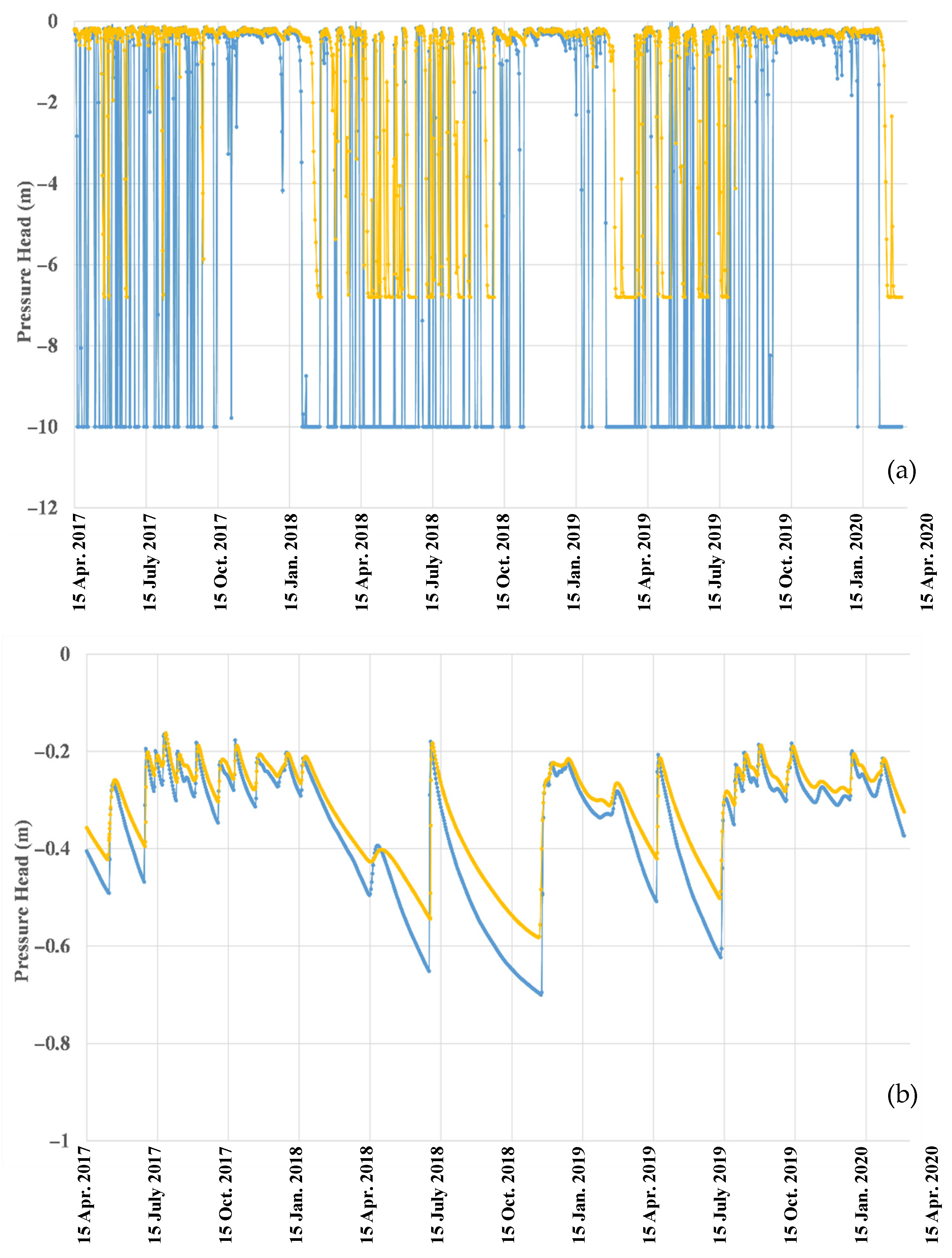
3.2.1. Pressure Heads and Water Table Fluctuations at x = 0 m

Figure 3 presents variations in the GWT level and pressure head distributions within the vertical sandy profile simulated using the HYDRUS-1D (with quadratic or linear drainage equations, H1D_1 ($CD1$ = 200 (m*s)⁻¹) and H1D_2 ($CD2$ = 0.006 s⁻¹), respectively) and HGS (at x = 0 m, representing water divide (see Figure 1)) models. The results of both HYDRUS-1D simulations (with quadratic or linear drainage equations) are consistent and show frequent and rapid changes in the pressure head, especially at the ground surface, where the values range between −10 m and 0 m (Figure 3a). The HGS model predicted smaller pressure head variations, with longer periods of a relatively stable pressure head, with the pressure heads at the ground surface varying between −6.8 m and 0 m (Figure 3a). Similar trends were found for deeper observation points, with the differences between the HYDRUS-1D and HGS results decreasing with depth. The pressure heads 1 m below the ground surface vary between −0.70 and −0.18 m (H1D_1, H1D_2) and −0.58 and −0.18 m (HGS). The pressure heads at a depth of 2 m vary between −0.45 and −0.17 m (H1D_1, H1D_2) and −0.4 and −0.17 m (HGS) (Figure 3b,c). The significant differences in pressure heads close to the land surface computed by HYDRUS-1D and HGS can be explained by the differences in evaporation calculations by the two hydrological models (see Equations (4a) and (7)). However, we note that sandy soils have the same water content for all practical purposes at pressure heads of −6.8 m and −10 m, i.e., closely related to the residual water content of 0.045.

Figure 3d shows groundwater table levels simulated using the HYDRUS-1D and HGS (for x = 0 m) models for actual weather conditions (precipitation and ET_P in Figure 2). All three simulations provided consistent results. The simulated groundwater table depths between April 2017 and April 2020 varied between 5.73 and 5.94 m (simulated by H1D_1), 5.74 and 5.94 m (H1D_2), and 5.74 and 5.96 m (HGS). Starting from relatively low GWT levels (5.82–5.92 m) in April–July 2017, an intensive rise in the GWT level is observed in all simulations during the rainy period between July 2017 and January 2018 [27]. After the peak, which occurred from October 2017 to March 2018, all models show a significant decline in the groundwater level, reaching its minimum between September 2018 and October 2019 due to drought in 2018 [27]. After November 2019, the water table increased due to rainfall in the summer and autumn of 2019.

3.2.2. Pressure Heads and Water Table Fluctuations at x = 50 m

Figure 4 depicts the GWT levels obtained for the soil profile situated in the middle of the watershed, 50 m from the water divide (Figure 1). In this case, the HGS simulation results were compared with the HYDRUS-1D model results with modified drain conductances ($CD1$ = 150 (m*s)⁻¹ for H1D_1 and $CD2$ = 0.011 s⁻¹ for H1D_2) to represent a different distance to the drain. For all three simulations, water table fluctuations show a similar pattern as in the soil profile situated at the water divide (x = 0 m). However, the range of the GWT fluctuations is slightly lower—the GWT depth varies between 5.82 and 5.96 m (H1D_1), 5.83 and 5.96 m (H1D_2), and 5.80 and 5.97 m (HGS). All three models align closely in overall trends and range, with the HYDRUS-1D models presenting more variable fluctuations and the HGS model maintaining smoother transitions. During the recharge periods, the HGS simulation exhibits a higher water table rise, possibly caused by side groundwater inflow in the 2D model.

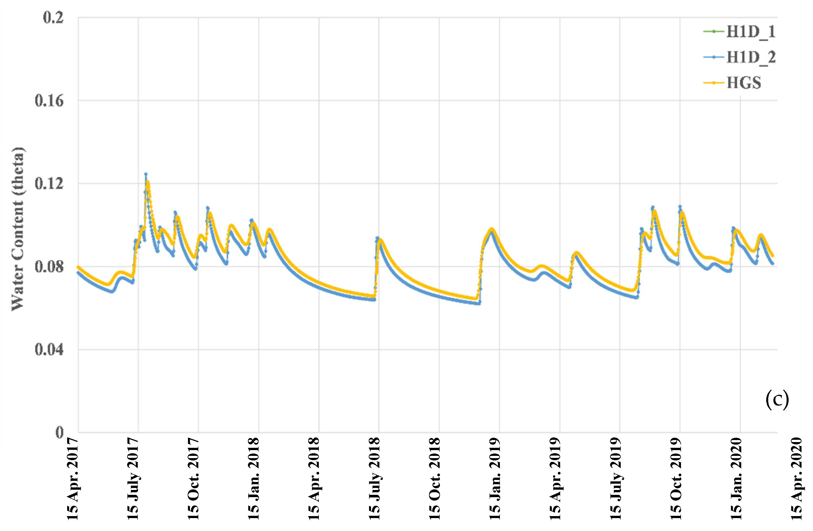
3.2.3. Soil Water Contents

Water contents simulated by the HGS and HYDRUS-1D models were analyzed for three depths: ground surface (0 m), 1 m, and 2 m (Figure 5). The results show the largest variations in the surface node (Figure 5a), which are closely related to individual precipitation events. All three simulations predicted the maximum water content of approximately 0.16 after heavy rainfalls, while the minimum water content of about 0.045 occurred during dry periods. At a depth of 1 m, water contents increased from 0.053 to 0.12 (H1D_1 and H1D_2), and from 0.055 to 0.12 (HGS) (Figure 5b). Similar results were simulated for a depth of 2 m by all three models, between 0.062 and 0.12 (Figure 5c). Water content fluctuations reflect the timing and intensity of precipitation, with clear and frequent changes in response to rainfall events. Water content variations in the 2 m deep soil layer simulated using the HYDRUS-1D and HGS models closely align, demonstrating that both numerical codes are highly reliable for modeling soil moisture dynamics.

3.3. Simulations SA_6m for Scenarios with and Without Evaporation and Transpiration

Figure 6 compares groundwater table fluctuations in the sandy soil profile with the surface water level 6 m deep (i.e., SA_6m) simulated for scenarios (a) neglecting evapotranspiration, (b) considering evaporation and neglecting transpiration, and (c) considering both evaporation and transpiration (root water uptake). Figure 6a provided the highest and most variable water table levels (5.32–5.82 m below the ground level). Figure 6b shows that the consideration of evaporation produced a deeper groundwater table (5.56–5.92 m), with similar fluctuations but slightly lower peaks than in Figure 6a. The additional consideration of plant water uptake in Figure 6c resulted in more uniform, less variable groundwater table levels (5.73–5.96 m).

Several conclusions can be deduced from the results of all scenarios. First, both numerical codes (HYDRUS-1D and HGS) produced closely aligned GWT fluctuations, with minor differences of less than 3 cm. Second, the largest GWT fluctuations occurred in the scenario without ET, indicating that the absence of a vegetation cover resulted in more apparent GWT variations. In contrast, the smallest fluctuations were observed in the scenario that considered both evaporation and plant water uptake, highlighting the root zone’s profound effect on shallow GWT fluctuations. The presence of plants not only reduced the amplitude of GWT fluctuations but also changed their time distribution, suggesting that plant cover influences both the magnitude and time of groundwater response.

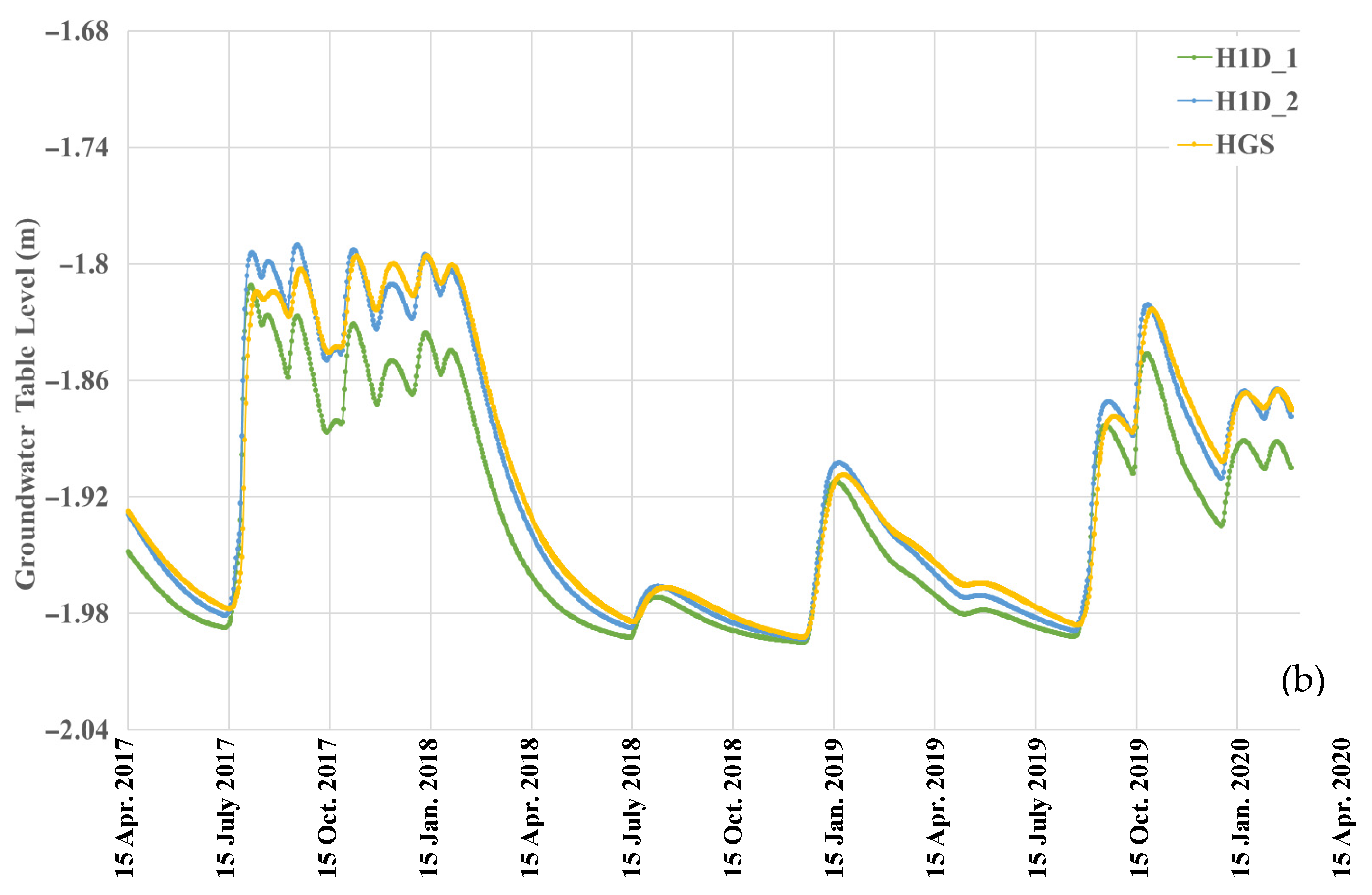
3.4. Simulations SA_2m

Figure 7 shows the GWT fluctuations simulated for the sandy soil profile located at (i) x = 0 m (Figure 1) using the H1D_1 ($CD1$ = 200 (m*s)⁻¹), H1D_2 ($CD2$ = 0.012 s⁻¹), and HGS models, and (ii) x = 50 m using the H1D_1 ($CD1$ = 150 (m*s)⁻¹), H1D_2 ($CD2$ = 0.021 s⁻¹), and HGS models. Setting the surface water level at 2 m resulted in higher groundwater table levels than in simulations SA_6m. In the first case (x = 0 m), the groundwater table depth was simulated using the HYDRUS-1D model between 1.80 and 1.99 m below the ground surface and using the HGS model between 1.77 and 2.00 m. All simulations provided closely aligned time distributions of groundwater level fluctuations (Figure 7a) despite the H1D_1 and H1D_2 models showing slightly lower peaks (3 cm) after the extremely rainy July 2017. Similar differences between the results of the HYDRUS-1D and HGS models were observed for recharge periods for the second profile (x = 50 m). In this case, water table depths ranged between 1.84 and 2.00 m for H1D_1 and H1D_2 and 1.82 and 1.99 m for HGS (Figure 7b).

For both x = 0 m and x = 50 m, the HGS model gave higher peaks and similar minimum GWT levels as the HYDRUS-1D models. The results for the second profile showed a larger range of fluctuations, especially for the HGS model. However, all simulated scenarios provided a similar time series of groundwater level variations and consistently represented water table responses to precipitation.

3.5. Simulations LS_6m

The groundwater levels obtained for loamy sand profiles are presented in Figure 8 for two locations: (i) x = 0 m (Figure 1) simulated using the H1D_1 ($CD1$ = 200 (m*s)⁻¹), H1D_2 ($CD2$ = 0.003 s⁻¹), and HGS models, and (ii) x = 50 m simulated using the H1D_1 ($CD1$ = 150 (m*s)⁻¹), H1D_2 ($CD2$ = 0.051 s⁻¹), and HGS models. In the first case (x = 0 m), all simulations provided similar time distributions of recharge periods and water table depths, about 5.55–5.91 m for HYDRUS-1D and 5.55–5.93 m for HGS (Figure 8a). Larger discrepancies were found in the second case (x = 50 m). The HGS model simulated a maximum GWT level of 5.65 m, while the H1D_1 and H1D_2 models produced slightly lower peaks at 5.70 m and 5.71 m, respectively (Figure 8b). All simulations produced a minimum GWT level of 5.94 m during a dry period with minimal precipitation. Nevertheless, HYDRUS-1D and HGS show similar trends of water table fluctuation, with slight differences in peak values.

The discrepancies between GWT levels obtained by both numerical codes are closely aligned with the results simulated for a deeper sandy profile (Section 3.2). For the soil profile at the water divide (x = 0 m), HGS simulated the groundwater level during dry periods 2 cm lower than HYDRUS-1D. On the contrary, for the profile located 50 m from the water divide, HGS simulated the groundwater table during abundant recharge periods 5 cm higher than HYDRUS-1D.

3.6. Simulations LS_2m

The results for the shallow loamy sand profiles are presented in Figure 9. Simulations were carried out for two locations: (i) the soil profile located at x = 0 m (Figure 1) was simulated using the H1D_1 ($CD1$ = 200 (m*s)⁻¹), H1D_2 ($CD2$ = 0.006 s⁻¹), and HGS models, and (ii) the soil profile at x = 50 m was simulated using the H1D_1 ($CD1$ = 150 (m*s)⁻¹), H1D_2 ($CD2$ = 0.078 s⁻¹), and HGS models. In the first case (x = 0 m), the overall trends in water table fluctuations are closely aligned in all simulations, with groundwater table depths between 1.73 and 1.99 m below the ground level (Figure 9a).

The results are less consistent in the second case (x = 50 m). The differences in GWT levels were up to 5 cm, especially during abundant recharge periods, August 2017–January 2018 and October 2019–April 2020 (Figure 9b). Nevertheless, all simulations provided a similar range of groundwater fluctuations. The lowest water table levels were obtained by H1D_1 (1.81–2.00 m below the ground level), while H1D_2 and HGS gave higher values, 1.79–1.99 m and 1.80–1.99 m, respectively. While the range of the results is higher, the changes are smoother and less rapid compared to the shallow sandy profile (Section 3.3). All simulations (H1D_1, H1D_2, and HGS) showed consistent performance with reasonable accuracy in reproducing GWT levels, indicating that either model can effectively capture groundwater dynamics. Additionally, the fluctuation patterns across all models were found to be physically consistent.

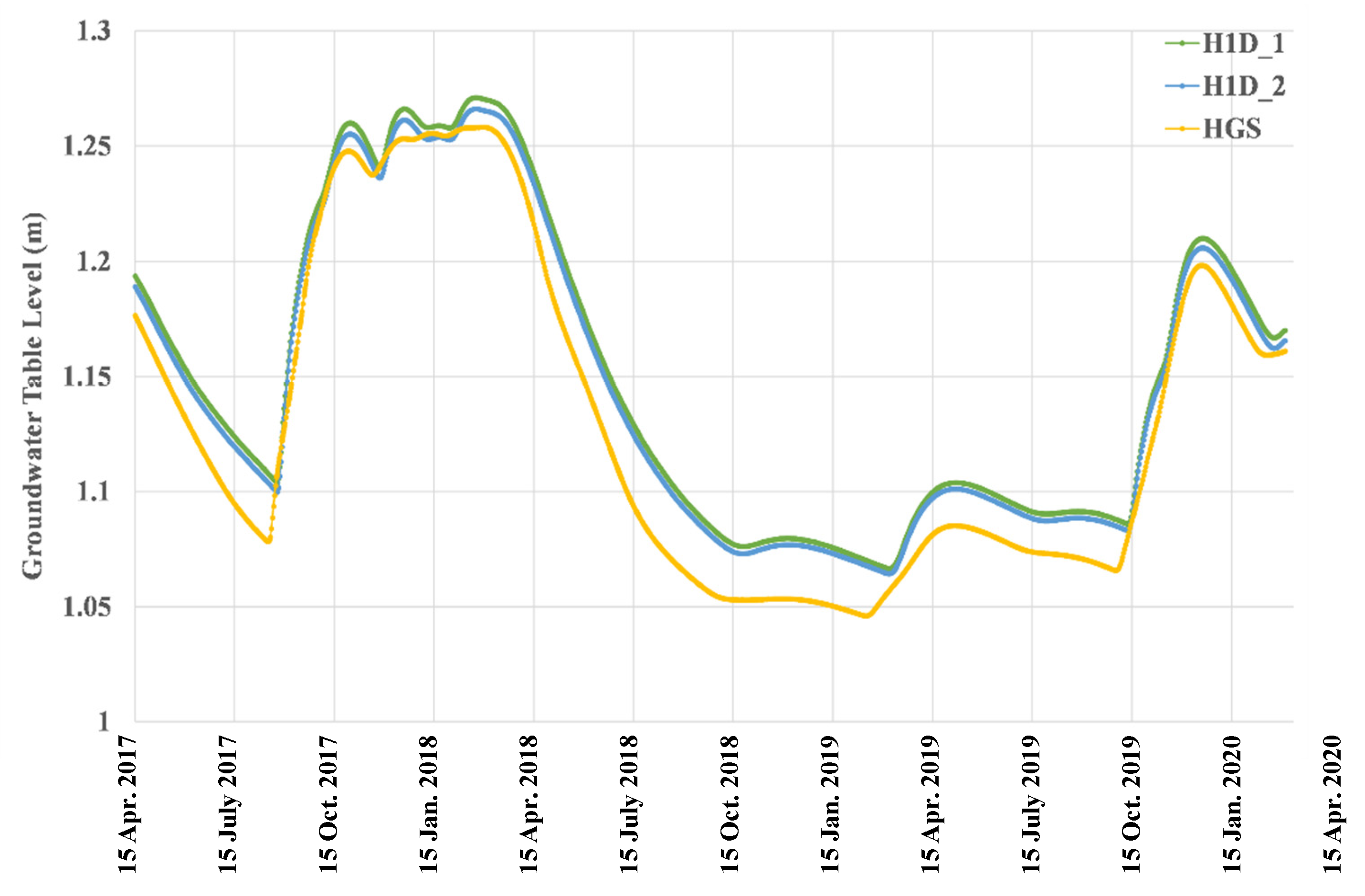
3.7. Simulations with Low Permeability Lens in the Vadose Zone

Figure 10 illustrates the GWT levels for the low permeability lens composed of sandy loam soil in the vadose zone (x = 20–80 m) and sand soil material (SA_6m) in the entire domain, obtained using the H1D_1 (CD1 = 200 (m*s)⁻¹), H1D_2 (CD2 = 0.006 s⁻¹), and HGS models.

In all three simulations, the water table fluctuations exhibit a similar pattern. However, the range of GWT fluctuations is slightly narrower: the GWT varies between 1.06 and 1.27 m for H1D_1, 1.06 and 1.26 m for H1D_2, and 1.04 and 1.25 m for HGS. All three models closely align in terms of overall trends and ranges. The HYDRUS-1D models show more variable fluctuations, while the HGS model demonstrates smoother transitions. During recharge periods, the HGS simulation shows a more pronounced rise in the water table, which may be attributed to side groundwater inflow in the 2D model.

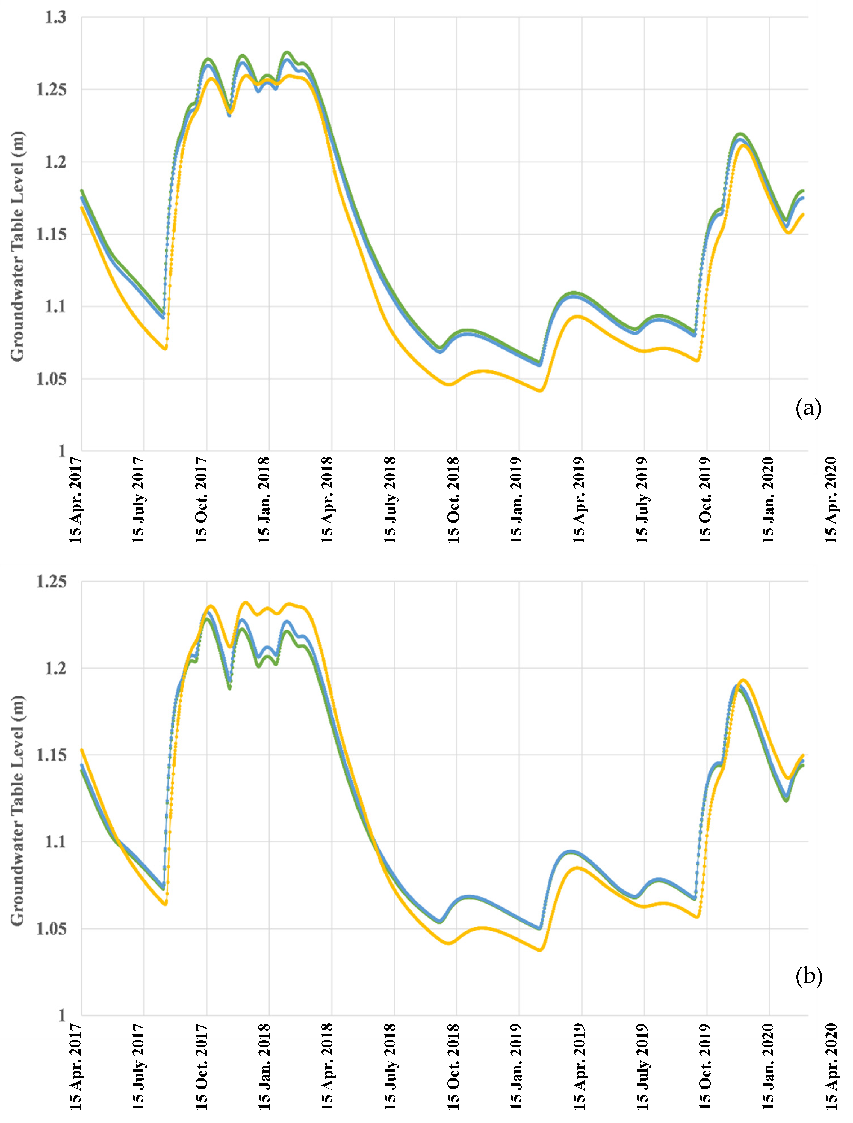
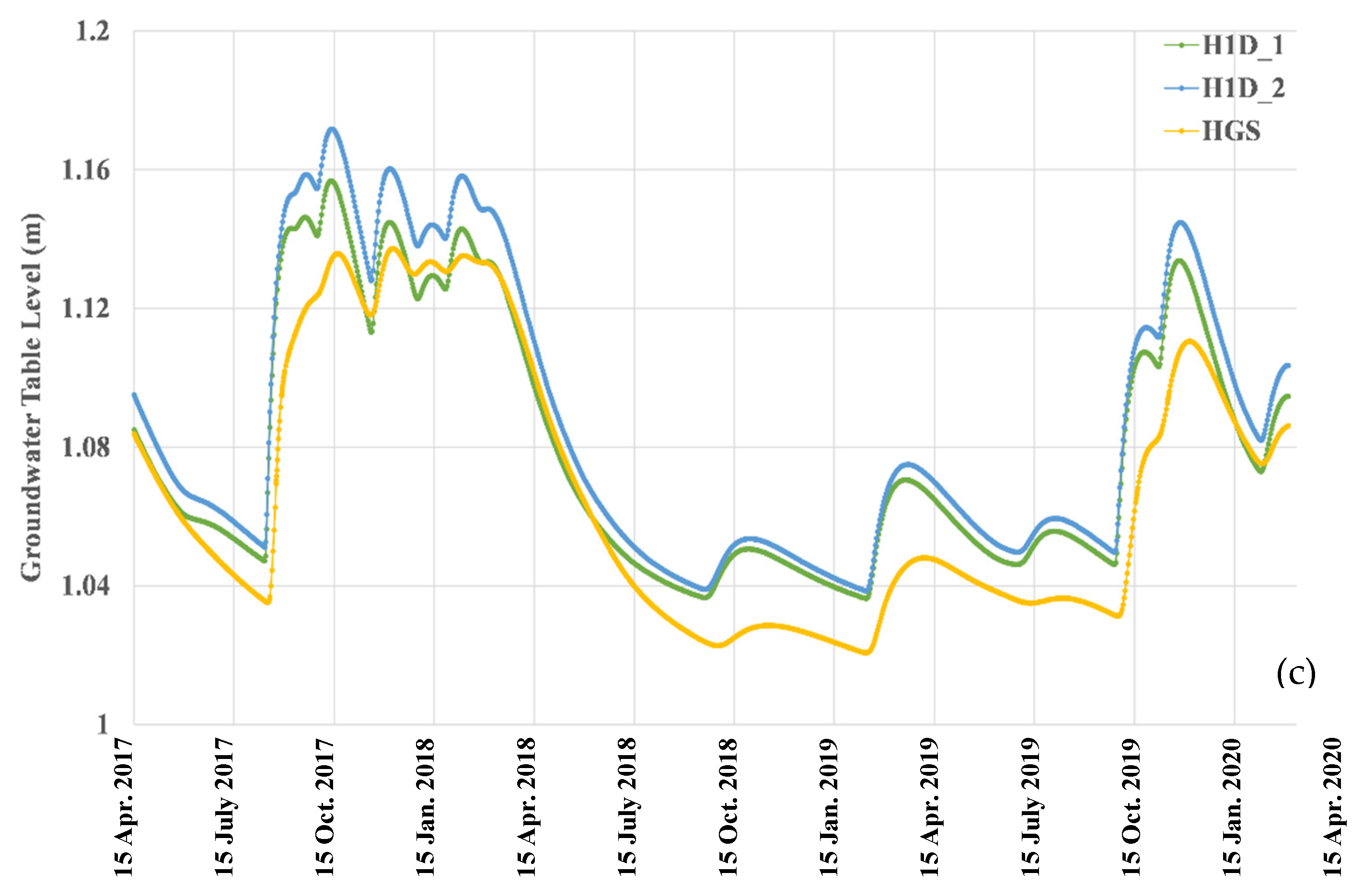
3.8. Simulations with Varying Permeability in Horizontal Direction

Figure 11 compares groundwater table fluctuations in a sandy soil profile with the surface water level at a depth of 6 m (i.e., SA_6m), simulated for varying permeability in the horizontal direction: (i) K1 at x = 0 m with H1D_1 (CD1 = 175 (m*s)⁻¹) and H1D_2 (CD2 = 0.0074 s⁻¹), (ii) K2 at x = 34 m with H1D_1 (CD1 = 200 (m*s)⁻¹) and H1D_2 (CD2 = 0.006 s⁻¹), and (iii) K3 at x = 67 m with H1D_1 (CD1 = 133 (m*s)⁻¹) and H1D_2 (CD2 = 0.0115 s⁻¹).

In the first case (x = 0 m) and the second case (x = 34 m), the overall trends in water table fluctuations are closely aligned across all simulations, with groundwater table depths ranging from 1.05 to 1.27 m in the first case and from 1.03 to 1.23 m in the second case (Figure 11a,b). The results are less consistent in the third case (x = 67 m), where GWT levels vary between 1.03 and 1.15 m in H1D_1, 1.03 and 1.17 m in H1D_2, and 1.02 and 1.13 m in HGS (Figure 11c). Nevertheless, all simulations indicate a similar range of groundwater fluctuations. Each simulation (H1D_1, H1D_2, and HGS) demonstrated consistent performance with reasonable accuracy in reproducing GWT levels.

To compare how the HYDRUS-1D and HGS models performed through all scenarios, the results are summarized in

Table A4. Summary statistics of groundwater table fluctuations captured from all scenarios.

Scenario	Model	Min (m)	Max (m)	Range (m)	Mean (m)	Std Dev (m)	RMSE vs. HGS (m)
SA_6m x at 0	H1D_1	−5.978	−5.731	0.247	−5.894	0.0725	0.086
	H1D_2	−5.978	−5.736	0.242	−5.897	0.0709	0.085
	HGS	−6	−5.741	0.259	−5.913	0.0746	0
SA_6m x at 50	H1D_1	−5.978	−5.823	0.155	−5.929	0.0441	0.061
	H1D_2	−5.978	−5.831	0.147	−5.933	0.0416	0.06
	HGS	−6	−5.803	0.197	−5.935	0.0564	0
SA_2m x at 0	H1D_1	−1.998	−1.802	0.196	−1.947	0.0459	0.066
	H1D_2	−1.998	−1.806	0.192	−1.95	0.0443	0.065
	HGS	−2	−1.777	0.223	−1.951	0.0493	0
SA_2m x at 50	H1D_1	−1.998	−1.842	0.155	−1.969	0.0295	0.048
	H1D_2	−1.998	−1.844	0.154	−1.97	0.0289	0.048
	HGS	−2	−1.826	0.174	−1.963	0.0373	0
LS_6m x at 0	H1D_1	−5.978	−5.536	0.441	−5.848	0.1279	0.199
	H1D_2	−5.978	−5.544	0.434	−5.852	0.1249	0.193
	HGS	−6	−5.544	0.456	−5.887	0.1343	0
LS_6m x at 50	H1D_1	−5.978	−5.705	0.272	−5.901	0.079	0.126
	H1D_2	−5.978	−5.704	0.274	−5.902	0.0792	0.126
	HGS	−6	−5.653	0.347	−5.916	0.0996	0
LS_2m x at 0	H1D_1	−1.999	−1.73	0.268	−1.912	0.0761	0.117
	H1D_2	−1.999	−1.742	0.256	−1.916	0.0731	0.111
	HGS	−2	−1.733	0.268	−1.96	0.0301	0
LS_2m x at 50	H1D_1	−1.999	−1.811	0.187	−1.948	0.0497	0.072
	H1D_2	−1.999	−1.79	0.208	−1.934	0.0602	0.089
	HGS	−2	−1.796	0.204	−1.971	0.0227	0
SA_6m without EP and TP	H1D_1	−5.978	−5.312	0.666	−5.718	0.1351	0.172
	H1D_2	−5.978	−5.307	0.671	−5.721	0.1369	0.173
	HGS	−6	−5.316	0.684	−5.742	0.144	0
SA_6m with EP and without TP	H1D_1	−5.978	−5.58	0.397	−5.837	0.0975	0.111
	H1D_2	−5.978	−5.584	0.394	−5.841	0.0965	0.111
	HGS	−6	−5.557	0.443	−5.843	0.1051	0
SA_6m with EP and TP	H1D_1	−5.978	−5.731	0.247	−5.894	0.0725	0.086
	H1D_2	−5.978	−5.736	0.242	−5.897	0.0709	0.085
	HGS	−6	−5.741	0.259	−5.913	0.0746	0
low permeability lens	H1D_1	1.022	1.271	0.249	1.103	0.0772	0.089
	H1D_2	1.022	1.266	0.244	1.101	0.0755	0.088
	HGS	1	1.258	0.258	1.083	0.0754	0
K1	H1D_1	1.022	1.276	0.253	1.11	0.0745	0.089
	H1D_2	1.022	1.27	0.248	1.107	0.073	0.088
	HGS	1	1.26	0.26	1.087	0.0751	0
K2	H1D_1	1.022	1.228	0.206	1.09	0.0594	0.077
	H1D_2	1.022	1.232	0.21	1.092	0.0608	0.078
	HGS	1	1.238	0.238	1.079	0.0686	0
K3	H1D_1	1.022	1.157	0.135	1.062	0.0368	0.05
	H1D_2	1.022	1.172	0.149	1.068	0.0412	0.054
	HGS	1	1.137	0.137	1.045	0.039	0

—Appendix B. For each model and scenario, the table represents the minimum, maximum, range, mean, standard deviation, and RMSE of the simulated groundwater table fluctuations. From the table, it can be observed where the models agree and where small differences occur. As in the sandy soil scenario with a deep groundwater table (SA_6m, x at 0), both HYDRUS-1D models closely agree with the HGS outcomes, demonstrating RMSE values under 0.09 m and almost identical ranges and means. This pattern is consistent in most cases. When the drainage boundary condition in the 1D models is implemented correctly, HYDRUS-1D can reproduce the 2D results accurately.

4. Conclusions

This study shows the capability and effectiveness of incorporating horizontal aquifer flow into vertical vadose zone models to simulate natural groundwater table fluctuations. By comparing the results of the HYDRUS-1D models with the quasi-2D numerical simulations by HydroGeoSphere, we verified the ability of HYDRUS-1D to replicate the results of more complex 2D models under similar conditions. Our findings confirm that the results of 1D models can closely follow the 2D model in terms of the pressure head and water content dynamics when the lumped parameters CD1 and CD2 are appropriately adjusted. HYDRUS-1D, utilizing quadratic and linear drainage equations, can effectively simulate lateral groundwater flow and water table fluctuations. This is particularly significant because 1D models, despite their simplicity, can achieve an accuracy level comparable to more complex models. This suggests that 1D models, with their lower computational demands, can be applied as practical and efficient tools for understanding groundwater behavior.

Transient water flow simulations across various scenarios involving different soil profiles (sand and loamy sand) and groundwater table depths (deep and shallow) showed consistent performance between HYDRUS-1D and HGS. Both models demonstrated similar trends in groundwater table fluctuations and soil water contents. However, HGS captured more dynamic changes due to its detailed representation of hydrological processes. This indicates that while HYDRUS-1D is robust for many practical applications, HGS (or other 2D models such as HYDRUS-2D) may be preferred for scenarios requiring detailed surface runoff and rapid infiltration dynamics. Integrating horizontal flow into 1D vadose zone models offers a practical solution for understanding complex groundwater systems without requiring extensive computational resources. This research opens the way for the broader adoption of 1D models in groundwater management, offering a practical yet relatively simple approach to examining groundwater table dynamics.

References

1. Hunt, R.J.; Prudic, D.E.; Walker, J.F.; Anderson, M.P. Importance of Unsaturated Zone Flow for Simulating Recharge in a Humid Climate. Groundwater 2008, 46, 551–560. [Google Scholar] [CrossRef]
2. Panday, S.; Huyakorn, P.S. A Fully Coupled Physically-Based Spatially-Distributed Model for Evaluating Surface/Subsurface Flow. Adv. Water Resour. 2004, 27, 361–382. [Google Scholar] [CrossRef]
3. Rossman, N.R.; Zlotnik, V.A.; Rowe, C.M.; Szilagyi, J. Vadose Zone Lag Time and Potential 21st Century Climate Change Effects on Spatially Distributed Groundwater Recharge in the Semi-Arid Nebraska Sand Hills. J. Hydrol. 2014, 519, 656–669. [Google Scholar] [CrossRef]
4. Huang, Y.; Chang, Q.; Li, Z. Land Use Change Impacts on the Amount and Quality of Recharge Water in the Loess Tablelands of China. Sci. Total Environ. 2018, 628–629, 443–452. [Google Scholar] [CrossRef] [PubMed]
5. Kumar, R.; Musuuza, J.L.; Van Loon, A.F.; Teuling, A.J.; Barthel, R.; Ten Broek, J.; Mai, J.; Samaniego, L.; Attinger, S. Multiscale Evaluation of the Standardized Precipitation Index as a Groundwater Drought Indicator. Hydrol. Earth Syst. Sci. 2016, 20, 1117–1131. [Google Scholar] [CrossRef]
6. Xue, D.; Dai, H.; Liu, Y.; Liu, Y.; Zhang, L.; Lv, W. Interaction Simulation of Vadose Zone Water and Groundwater in Cele Oasis: Assessment of the Impact of Agricultural Intensification, Northwestern China. Agriculture 2022, 12, 641. [Google Scholar] [CrossRef]
7. Mechal, A.; Karuppannan, S.; Bayisa, A. Groundwater Recharge Estimation in the Ziway Lake Watershed, Ethiopian Rift: An Approach Using SWAT and CMB Techniques. Sustain. Water Resour. Manag. 2024, 10, 130. [Google Scholar] [CrossRef]
8. Manzoni, A.; Porta, G.M.; Guadagnini, L.; Guadagnini, A.; Riva, M. A Comprehensive Framework for Stochastic Calibration and Sensitivity Analysis of Large-Scale Groundwater Models. Hydrol. Earth Syst. Sci. 2024, 28, 2661–2682. [Google Scholar] [CrossRef]
9. Yun, S.-M.; Jeon, H.-T.; Cheong, J.-Y.; Kim, J.; Hamm, S.-Y. Combined Analysis of Net Groundwater Recharge Using Water Budget and Climate Change Scenarios. Water 2023, 15, 571. [Google Scholar] [CrossRef]
10. González-Ortigoza, S.; Hernández-Espriú, A.; Arciniega-Esparza, S. Regional Modeling of Groundwater Recharge in the Basin of Mexico: New Insights from Satellite Observations and Global Data Sources. Hydrogeol. J. 2023, 31, 1971–1990. [Google Scholar] [CrossRef]
11. Sasidharan, S.; Bradford, S.A.; Šimůnek, J.; Kraemer, S.R. Virus Transport from Drywells under Constant Head Conditions: A Modeling Study. Water Res. 2021, 197, 117040. [Google Scholar] [CrossRef] [PubMed]
12. Sasidharan, R.; Hartman, S.; Liu, Z.; Martopawiro, S.; Sajeev, N.; van Veen, H.; Yeung, E.; Voesenek, L.A.C.J. Signal Dynamics and Interactions during Flooding Stress. Plant Physiol. 2018, 176, 1106–1117. [Google Scholar] [CrossRef]
13. Marwaha, N.; Kourakos, G.; Levintal, E.; Dahlke, H.E. Identifying Agricultural Managed Aquifer Recharge Locations to Benefit Drinking Water Supply in Rural Communities. Water Resour. Res. 2021, 57, e2020WR028811. [Google Scholar] [CrossRef]
14. Niswonger, R.G.; Morway, E.D.; Triana, E.; Huntington, J.L. Managed Aquifer Recharge through Off-season Irrigation in Agricultural Regions. Water Resour. Res. 2017, 53, 6970–6992. [Google Scholar] [CrossRef]
15. Kourakos, G.; Dahlke, H.E.; Harter, T. Increasing Groundwater Availability and Seasonal Base Flow Through Agricultural Managed Aquifer Recharge in an Irrigated Basin. Water Resour. Res. 2019, 55, 7464–7492. [Google Scholar] [CrossRef]
16. Aquanty. HydroGeoSphere–User Manual; Aquanty Inc.: Waterloo, ON, Canada, 2013. [Google Scholar]
17. Therrien, R.; McLaren, R.G.; Sudicky, E.A.; Panday, S.M. HydroGeoSphere: A Three-Dimensional Numerical Model Describing Fully-Integrated Subsurface and Surface Flow and Solute Transport; Groundwater Simulations Group, University of Waterloo: Waterloo, ON, Canada, 2010; p. 838. [Google Scholar]
18. Camporese, M.; Paniconi, C.; Putti, M.; Orlandini, S. Surface-subsurface Flow Modeling with Path-based Runoff Routing, Boundary Condition-based Coupling, and Assimilation of Multisource Observation Data. Water Resour. Res. 2010, 46. [Google Scholar] [CrossRef]
19. Maxwell, R.M.; Kollet, S.J.; Smith, S.G.; Woodward, C.S.; Falgout, R.D.; Ferguson, I.M.; Baldwin, C.; Bosl, W.J.; Hornung, R.; Ashby, S. ParFlow User’s Manual; International Ground Water Modeling Center Report GWMI; International Ground Water Modeling Center: Golden, CO, USA, 2009. [Google Scholar]
20. Simunek, J.; Van Genuchten, M.T.; Sejna, M. The HYDRUS-1D Software Package for Simulating the One-Dimensional Movement of Water, Heat, and Multiple Solutes in Variably-Saturated Media; University of California-Riverside Research Reports; University of California Riverside: Riverside, CA, USA, 2005; Volume 3, pp. 1–240. [Google Scholar]
21. Refshaard, J.; Storm, B. MIKE SHE; Water Resources Publications: Lone Tree, CO, USA, 1995. [Google Scholar]
22. Abbott, M.B.; Bathurst, J.C.; Cunge, J.A.; O’Connell, P.E.; Rasmussen, J. An Introduction to the European Hydrological System —Systeme Hydrologique Europeen, “SHE”, 1: History and Philosophy of a Physically-Based, Distributed Modelling System. J. Hydrol. 1986, 87, 45–59. [Google Scholar] [CrossRef]
23. Gumuła-Kawęcka, A.; Jaworska-Szulc, B.; Szymkiewicz, A.; Gorczewska-Langner, W.; Pruszkowska-Caceres, M.; Angulo-Jaramillo, R.; Šimůnek, J. Estimation of Groundwater Recharge in a Shallow Sandy Aquifer Using Unsaturated Zone Modeling and Water Table Fluctuation Method. J. Hydrol. 2022, 605, 127283. [Google Scholar] [CrossRef]
24. Leterme, B.; Gedeon, M.; Jacques, D. Groundwater Recharge Modeling of the Nete Catchment (Belgium) Using the HYDRUS 1D—MODFLOW Package. In Proceedings of the 4th International Conference “HYDRUS Software Applications to Subsurface Flow and Contaminant Transport Problems”, Prague, Czech Republic, 21–22 March 2013; Department of Soil Science and Geology, Czech University of Life Sciences, Šimůnek, J., van Genuchten, M.T., Kodešová, R., Eds.; PC-PROGRESS: Prague, Czech Republic, 2013; pp. 235–244. [Google Scholar]
25. Xu, Y. Book Review: Estimating Groundwater Recharge, by Richard W Healy (Cambridge University Press, 2010). Hydrogeol. J. 2011, 19, 1451–1452. [Google Scholar] [CrossRef]
26. Gumuła-Kawęcka, A.; Jaworska-Szulc, B.; Jefimow, M. Climate Change Impact on Groundwater Resources in Sandbar Aquifers in Southern Baltic Coast. Sci. Rep. 2024, 14, 11828. [Google Scholar] [CrossRef]
27. Gumuła-Kawęcka, A.; Jaworska-Szulc, B.; Szymkiewicz, A.; Gorczewska-Langner, W.; Angulo-Jaramillo, R.; Šimůnek, J. Impact of Climate Change on Groundwater Recharge in Shallow Young Glacial Aquifers in Northern Poland. Sci. Total Environ. 2023, 877, 162904. [Google Scholar] [CrossRef] [PubMed]
28. Oad, V.K.; Szymkiewicz, A.; Khan, N.A.; Ashraf, S.; Nawaz, R.; Elnashar, A.; Saad, S.; Qureshi, A.H. Time Series Analysis and Impact Assessment of the Temperature Changes on the Vegetation and the Water Availability: A Case Study of Bakun-Murum Catchment Region in Malaysia. Remote Sens. Appl. 2023, 29, 100915. [Google Scholar] [CrossRef]
29. Koelmans, A. Integrated Modelling of Eutrophication and Organic Contaminant Fate & Effects in Aquatic Ecosystems. A Review. Water Res. 2001, 35, 3517–3536. [Google Scholar] [CrossRef]
30. McKone, T.E. Alternative Modeling Approaches for Contaminant Fate in Soils: Uncertainty, Variability, and Reliability. Reliab. Eng. Syst. Saf. 1996, 54, 165–181. [Google Scholar] [CrossRef]
31. Sarma, R.; Singh, S.K. Simulating Contaminant Transport in Unsaturated and Saturated Groundwater Zones. Water Environ. Res. 2021, 93, 1496–1509. [Google Scholar] [CrossRef] [PubMed]
32. Go, J.; Lampert, D.J.; Stegemann, J.A.; Reible, D.D. Predicting Contaminant Fate and Transport in Sediment Caps: Mathematical Modelling Approaches. Appl. Geochem. 2009, 24, 1347–1353. [Google Scholar] [CrossRef]
33. Tong, X.; Mohapatra, S.; Zhang, J.; Tran, N.H.; You, L.; He, Y.; Gin, K.Y.-H. Source, Fate, Transport and Modelling of Selected Emerging Contaminants in the Aquatic Environment: Current Status and Future Perspectives. Water Res. 2022, 217, 118418. [Google Scholar] [CrossRef]
34. Šimůnek, J.; Šejna, M.; Saito, H.; Sakai, M.; van Genuchten, M.T. The HYDRUS-1D Software Package for Simulating the One-Dimensional Movement of Water, Heat, and Multiple Solutes in Variably-Saturated Media; Version 4.0, HYDRUS Software Series 1; University of California Riverside: Riverside, CA, USA, 2008. [Google Scholar]
35. van Dam, J.C.; Huygen, J.; Wesseling, J.G.; Feddes, R.A.; Kabat, P.; van Walsum, P.E.V.; Groenendijk, P.; van Diepen, C.A. Theory of SWAP Version 2.0; DLO Winand Staring Centre for Integrated Land, Soil and Water Research: Wageningen, The Netherlands; Wageningen Agricultural University: Wageningen, The Netherlands, 1997. [Google Scholar]
36. Szymkiewicz, A.; Gumuła-Kawęcka, A.; Šimůnek, J.; Leterme, B.; Beegum, S.; Jaworska-Szulc, B.; Pruszkowska-Caceres, M.; Gorczewska-Langner, W.; Angulo-Jaramillo, R.; Jacques, D. Simulations of Freshwater Lens Recharge and Salt/Freshwater Interfaces Using the HYDRUS and SWI2 Packages for MODFLOW. J. Hydrol. Hydromech. 2018, 66, 246–256. [Google Scholar] [CrossRef]
37. Beegum, S.; Šimůnek, J.; Szymkiewicz, A.; Sudheer, K.P.; Nambi, I.M. Implementation of Solute Transport in the Vadose Zone into the “HYDRUS Package for MODFLOW”. Groundwater 2019, 57, 392–408. [Google Scholar] [CrossRef]
38. Seo, H.S.; Simunek, J.; Poeter, E.P. Documentation of the Hydrus Package for Modflow-2000, the Us Geological Survey Modular Ground-Water Model; IGWMC-International Ground Water Modeling Center: Golden, CO, USA, 2007. [Google Scholar]
39. Pawlowicz, M.; Balis, B.; Szymkiewicz, A.; Šimůnek, J.; Gumuła-Kawęcka, A.; Jaworska-Szulc, B. HMSE: A Tool for Coupling MODFLOW and HYDRUS-1D Computer Programs. SoftwareX 2024, 26, 101680. [Google Scholar] [CrossRef]
40. Tong, X.; You, L.; Zhang, J.; Chen, H.; Nguyen, V.T.; He, Y.; Gin, K.Y.-H. A comprehensive modelling approach to understanding the fate, transport and potential risks of emerging contaminants in a tropical reservoir. Water Res. 2021, 200, 117298. [Google Scholar] [CrossRef] [PubMed]
41. Locatelli, L.; Binning, P.J.; Sanchez-Vila, X.; Søndergaard, G.L.; Rosenberg, L.; Bjerg, P.L. A Simple Contaminant Fate and Transport Modelling Tool for Management and Risk Assessment of Groundwater Pollution from Contaminated Sites. J. Contam. Hydrol. 2019, 221, 35–49. [Google Scholar] [CrossRef] [PubMed]
42. Meyer, P.D.; Rockhold, M.L.; Gee, G.W. Uncertainty Analyses of Infiltration and Subsurface Flow and Transport for SDMP Sites (No. NUREG/CR-6565; PNNL-11705); US Nuclear Regulatory Commission (NRC): Washington, DC, USA; Div. of Regulatory Applications, Pacific Northwest National Lab. (PNNL): Richland, WA, USA, 1997. [Google Scholar]
43. Scanlon, B.R.; Healy, R.W.; Cook, P.G. Choosing Appropriate Techniques for Quantifying Groundwater Recharge. Hydrogeol. J. 2002, 10, 18–39. [Google Scholar] [CrossRef]
44. Healy, R.W. Estimating Groundwater Recharge; Cambridge University Press: Cambridge, UK, 2010. [Google Scholar]
45. Jie, Z.; van Heyden, J.; Bendel, D.; Barthel, R. Combination of Soil-Water Balance Models and Water-Table Fluctuation Methods for Evaluation and Improvement of Groundwater Recharge Calculations. Hydrogeol. J. 2011, 19, 1487–1502. [Google Scholar] [CrossRef]
46. Bear, J.; Cheng, A.H.-D. Modeling Groundwater Flow and Contaminant Transport; Springer: Dordrecht, The Netherlands, 2010; ISBN 978-1-4020-6681-8. [Google Scholar]
47. Beegum, S.; Šimůnek, J.; Szymkiewicz, A.; Sudheer, K.P.; Nambi, I.M. Updating the Coupling Algorithm between HYDRUS and MODFLOW in the HYDRUS Package for MODFLOW. Vadose Zone J. 2018, 17, 1–8. [Google Scholar] [CrossRef]
48. Šimůnek, J.; Šejna, M.; Saito, H.; Sakai, M.; van Genuchten, M.T. The HYDRUS-1D Software Package for Simulating the One-Dimensional Movement of Water, Heat, and Multiple Solutes in Variably-Saturated Media; Version 4.17; University of California Riverside: Riverside, CA, USA, 2013. [Google Scholar]
49. Kroes, J.G.; van Dam, J.C.; Bartholomeus, R.P.; Groenendijk, P.; Heinen, M.; Hendriks, R.F.A.; Mulder, H.M.; Supit, I.; van Walsum, P.E.V. SWAP Version 4. Theory Description and User Manual; Wageningen University & Research: Wageningen, The Netherlands, 2017. [Google Scholar]
50. Vonk, M. Performance of Nonlinear Time Series Models to Simulate Synthetic Groundwater Table Time Series from an Unsaturated Zone Model. Master’s Thesis, Delft University of Technology, The Hague, The Netherlands, 2021. [Google Scholar]
51. Hopmans, J.W.; Stricker, J.N.M. Stochastic Analysis of Soil Water Regime in a Watershed. J. Hydrol. 1989, 105, 57–84. [Google Scholar] [CrossRef]
52. Neto, D.C.; Chang, H.K.; van Genuchten, M.T. A Mathematical View of Water Table Fluctuations in a Shallow Aquifer in Brazil. Groundwater 2016, 54, 82–91. [Google Scholar] [CrossRef]
53. Corona, C.R.; Gurdak, J.J.; Dickinson, J.E.; Ferré, T.P.A.; Maurer, E.P. Climate Variability and Vadose Zone Controls on Damping of Transient Recharge. J. Hydrol. 2018, 561, 1094–1104. [Google Scholar] [CrossRef]
54. Corona, C.R.; Ge, S.; Anderson, S.P. Water-Table Response to Extreme Precipitation Events. J. Hydrol. 2023, 618, 129140. [Google Scholar] [CrossRef]
55. Brunner, P.; Simmons, C.T. HydroGeoSphere: A Fully Integrated, Physically Based Hydrological Model. Groundwater 2012, 50, 170–176. [Google Scholar] [CrossRef]
56. van Genuchten, M.T. A Closed-form Equation for Predicting the Hydraulic Conductivity of Unsaturated Soils. Soil. Sci. Soc. Am. J. 1980, 44, 892–898. [Google Scholar] [CrossRef]
57. Carsel, R.F.; Parrish, R.S. Developing Joint Probability Distributions of Soil Water Retention Characteristics. Water Resour. Res. 1988, 24, 755–769. [Google Scholar] [CrossRef]
58. Allen, R.G.; Pereira, L.S.; Raes, D.; Smith, M. Crop Evapotranspiration-Guidelines for Computing Crop Water Requirements-FAO Irrigation and Drainage Paper 56. Fao Rome 1998, 300, D05109. [Google Scholar]
59. Feddes, R.A.; Kowalik, P.J.; Zaradny, H. Simulation of Field Water Use and Crop Yield; John Wiley Sons: New York, NY, USA, 1978. [Google Scholar]
60. Wesseling, J.G.; Elbers, J.A.; Kabat, P.; Van den Broek, B.J. SWATRE: Instructions for Input; Internal Note; Winand Staring Centre: Wageningen, The Netherlands, 1991; Volume 700. [Google Scholar]
61. Ritzema, H.P. Drainage Principles and Applications. ILRI Publication 16; International Institute for Land Reclamation and Improvement: Wageningen, The Netherlands, 1994; Volume 181. [Google Scholar]
62. Kabala, Z.J.; Milly, P.C.D. Sensitivity Analysis of Infiltration, Exfiltration, and Drainage in Unsaturated Miller-Similar Porous Media. Water Resour. Res. 1991, 27, 2655–2666. [Google Scholar] [CrossRef]
63. Kabala, Z.J.; Milly, P.C.D. Sensitivity Analysis of Partial Differential Equations: A Case for Functional Sensitivity. Numer. Methods Partial. Differ. Equ. 1991, 7, 101–112. [Google Scholar] [CrossRef]
64. Kabala, Z.J. Sensitivity Analysis of a Pumping Test on a Well with Wellbore Storage and Skin. Adv. Water Resour. 2001, 24, 483–504. [Google Scholar] [CrossRef]
Figure 1. Conceptual framework of (a) quasi-2D simulations in HGS and (b) 1D simulations in HYDRUS.
Water 17 02046 g001
Figure 2. Precipitation and potential evapotranspiration (ETP) (15 April 2017 to 15 April 2020) used in the scenario with actual weather conditions (based on Gumuła-Kawęcka et al. [23]).
Water 17 02046 g002
Figure 3. The results of the HYDRUS-1D (with quadratic or linear drainage equations, H1D_1 and H1D_2, respectively) and HGS (for x = 0) simulations for the sandy profile (SA_6m) for actual weather conditions (15 April 2017 to 15 April 2020; Figure 2): (a) pressure heads at the ground surface, (b) pressure heads at a depth of 1 m, (c) pressure heads at a depth of 2 m, and (d) groundwater table fluctuations.
Water 17 02046 g003aWater 17 02046 g003b
Figure 4. Groundwater table fluctuations in the sandy profile (SA_6m) simulated for actual weather conditions (Figure 2) using the HYDRUS-1D and HGS (for x = 50 m) models.
Water 17 02046 g004
Figure 5. Water contents in the sandy profile (SA_6m) simulated for real weather conditions using the HYDRUS-1D and HGS (for x = 0 m) models at observation points at depths of (a) 0 m, (b) 1 m, and (c) 2 m.
Water 17 02046 g005aWater 17 02046 g005b
Figure 6. Groundwater table fluctuations simulated for the sandy profile (SA_6m) for real weather conditions using the HYDRUS-1D and HGS (for x = 0 m) models for scenarios (a) without evaporation and transpiration, (b) with evaporation and without transpiration (root water uptake), and (c) with both evaporation and transpiration (root water uptake).
Water 17 02046 g006aWater 17 02046 g006b
Figure 7. Groundwater table fluctuations simulated for the sandy profile (SA_2m) for the scenario with actual weather conditions using the HYDRUS-1D and HGS (for (a) x = 0 m and (b) x = 50 m) models.
Water 17 02046 g007
Figure 8. Groundwater table fluctuations simulated for the loamy sand profile (LS_6m) for the scenario with actual weather conditions using the HYDRUS-1D and HGS (for (a) x = 0 m and (b) x = 50 m) models.
Water 17 02046 g008aWater 17 02046 g008b
Figure 9. Groundwater table fluctuations simulated for the loamy sand profile (LS_2m) for the scenario with actual weather conditions using the HYDRUS-1D and HGS (for (a) x = 0 m and (b) x = 50 m) models.
Water 17 02046 g009aWater 17 02046 g009b
Figure 10. Groundwater table fluctuations simulated for the low permeability lens in the vadose zone with actual weather conditions using the HYDRUS-1D and HGS models.
Water 17 02046 g010
Figure 11. Groundwater table fluctuations simulated with varying permeability in horizontal direction for real weather conditions using the HYDRUS-1D and HGS models for scenarios (a) Sand_K1 (x = 0 m), (b) Sand_K2 (x = 34 m), and (c) Sand_K3 (x = 67 m).
Water 17 02046 g011aWater 17 02046 g011b