Figure 1.
(
a) Water management areas in South Africa [
35] relative to the (
b) selected subregions in the Breede-Gouritz Water Management Area. Selected weather stations (purple circles) and boreholes (black triangles) are also indicated.
Figure 1.
(
a) Water management areas in South Africa [
35] relative to the (
b) selected subregions in the Breede-Gouritz Water Management Area. Selected weather stations (purple circles) and boreholes (black triangles) are also indicated.
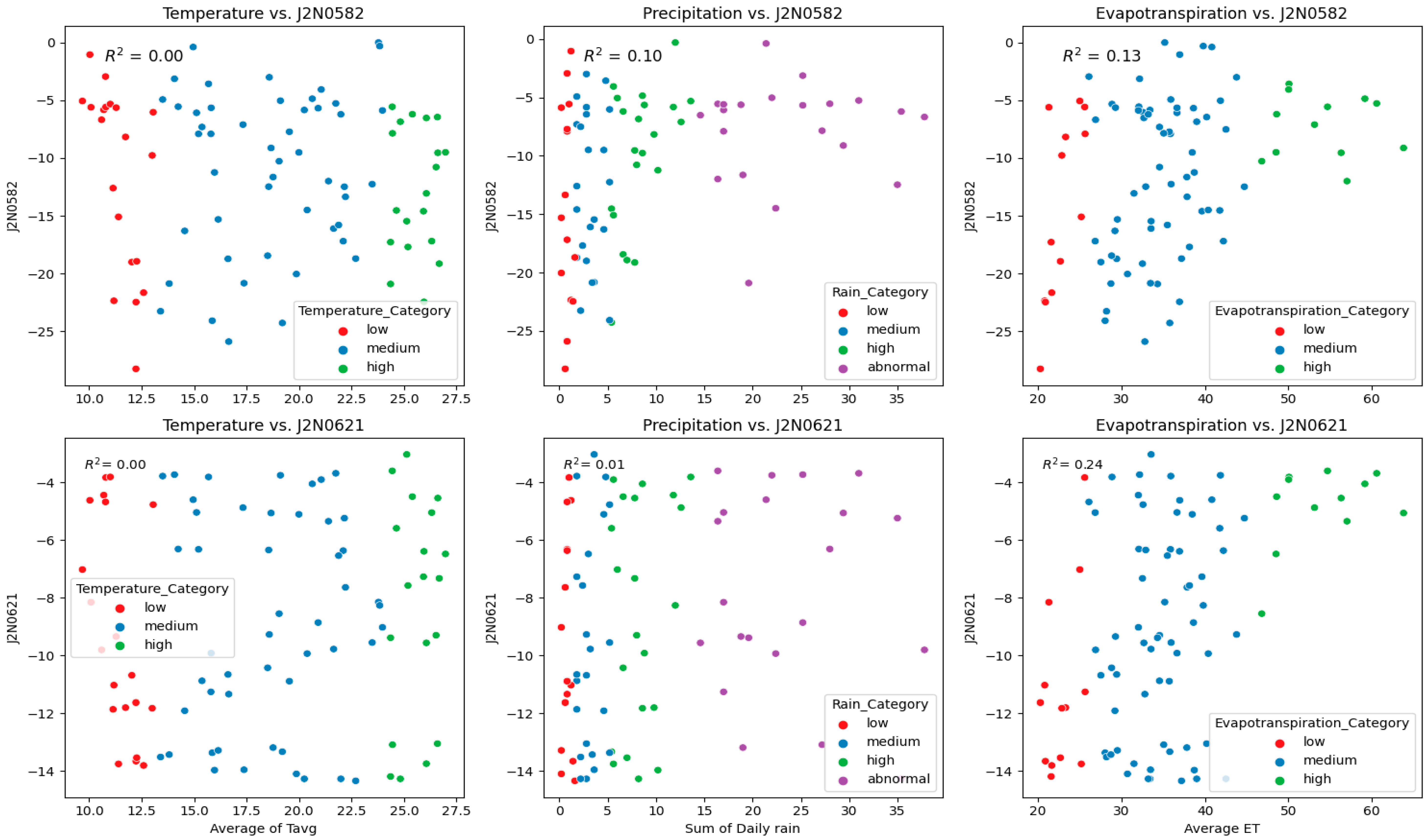
Figure 2.
Scatter plots of the respective independent variables, including average temperature (T, Average of Tavg), summative precipitation (P, Sum of Daily rain), and average evapotranspiration (ET, Average ET) categories for boreholes J2N0582 and J2N0621, the dependent variables. The respective categories of low, medium, high, and abnormal (for P) are color-coded in red, blue, green, and purple, respectively. The individual R2 values are displayed on each graph.
Figure 3.
Scatter plots of the respective independent variables, including average temperature (T, Average of Tavg), summative precipitation (P, Sum of Daily rain), and average evapotranspiration (ET, Average ET) categories for boreholes J2N0019 and J2N0043, the dependent variables. The respective categories of low, medium, high, and abnormal (for P) are color-coded in red, blue, green, and purple, respectively. The individual R2 values are displayed on each graph.
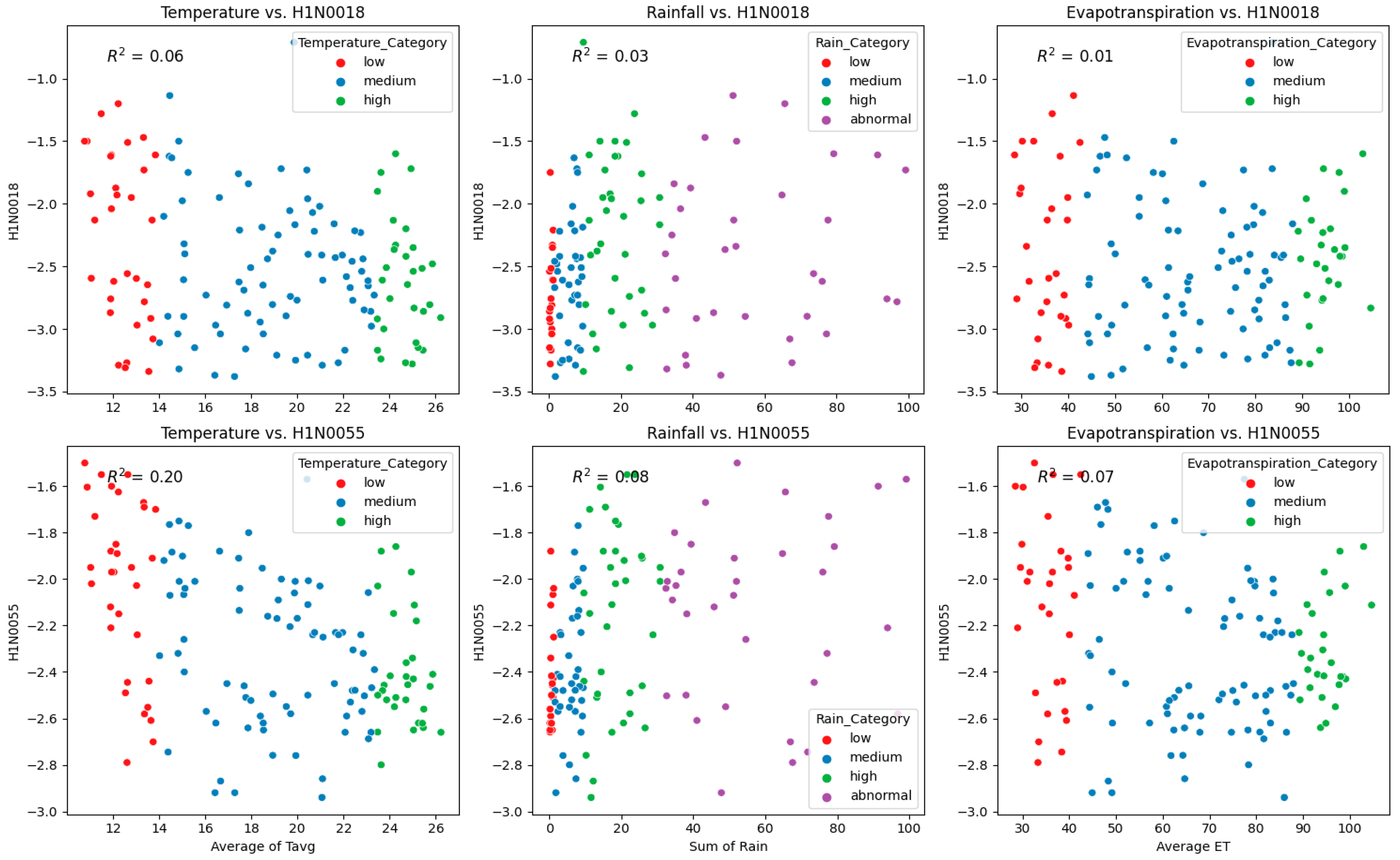
Figure 4.
Scatter plots of the respective independent variables, including average temperature (T, Average of Tavg), summative precipitation (P, Sum of Daily rain), and average evapotranspiration (ET, Average ET) categories for boreholes H1N0018 and H1N0055, the dependent variables. The respective categories of low, medium, high, and abnormal (for P) are color-coded in red, blue, green, and purple, respectively. The individual R2 values are displayed on each graph.
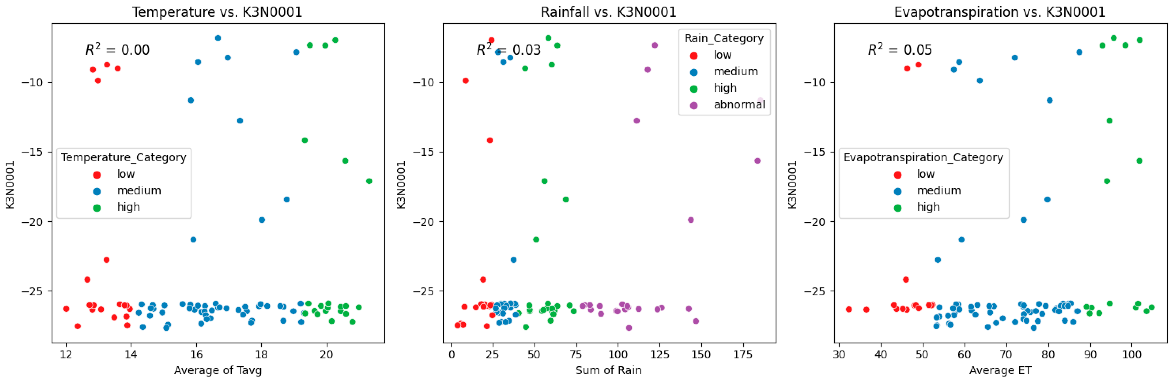
Figure 5.
Scatter plots of the respective independent variables, including average temperature (T, Average of Tavg), summative precipitation (P, Sum of Daily rain), and average evapotranspiration (ET, Average ET) categories for borehole K3N0001, the dependent variables. The respective categories of low, medium, high, and abnormal (for P) are color-coded in red, blue, green, and purple, respectively. The individual R2 values are displayed on each graph.
Table 1.
The chosen boreholes, their respective subregions, the period for which data were available, their location relative to the subregions chosen weather station, and the elevation and status of the borehole.
Table 1.
The chosen boreholes, their respective subregions, the period for which data were available, their location relative to the subregions chosen weather station, and the elevation and status of the borehole.
| Station | Borehole ID | Subregion According to Köppen-Geiger Classification | Period Analyzed | Distance and Direction from the Station | Elevation (m) | Usage Status |
|---|
| Beaufort West | J2N0001 | BWk | 1963–2021 | 10.1 km N | 944 | Local municipal use |
| J2N0019 | 1974–2019 | 1.5 km E | 852 |
| J2N0041 | 1974–2021 | 4.7 km SW | 860 |
| J2N0043 | 2007–2021 | 9.1 km NNW | 1074 |
| J2N0550 | 1975–present | 22.6 km NE | 979 | In use: Unknown consumer |
| J2N0618 | 2004–present | 1 km WNW | 869 |
| George | K3N0001 | Cfb | 2014–2022 | 9.8 km NE | 334 | In use: Unknown consumer |
| Prins Albert | J2N0580 | BWh | 2005–2022 | 13.1 km S | 705 | In use: Unknown consumer |
| J2N0582 | 2005–2022 | 15.5 km S | 762 |
| J2N0620 | 2006–2022 | 15.6 km S | 742 |
| J2N0621 | 2007–2022 | 11.3 km S | 674 |
| Worcester | H1N0018 | Csa | 1981–2022 | 3.8 km SW | 205 | In use: Unknown consumer |
| H1N0055 | 1978–2022 | 1 km SE | 209 |
| H2N0521 | 2004–2022 | 5.2 km NE | 247 |
Table 2.
Categories that were used to separate temperature (T), precipitation (P), and evapotranspiration (ET) into low, medium, and high categories, with the additional category of ‘abnormal’ for extreme P for each of the respective subregions, i.e., BWh, BWk, Csa, and Cfb (N/A = Not applicable).
Table 2.
Categories that were used to separate temperature (T), precipitation (P), and evapotranspiration (ET) into low, medium, and high categories, with the additional category of ‘abnormal’ for extreme P for each of the respective subregions, i.e., BWh, BWk, Csa, and Cfb (N/A = Not applicable).
| Category | T (°C) | P (mm) | ET (mm) |
|---|
| BWh |
| Low (also minimum) | 9.7 | 0 | 19.9 |
| Medium | 13.2 | 1.6 | 25.8 |
| High | 24 | 5.2 | 45.1 |
| Abnormal | N/A | 13.6 | N/A |
| Maximum | 27.1 | 43.8 | 63.8 |
| BWk |
| Low (also minimum) | 9.2 | 0 | 24.2 |
| Medium | 13.8 | 5.5 | 33.7 |
| High | 23.01 | 13 | 56.9 |
| Abnormal | N/A | 25.7 | N/A |
| Maximum | 25.9 | 72.2 | 71 |
| Csa |
| Low (also minimum) | 10.3 | 0 | 28.2 |
| Medium | 14 | 1.2 | 43.6 |
| High | 23.4 | 9.4 | 88.3 |
| Abnormal | N/A | 30.8 | N/A |
| Maximum | 27 | 99.2 | 107.1 |
| Cfb |
| Low (also minimum) | 11.55 | 0 | 32.33 |
| Medium | 14.07 | 26.41 | 53.21 |
| High | 19.33 | 39.75 | 88.53 |
| Abnormal | N/A | 74.93 | N/A |
| Maximum | 21.31 | 185.41 | 104.91 |
Table 3.
Basic descriptive statistics, including the count, mean, standard deviation (std), minimum (min), 25% percentile, 50% percentile, 75% percentile, and maximum (max) of all variables from all four subregions. Climate variables included temperature (T), precipitation (P), and evapotranspiration (ET). Boreholes from each subregion included J2N0580, J2N0582, J2N0620, and J2N0621 in the BWh subregion, J2N0001, J2N0019, J2N0041, J2N0043, J2N0550, and J2N0618 in the BWk subregion, H1N0018, H1N0055, and H2N0521 in the Csa subregion, and lastly, K3N0001 in the Cfb subregion.
| | BWh | BWk | Csa | Cfb |
|---|
| | T | P | ET | J2N0580 | J2N0582 | J2N0620 | J2N0621 | T | P | ET | J2N0001 | J2N0019 | J2N0041 | J2N0043 | J2N0550 | J2N0618 | T | P | ET | H1N0018 | H1N0055 | H2N0521 | T | P | ET | K3N0001 |
|---|
| Units | °C | mm | mm | m | m | m | m | °C | mm | Mm | m | m | m | m | m | m | °C | mm | mm | m | m | m | °C | mm | mm | m |
|---|
| count | 89 | 127 | 141 | 96 |
| mean | 18.6 | 9.0 | 35.4 | −13 | −11.4 | −10.2 | −8.9 | 18.4 | 17.8 | 45.30 | −18.1 | −18.2 | −26.2 | −23.4 | −15.9 | −28.8 | 18.7 | 20.0 | 65.9 | −2.5 | −2.3 | −13.4 | 16.7 | 54.2 | 70.9 | −23.5 |
| std | 5.4 | 10.3 | 9.6 | 6.9 | 6.8 | 1.4 | 3.7 | 4.6 | 16.4 | 11.6 | 19.3 | 10.7 | 12.2 | 12.8 | 3.2 | 7.8 | 4.7 | 24.4 | 22.4 | 0.6 | 0.3 | 1.4 | 2.6 | 41.4 | 17.7 | 6.3 |
| min | 9.7 | 0.0 | 19.6 | −34.3 | −28.2 | −15.8 | −14.3 | 9.2 | 0.0 | 24.2 | −55.7 | −42.0 | −49.1 | −57.4 | −19.5 | −39.2 | 10.3 | 0.0 | 28.2 | −3.4 | −2.9 | −15.9 | 11.6 | 0.0 | 32.3 | −27.7 |
| 25% | 13.8 | 1.6 | 28.9 | −11.1 | −17.2 | −11.1 | −11.9 | 14.6 | 5.5 | 36.4 | −29.8 | −26.2 | −35.1 | −30.6 | −18.6 | −35.4 | 14.4 | 1.2 | 44.9 | −2.9 | −2.5 | −14.9 | 14.5 | 26.4 | 57.1 | −26.6 |
| 50% | 18.8 | 5.2 | 34.6 | −10.5 | −9.5 | −10.3 | −9.3 | 18.3 | 13.0 | 46.8 | −8.1 | −16.1 | −27.8 | −26.5 | −16.9 | −31.5 | 18.9 | 9.4 | 65.6 | −2.6 | −2.3 | −12.8 | 16.5 | 39.8 | 72.8 | −262 |
| 75% | 23.8 | 13.6 | 39.6 | −9.8 | −5.8 | −9.2 | −5.1 | 22.5 | 25.7 | 52.7 | −1.6 | −8.5 | −13.4 | −12.6 | −13.3 | −20.1 | 23.1 | 30.8 | 84.6 | −2.1 | −2.0 | −12.3 | 19.2 | 78.9 | 84.2 | −25.9 |
| max | 27.1 | 43.8 | 63.8 | −6.4 | 0.0 | −7.7 | −3.0 | 25.9 | 72.2 | 71.0 | −0.1 | −0.3 | −6.3 | −4.6 | −9.8 | −15.8 | 26.9 | 99.2 | 107.1 | −0.7 | −1.5 | −11.7 | 21.3 | 185.4 | 104.9 | −6.8 |
Table 4.
Multiple Linear Regression (MLR) test results for each borehole from each subregion with outliers removed. The R2 value indicated the extent to which the model can explain the variance in the dependent variable. The F-statistic and corresponding p-value indicated that all models were statistically significant, except for H2N0521 in the Csa subregion. The least complex models were the lowest relative Akaike Information Criterion (AIC) and Bayesian Information Criteria (BIC) values. The constant indicated the value of the respective dependent variables when all other variables were zero. The statistically significant coefficients (according to their p-values) are highlighted in green. Lastly, the resulting regression equation and the confidence intervals indicate the error range in the final result (N/A = Not applicable).
| | Coefficients | p-Values | |
|---|
| Subregion | Borehole | R2 | F-Statistic | F Stat p-Value | AIC | BIC | Constant | T | P | ET | T | P | ET | Formula | Confidence Intervals |
|---|
| BWh | J2N0580 | 9.6% | 4.5 | 0.01 | 593.1 | 600.6 | −14.4 | −0.4 | N/A | 0.2 | 0.02 | N/A | 0.0 | + ε | [−9.7; −21.7] |
| J2N0582 | 23.8% | 8.9 | 3.6 × 10⁻⁵ | 577.3 | 587.3 | −17.6 | −0.3 | 0.2 | 0.3 | 0.02 | 0.02 | 0.0 | | [−14.6; −25.6] |
| J2N0620 | 17.2% | 8.9 | 0.0003 | 304.6 | 312.1 | −10.5 | −0.1 | N/A | 0.1 | 0.0 | N/A | 0.0 | + ε | [−9.7; −12.1] |
| J2N0621 | 29.2% | 17.8 | 3.4 × 10⁻⁷ | 459.0 | 466.4 | −14.0 | −0.2 | N/A | 0.2 | 0.01 | N/A | 0.0 | + ε | [−12.3; −17.9] |
| BWk | J2N0001 | 18.9% | 14.5 | 2.2 × 10⁻⁶ | 1090.0 | 1098.0 | −15.1 | −2.6 | N/A | 1.0 | 0.0 | N/A | 0.0 | | [−15; −41.8] |
| J2N0019 | 29.9% | 26.5 | 2.7 × 10⁻¹⁰ | 921.2 | 929.7 | −5.5 | −1.9 | N/A | 0.5 | 0.0 | N/A | 0.0 | | [−5.4; −19.2] |
| J2N0041 | 26.2% | 14.6 | 3.5 × 10⁻⁸ | 963.5 | 974.9 | −21.9 | −2.0 | 0.1 | 0.7 | 0.0 | 0.03 | 0.0 | + ε | [−30.5; −32.3] |
| J2N0043 | 12.5% | 8.9 | 0.0003 | 995.9 | 1004.0 | −13.0 | −1.5 | N/A | 0.4 | 0.0 | N/A | 0.01 | | [−8.8; −27.3] |
| J2N0550 | 19.3% | 14.8 | 1.7 × 10⁻⁶ | 632.7 | 641.2 | −16.3 | −0.4 | N/A | 0.2 | 0.0 | N/A | 0.0 | | [−16.4; −20.8] |
| J2N0618 | 23.1% | 12.3 | 4.3 × 10⁻⁷ | 856.9 | 868.2 | −26.8 | −1.2 | 0.1 | 0.4 | 0.0 | 0.01 | 0.0 | + ε | [−27; −37.7] |
| Csa | H1N0018 | 20.6% | 17.9 | 1.3 × 10⁻⁷ | 213.5 | 222.3 | −1.5 | −0.2 | N/A | 0.03 | 0.0 | N/A | 0.0 | | [1.7; −4.2] |
| H1N0055 | 41.7% | 49.3 | 6.8 × 10⁻¹⁷ | 28.3 | 37.2 | −1.3 | −0.1 | N/A | 0.02 | 0.0 | N/A | 0.0 | | [−0.9; −1.3] |
| H2N0521 | 0.7% | 1.0 | 0.3 | 497.2 | 503.1 | −12.9 | −0.03 | N/A | N/A | 0.3 | N/A | N/A | N/A | N/A |
| Cfb | K3N0001 | 9.8% | 5.0 | 0.009 | 620.9 | 628.6 | −21.6 | −0.9 | N/A | 0.2 | 0.03 | N/A | 0.0 | + ε | [−21.1; −23.6] |
Table 5.
Additional information about each borehole’s Multiple Linear Regression (MLR) models. The omnibus and Jarque-Bera values (with their
p-values) indicate the distribution of the residuals. The Durbin-Watson indicates autocorrelation. Skew and kurtosis provide insight into the distribution’s tails and the multicollinearity conditioning number. The standard errors and critical t-value (the critical t-value was derived from a standard t-table using the number of records for each borehole as the degrees of freedom and a 95% confidence interval) were used to calculate the confidence intervals in
Table 4 (N/A = Not applicable).
| | Standard Errors | |
|---|
| Subregion | Borehole | Omnibus (p-Value) | Jarque-Bera (JB) (p-Value) | Durbin-Watson | Skewness | Kurtosis | Conditioning Number | Constant | T | P | ET | Critical t Value |
|---|
| BWh | J2N0580 | 37.7 (0.0) | 64.4 (1.02 × 10⁻¹⁴) | 0.1 | −1.8 | 4.9 | 177 | 3.01 | 0.2 | N/A | 0.09 | 1.99 |
| J2N0582 | 4.8 (0.1) | 6.5 (0.2) | 0.5 | −0.3 | 2.3 | 177 | 2.8 | 0.1 | 0.07 | 0.08 | 1.99 |
| J2N0620 | 66.2 (0.0) | 339.5 (1.92 × 10−74) | 0.6 | −2.3 | 11.1 | 177 | 0.6 | 0.03 | N/A | 0.02 | 1.99 |
| J2N0621 | 1.4 (0.5) | 1.3 (0.5) | 0.5 | 0.1 | 2.5 | 177 | 1.4 | 0.07 | N/A | 0.04 | 1.99 |
| BWk | J2N0001 | 16.3 (0.0) | 16.8 (0.0002) | 0.2 | −0.8 | 2.4 | 223 | 6.7 | 0.5 | N/A | 0.2 | 1.984 |
| J2N0019 | 6.8 (0.01) | 6.7 (0.04) | 0.6 | −0.6 | 3.1 | 220 | 3.5 | 0.3 | N/A | 0.1 | 1.984 |
| J2N0041 | 9.95 (0.01) | 3.9 (0.1) | 0.5 | 0.1 | 2.2 | 240 | 0.3 | 0.3 | 0.06 | 0.1 | 1.984 |
| J2N0043 | 4.8 (0.09) | 4.6 (0.1) | 0.5 | −0.5 | 3.1 | 220 | 4.7 | 0.4 | N/A | 0.1 | 1.984 |
| J2N0550 | 19.1 (0.0) | 9.2 (0.01) | 0.4 | 0.5 | 2.1 | 220 | 1.1 | 0.1 | N/A | 0.03 | 1.984 |
| J2N0618 | 36.2 (0.0) | 8.3 (0.02) | 0.4 | 0.3 | 1.9 | 240 | 2.7 | 0.2 | 0.04 | 0.08 | 1.984 |
| Csa | H1N0018 | 15.9 (0.0) | 29.5 (3.87 × 10⁻⁷) | 0.7 | −0.5 | 4.9 | 327 | 0.2 | 0.03 | N/A | 0.01 | 1.984 |
| H1N0055 | 100.6 (0.0) | 1167.6 (2.85 × 10−254) | 1.1 | −2.2 | 16.1 | 432 | 0.1 | 0.01 | N/A | 0.003 | 1.984 |
| H2N0521 | 42.3 (0.0) | 18.3 (0.0001) | 0.01 | −0.7 | 1.9 | 76.9 | 0.5 | 0.03 | N/A | N/A | N/A |
| Cfb | K3N0001 | 34.9 (0.0) | 55.9 (7.3 × 10⁻¹³) | 0.1 | 1.7 | 4.5 | 115 | 4.2 | 0.4 | N/A | 0.06 | 1.99 |
Table 6.
The Kruskal-Wallis (KW) test results for variable temperature (T), precipitation (P), and evapotranspiration (ET) from each borehole. Larger H statistic values (with p-values < 0.05) render the alternative hypothesis valid, indicating that the medians across the categories differed significantly; the higher the H statistic, the more significant the difference. The highlighted cells indicate statistical significance, according to the p-value.
| | | T | P | ET |
|---|
| | | H Statistic | p-Value | H Statistic | p-Value | H Statistic | p-Value |
|---|
| BWh | J2N0580 | 0.2 | 0.0 | 3.6 | 0.3 | 20.3 | 3.89 × 10⁻⁵ |
| J2N0582 | 1.9 | 0.4 | 2.9 | 0.2 | 6.5 | 0.04 |
| J2N0620 | 2.3 | 0.3 | 7.9 | 0.02 | 6.2 | 0.05 |
| J2N0621 | 0.6 | 0.8 | 0.9 | 0.6 | 19.7 | 5.26 × 10⁻⁵ |
| BWk | J2N0001 | 2.01 | 0.4 | 1.7 | 0.6 | 1.6 | 0.5 |
| J2N0019 | 15.1 | 0.0005 | 1.8 | 0.6 | 1.9 | 0.4 |
| J2N0041 | 4.7 | 0.1 | 0.9 | 0.8 | 1.4 | 0.5 |
| J2N0043 | 7.9 | 0.02 | 1.4 | 0.7 | 0.9 | 0.6 |
| J2N0550 | 1.3 | 0.5 | 1.6 | 0.7 | 4.9 | 0.09 |
| J2N0618 | 2.4 | 0.3 | 3.7 | 0.3 | 2.4 | 0.3 |
| Csa | H1N0018 | 4.9 | 0.1 | 10.5 | 0.02 | 2.09 | 0.4 |
| H1N0055 | 18.3 | 0.0001 | 13.7 | 0.003 | 6.8 | 0.03 |
| H2N0521 | 0.2 | 0.9 | 0.6 | 0.9 | 1.6 | 0.5 |
| Cfb | K3N0001 | 2.4 | 0.3 | 0.1 | 1.0 | 10.6 | 0.01 |
Table 7.
Dunn’s test results for statistically relevant variables from each subregion: temperature (T), precipitation (P), and evapotranspiration (ET). Categories 1, 2, 3, and 4 indicate low, medium, high, and abnormal respectively. Highlighted cells indicate statistically significant categories (N/A = Not applicable).
| | Borehole | Categories | 1 | 2 | 3 | 4 |
|---|
| BWh | ET | J2N0580 | 1 | 1.0 | 0.8 | 0.006 | N/A |
| 2 | 0.8 | 1.0 | 0.0009 | N/A |
| 3 | 0.006 | 0.0009 | 1.0 | N/A |
| P | J2N0582 | 1 | 1.0 | 0.45 | 0.02 | 0.0007 |
| 2 | 0.5 | 1.0 | 0.09 | 0.004 |
| 3 | 0.021 | 0.09 | 1.0 | 0.2 |
| 4 | 0.0007 | 0.004 | 0.2 | 1.0 |
| ET | J2N0582 | 1 | 1.0 | 0.8 | 0.007 | N/A |
| 2 | 0.8 | 1.0 | 0.004 | N/A |
| 3 | 0.007 | 0.004 | 1.0 | N/A |
| P | J2N0620 | 1 | 1.0 | 0.4 | 0.01 | 0.09 |
| 2 | 0.4 | 1.0 | 0.03 | 0.3 |
| 3 | 0.01 | 0.03 | 1.0 | 0.3 |
| 4 | 0.09 | 0.3 | 0.3 | 1.0 |
| ET | J2N0620 | 1 | 1.0 | 0.9 | 0.007 | N/A |
| 2 | 0.9 | 1.0 | 0.003 | N/A |
| 3 | 0.007 | 0.003 | 1.0 | N/A |
| ET | J2N0621 | 1 | 1.0 | 0.43 | 0.002 | N/A |
| 2 | 0.4 | 1.0 | 0.004 | N/A |
| 3 | 0.002 | 0.004 | 1.0 | N/A |
| BWk | T | J2N0019 | 1 | 1.0 | 0.07 | 0.0001 | N/A |
| 2 | 0.07 | 1.0 | 0.01 | N/A |
| 3 | 0.0001 | 0.01 | 1.0 | N/A |
| T | J2N0043 | 1 | 1.0 | 0.2 | 0.01 | N/A |
| 2 | 0.2 | 1.0 | 0.05 | N/A |
| 3 | 0.01 | 0.05 | 1.0 | N/A |
| Csa | P | H1N0018 | 1 | 1.0 | 0.4 | 0.004 | 0.08 |
| 2 | 0.4 | 1.0 | 0.01 | 0.2 |
| 3 | 0.004 | 0.01 | 1.0 | 0.2 |
| 4 | 0.08 | 0.2 | 0.2 | 1.0 |
| T | H1N0055 | 1 | 1.0 | 0.0004 | 0.00006 | N/A |
| 2 | 0.0004 | 1.0 | 0.2 | N/A |
| 3 | 0.00006 | 0.2 | 1.0 | N/A |
| P | H1N0055 | 1 | 1.0 | 0.7 | 0.01 | 0.008 |
| 2 | 0.7 | 1.0 | 0.01 | 0.006 |
| 3 | 0.01 | 0.01 | 1.0 | 0.8 |
| 4 | 0.008 | 0.006 | 0.8 | 1.0 |
| ET | H1N0055 | 1 | 1.0 | 0.01 | 0.09 | N/A |
| 2 | 0.01 | 1.0 | 0.6 | N/A |
| 3 | 0.09 | 0.6 | 1.0 | N/A |
| Cfb | ET | K3N0001 | 1 | 1.0 | 0.05 | 0.5 | N/A |
| 2 | 0.05 | 1.0 | 0.004 | N/A |
| 3 | 0.5 | 0.004 | 1.0 | N/A |


 ,
, 


