Hydrogeochemical Characterization and Determination of Arsenic Sources in the Groundwater of the Alluvial Plain of the Lower Sakarya River Basin, Turkey

Abstract

Arsenic (As) contamination in groundwater represents a major global public health threat, particularly in alluvial aquifer systems where redox-sensitive geochemical processes facilitate the mobilization of naturally occurring trace elements. This study investigates groundwater quality, particularly focusing on the origin of arsenic contamination in shallow and deep alluvial aquifers of the Lower Sakarya River Basin, which are crucial for drinking, domestic, and agricultural uses. Groundwater samples were collected from 34 wells—7 tapping the shallow aquifer (<60 m) and 27 tapping the deep aquifer (>60 m)—during wet and dry seasons for the hydrogeochemical characterization of groundwater. Environmental isotope analysis (δ¹⁸O, δ²H, ³H) was conducted to characterize origin and groundwater residence times, and the possible hydraulic connection between shallow and deep alluvial aquifers. Mineralogical and geochemical characterization of the sediment core samples were carried out using X-ray diffraction and acid digestion analyses to identify mineralogical sources of As and other metals. Pearson correlation coefficient analyses were also applied to the results of the chemical analyses to determine the origin of metal enrichments observed in the groundwater, as well as related geochemical processes. The results reveal that 33–41% of deep groundwater samples contain arsenic concentrations exceeding the WHO and Turkish drinking water standard of 10 µg/L, with maximum values reaching 373 µg/L. Manganese concentrations exceeded the 50 µg/L limit in up to 44% of deep aquifer samples, reaching 1230 µg/L. On the other hand, iron concentrations were consistently low, remaining below the detection limit in nearly all samples. The co-occurrence of As and Mn above their maximum contaminant levels was observed in 30–33% of the wells, exhibiting extremely low sulfate concentrations (0.2–2 mg/L), notably low dissolved oxygen concentration (1.45–3.3 mg/L) alongside high bicarbonate concentrations (450–1429 mg/L), indicating localized varying reducing conditions in the deep alluvial aquifer. The correlations between molybdenum and As (rdry = 0.46, rwet = 0.64) also indicate reducing conditions, where Mo typically mobilizes with As. Arsenic concentrations also showed significant correlations with bicarbonate (HCO₃⁻) (rdry = 0.66, rwet = 0.80), indicating that alkaline or reducing conditions are promoting arsenic mobilization from aquifer materials. All these correlations between elements indicate that coexistence of As with Mn above their MCLs in deep alluvial aquifer groundwater result from reductive dissolution of Mn/Fe(?) oxides, which are primary arsenic hosts, thereby releasing arsenic into groundwater under reducing conditions. In contrast, the shallow aquifer system—although affected by elevated nitrate, sulfate, and chloride levels from agricultural and domestic sources—exhibited consistently low arsenic concentrations below the maximum contaminant level. Seasonal redox fluctuations in the shallow zone influence manganese concentrations, but the aquifer’s more dynamic recharge regime and oxic conditions suppress widespread As mobilization. Mineralogical analysis identified that serpentinite, schist, and other ophiolitic/metamorphic detritus transported by river processes into basin sediments were identified as the main natural sources of arsenic and manganese in groundwater of deep alluvium aquifer.

1. Introduction

Arsenic occurrence in groundwater is a critical concern for public health, affecting millions of people worldwide [1]. Recent global assessments estimate that between 94 and 220 million people across more than 100 countries are exposed to arsenic-contaminated groundwater exceeding the WHO guideline of 10 μg/L [2]. Arsenic is a known carcinogen, and prolonged exposure to arsenic-contaminated drinking water can cause severe health issues such as black foot diseases, skin lesions, cancer, respiratory diseases and cardiovascular disorders [3].

Arsenic is a naturally occurring metalloid which is found in the Earth’s crust at an average concentration of 1.5 mg/kg and forms the chemical constituent of about 245 minerals (e.g., sulfides and ironoxides-oxyhydroxides at high concentrations) at a large range of concentration (0.1–276,000 mg/kg) [4,5]. Arsenic enters groundwater through natural processes such as the weathering of arsenic-bearing minerals in soils and rocks, reductive dissolution, desorption, and geothermal processes, as well as anthropogenic activities including sulfide mining, the application of pesticides in agriculture, industrial operations, and coal combustion. Geogenic origin is the most common cause of arsenic contamination in groundwater globally [6]. The release of arsenic into groundwater depends on arsenic species and geochemical conditions in the aquifer such as pH, redox potential, the presence of competing ions (HCO₃⁻, PO₄⁻³) in the groundwater, mineral phases (especially Fe, Mn, and Al oxyhydroxides), and the organic matter content of the geological media [1,7].

The largest and most serious natural arsenic contamination globally is observed in alluvial aquifers along major rivers and large deltas of south and southeast Asia where millions of people rely heavily on arsenic-contaminated groundwater for drinking and irrigation purposes [1,8,9,10,11,12,13]. Arsenic contamination in groundwater was also reported in many coastal and alluvial aquifers of Turkey and noted to be associated with generally geogenic or geothermal origins [14,15,16,17,18,19,20].

Over the past two decades, integrated field and laboratory approaches have been widely applied to delineate the extent and origin of arsenic contamination in alluvial aquifers. Multivariate statistical techniques such as Pearson correlation, principal component analysis (PCA), and hierarchical cluster analysis (HCA) are commonly used to evaluate associations between trace elements and geochemical parameters, and to infer the dominant hydrochemical processes [10,21]. Mineralogical and geochemical characterization of the aquifer materials along with X-ray diffraction (XRD) and acid digestion followed by ICP-MS analysis are essential for identifying arsenic-bearing phases such as Fe and Mn oxides, clays, and sulfides within aquifer sediments [11]. These methods, when applied in combination, offer a robust framework for understanding arsenic mobilization mechanism in the subsurface environment. Understanding the origin of arsenic contamination in groundwater is crucial for implementing effective mitigation measures, ensuring sustainable resource management and protecting public health.

The main objective of this study is to identify the potential sources and mechanisms responsible for arsenic mobilization in the groundwater of the alluvial plain of the Lower Sakarya River Basin, Turkey. The study employs a combination of geochemical characterization of groundwater and alluvial sediments, mineralogical characterization of the sediment cores, and statistical correlation analyses results to determine the origin of metal enrichments observed in the groundwater, as well as related geochemical processes.

2. Study Area

The study area is located at the lower Sakarya sub-basin of the Sakarya River Basin in northwestern Turkey. The lower Sakarya alluvial plain, also called Adapazarı Basin, is an attractive industrial investment hub; 72% of the alluvial plain is used for agricultural purposes, 9.5% for urban settlement area, 13% for forestry, 4% of it covers industrial zones at the east and west sides of the Sakarya alluvial plain. The lower Sakarya alluvial plain is a fault-bounded plain with a topographic gradient of about 0.6–0.8% to the north, and it occupies an area of nearly 665 km². Based on the long-term meteorological data, the mean annual temperature at the study area is 14 °C, while the mean annual precipitation and actual evapotranspiration are 855 mm and 550 mm, respectively.

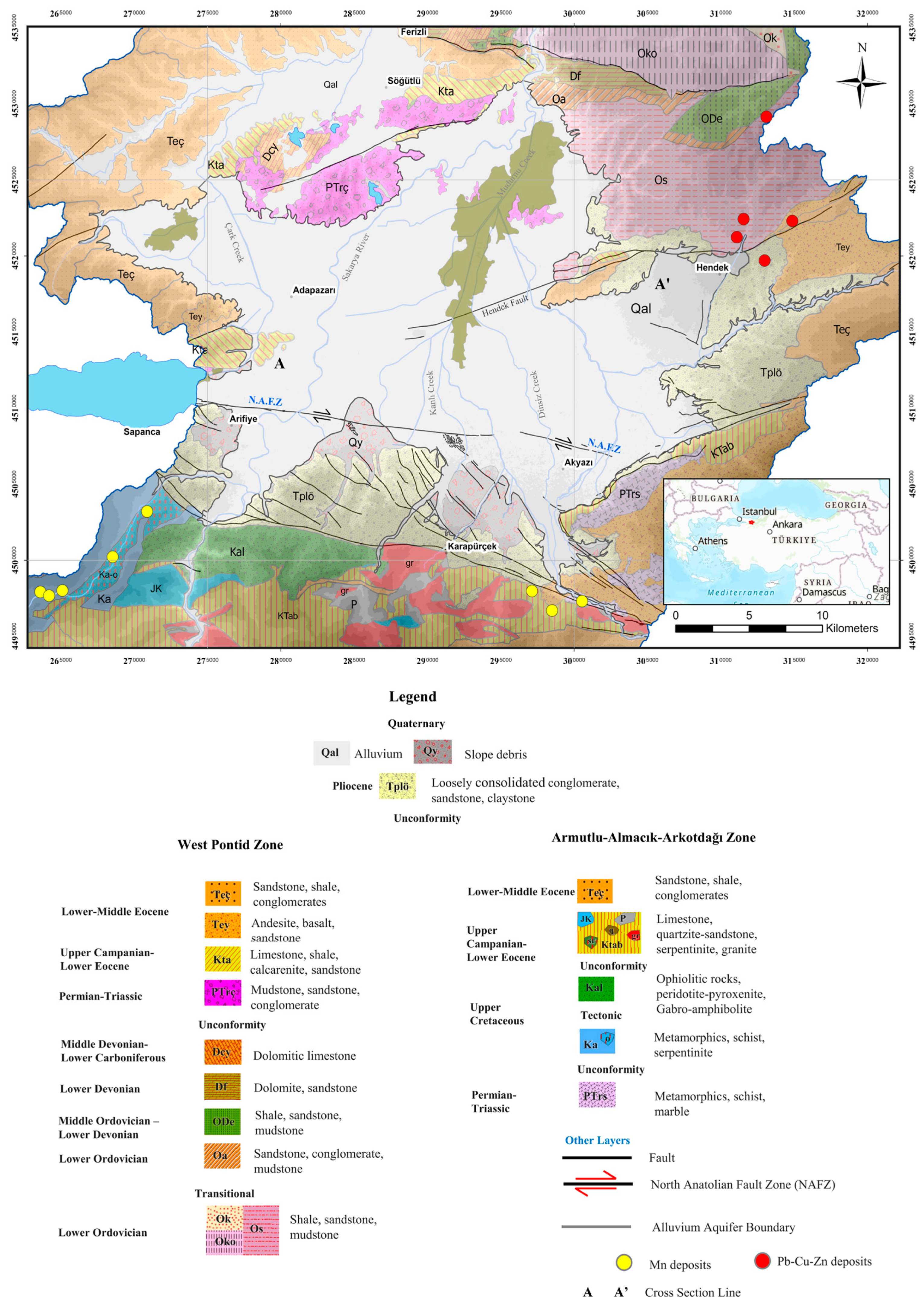
3. Geological Settings

Two distinct tectonic zones and cover units have been identified from north to south within the study area and its vicinity. The Western Pontide zone, comprising the northern half of the lower Sakarya sub-basin, is predominantly characterized by sedimentary rocks dating from the Ordovician to the Eocene period. The Armutlu-Almacık-Arkotdağı zone comprises metamorphic successions and ophiolitic mélange situated between the two principal branches of the North Anatolian Fault (Figure 1) [22,23]. The investigation area comprises Quaternary alluvial deposits that form the Adapazarı, Akyazı, and Hendek plains. These deposits consist of unconsolidated pebbles, sand, silt, and clay, primarily derived from the sediment load of the Sakarya River and its tributaries (Figure 1).

The thickness of the alluvium increases from the basin margins toward the center, reaching a maximum of approximately 350 m in the Lower Sakarya Basin [24]. In the northern part of the plain, the alluvium is about 80–85 m thick, while in the southern region, it may reach 200–250 m. These alluvial deposits overlie and are bounded by bedrock units ranging in age from the Paleozoic to the Cenozoic. Paleozoic formations include shale, sandstone, mudstone, calc-schist, graphite schist, and crystallized limestone. Mesozoic rocks are represented by ultrabasic complexes such as serpentinite. The Tertiary sequence includes andesite, basalt, limestone, and sandstone, whereas the Quaternary deposits are composed of Pliocene-aged conglomerate, sandstone, claystone, and slope debris.

In the southeast and southwest of the Sakarya alluvial plain, metallic deposits such as manganese, iron, and chromium were discovered by the General Directorate of Mineral Research and Exploration (MTA) in the undifferentiated metamorphics and serpentinites (Figure 1) [25]. The ultrabasic complex (serpentinite), containing enclaves of unsegregated phyllite and limestone, exhibits manganese mineralization. The Alaçam Dere Formation is characterized by iron oxide alteration, with the primary ore being sedimentary in origin. Pyrolusite and psilomelane are formed through metamorphic and secondary processes [26]. Similar processes are also observed in other manganese deposits. Manganese mineralization at Tahtacıkerliği Tepe and Alaçam Dere is influenced by the high silica content in phyllites, with quartz as the main gangue mineral. The dominant manganese minerals are pyrolusite (MnO₂) and psilomelane ((Ba,H₂O)₂Mn₅O₁₀), while rhodonite (MnSiO₃) and rhodochrosite (MnCO₃) are present in smaller amounts [26]. This mineralization is consistent with regional lithology and likely represents a potential geogenic source for manganese and associated trace elements observed in the groundwater system, which contains grain particles of varying sizes derived from basement rocks.

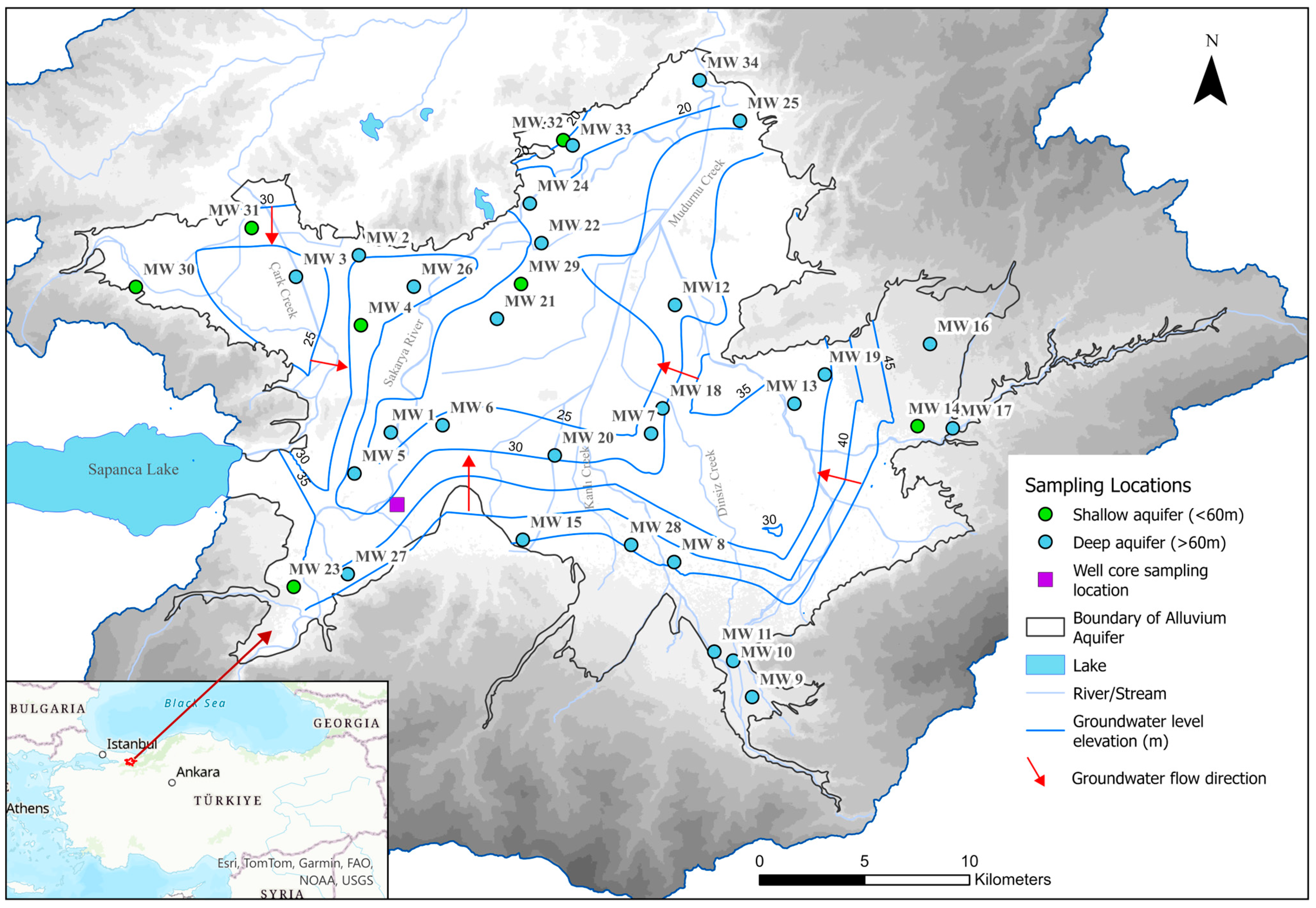
4. Hydrology and Hydrogeology

The Sakarya River serves as the principal watercourse where all tributaries in the lower Sakarya plain converge, flowing northward across the center of the plain with a gradient of 0.5%. It merges with the Mudurnu Stream from the northern section of the plain to the east and with Çarksuyu on the western side, which expels the surplus water from Sapanca Lake (Figure 1).

To delineate the underlying geology and characterize the aquifers, 46 drilling logs compiled by the General Directorate of State Hydraulic Works (DSI) on the alluvial plain have been evaluated. Alluvial aquifer systems comprise two distinct layers (Figure 2). The initial shallow aquifer system is situated within the first 60 m, whereas the subsequent aquifer system may extend from 60 m to a depth of 200 m.

Aquifer strata are confined, exhibiting varied thicknesses of interbedded clay layers in green, blue, and dark grey, interspersed with silt and sand intercalations. Figure 2 illustrates the cross-section of the subsurface geology of the alluvium from west to east.

The shallow aquifer system, exhibiting a varying thickness of 5 to 50 m, possesses unconfined or semi-confined characteristics and is composed of sand, gravel, clay, or their alternations. The second-deep aquifer unit displays confined or semi-confined characteristics and has a thickness ranging from 3 to 90 m. It consists of gravel or sandy gravel derived from several sources, including quartz, marble, serpentine, green schists, opal, mica schists, and peridotite [24].

The primary source of groundwater in the lower Sakarya alluvial plain is the high-yield deep aquifer between the depths of 60 and 180 m. Based on borehole logs that have been received by DSI in 2019, the alluvial aquifer in the plain has specific well capacities that range from 0.50 to 50 L per second per meter (l/s/m).

The highest specific well capacities in the plain were observed in Akyazı, ranging from 40 to 42 l/s/m, and in Arifiye—located in close proximity to the Sakarya River—varying between 10 and 20 l/s/m. The hydraulic conductivities of alluvium in the deeper aquifer range from 3.09 × 10⁻⁴ to 4.55 × 10⁻⁴ m/s [24]. The groundwater level in the wells is within depths of 0–7 m below ground surface in the central and northern part of the alluvium plain; the depth to groundwater increases to 10–15 m in the southern boundary as a result of continuous pumping from organized industrial sites and local establishments such as greenhouses and cement factories, as indicated by water level measurements. The main direction of groundwater flow in the alluvial plain is located towards the Sakarya River and ultimately to the north of the basin (Figure 3).

5. Materials and Methods

In order to determine the hydrogeochemical properties of the shallow and deep aquifer systems, the groundwater monitoring stations were categorized into two distinct groups. Seven stations represented the shallow aquifer system, whereas twenty-seven stations represented the deep aquifer system. The sampling locations were chosen based on land use classification, groundwater flow direction, and aquifer type and depth.

Groundwater sampling surveys were conducted between September 2018 and April 2019 representing both dry and wet periods. Groundwater samples (n = 34) were obtained from wells utilized for domestic, agricultural, or industrial purposes. In field studies, the electrical conductivity (EC), pH, dissolved oxygen (DO) concentration and temperature (T) of water samples were measured in situ using a multi-parameter measuring instrument (Thermo Orion 5 Star, Waltham, MA, USA). The samples were filtered via a 0.45 μm cellulose acetate syringe filter and subsequently placed into plastic bottles. Water samples taken for elemental analysis were acidified to a pH of less than 2 using supra pure nitric acid. Additional samples were collected without preservation and maintained at 4 °C in the refrigerator until analysis.

The concentrations of major and trace elements (Ca, Mg, Na, K, Al, As, Ba, Cr, Cd, Cu, Co, Fe, Mn, Mo, Ni, Pb, Se, Sb, Sn, U, V, Zn) were analyzed using a Perkin Elmer Elan DRC-e model ICP-MS (Inductively Coupled Plasma Mass Spectrometer, Waltham, MA, USA) in Kocaeli University Environmental Hydrogeochemistry and Hydrogeology Laboratory. An internal standard mix (20 ppb Re and Rh) was added to each sample online to eliminate the analytical errors resulting from the sample matrix. The concentrations of major anions (Cl⁻, SO₄²⁻, NO₃⁻, F⁻) in the samples were quantified using ion chromatography (Dionex IC-1100, Waltham, MA, USA). The concentration of HCO₃⁻ was ascertained using the acid titration method [27]. The Charge Balance Error (CBE) in the majority of water samples was below 10%, ranging from an average of 2.5% during the dry period to 7.26% during wet period analyses. A high Charge Balance Error (CBE) was observed only in a few wet season samples, likely due to significant contamination associated with unmeasured analytes. Relative measurement uncertainty values lay between 1 and 12% for ICP-MS, 4% and 7% for ion chromatography.

To assess the residence time of groundwater in aquifers and the extent of connectivity between deep and shallow aquifers, environmental isotope concentrations of oxygen-18 (δ¹⁸O), deuterium (δ²H), and tritium (³H) were measured from samples collected during both wet and dry periods; the analyses were conducted at the State Hydraulic Works (DSİ) Isotope Laboratory under the Technical Research and Quality Control Department in Ankara, Turkey. All measurements were performed using internationally accepted IAEA standard methods (optical spectroscopy for δ¹⁸O and δ²H; electrolytic enrichment and liquid scintillation counting for ³H). The isotope ratios for δ¹⁸O and δ²H were expressed in per mil (‰) relative to the Vienna Standard Mean Ocean Water (VSMOW), which is the global reference standard for stable isotope ratios in water. To ensure data quality and traceability, all analyses were performed under the laboratory’s internal QA/QC protocols including the use of certified reference materials, regular calibration against VSMOW standards, and the inclusion of laboratory blanks. The measurement uncertainty was reported for each individual sample: typically, ±0.10–0.15‰ for δ¹⁸O, ±0.9–1.1‰ for δ²H, and ±0.55–0.95 TU for tritium analyses.

Borehole sediment core samples were collected at various depths in the Alancuma and Akyazı districts (Figure 3), where anomalies of arsenic (As) and manganese (Mn) were detected. To ascertain their sources in the alluvial aquifer, their concentration levels in the sediments were examined, and the mineral phases correlated with elevated As and Mn concentrations.

Sediment samples were air-dried and subsequently pulverized into a fine powder using a pulveriser. Subsequently, 1 g of the powdered material was digested in 10 mL of supra-pure HNO₃ at 90 °C on a hot plate for a duration of 2 h. Subsequently, 1 mL of the digested sample was diluted in a 1:10 ratio with ultrapure water before ICP-MS analysis.

The sediment samples were characterized mineralogically by X-ray diffraction (XRD, Bruker D8 advance model, Billerica, MA, USA) investigations. XRD measurements were performed on powder samples derived from dehumidified materials, ground to less than 75 μm, and arranged in the sample cup to ensure random particle orientation. These measurements were conducted in the XRD Laboratory of the Istanbul Technical University (ITU) Geology Department using a device operating at 40 mA and 40 kV, employing unfiltered Cu Kα radiation, with a step speed of 2° 2 θ/min over a range of 0–72° 2 θ, utilizing a specialized Lynxeye detector (Billerica, MA, USA). The X-ray data were analyzed utilizing the “PDF-2” database and the “Jade 6.5” data assessment software (Materials Data, Inc., n.d., Livermore, CA, USA).

Pearson correlation tests (p < 0.01, 0.05) were conducted on the results using IBM SPSS Statistics20 software to determine the sources of contamination and the interrelationships among chemical parameters. Two-tailed significance values were employed for the correlation analysis.

To ascertain the direction of groundwater flow within the deep alluvial aquifer system of the Adapazarı (located in the Söğütlü-Ferizli Plain), Akyazı-Karapürçek, and Hendek Plains of the Lower Sakarya Basin, static water level measurements were conducted at 41 well sites, encompassing both dry and wet periods during 2018–2019.

6. Results and Discussion

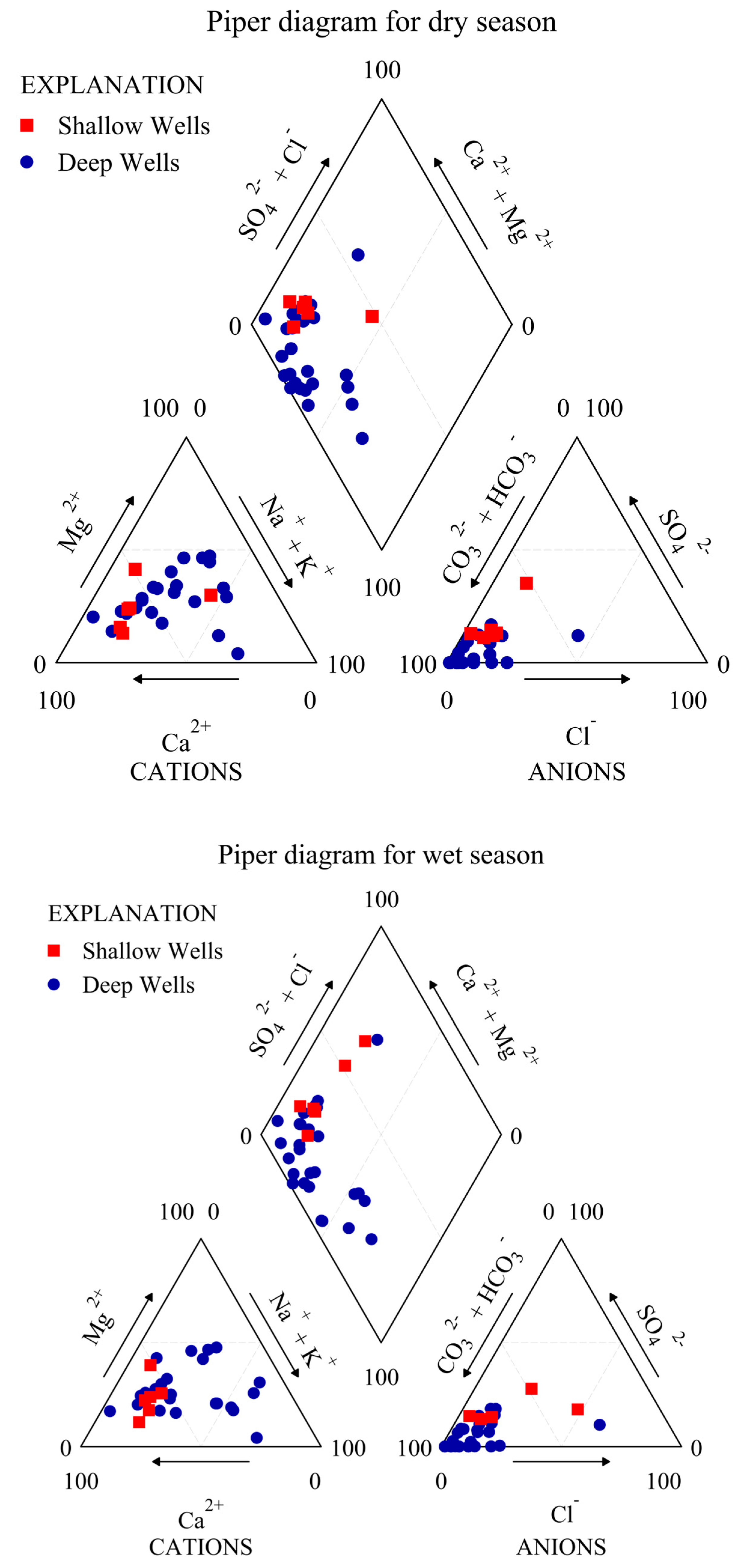
6.1. Assessment of Hydrogeochemical Characteristics and Groundwater Quality of Alluvium Aquifer

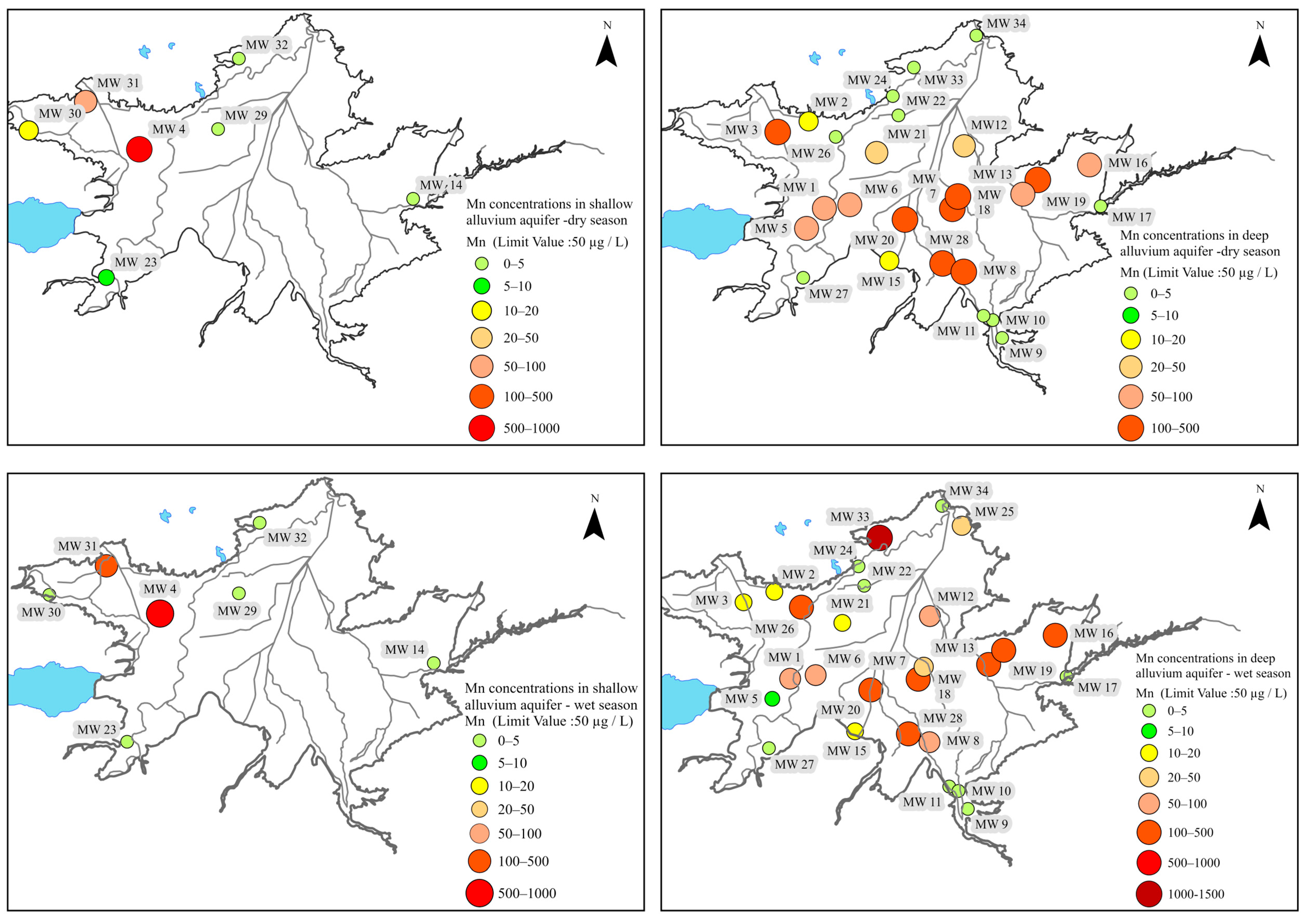
6.1.1. Shallow Alluvium Aquifer

Groundwater in the shallow alluvial aquifer exhibits a neutral to alkaline character with a mean pH value of 7.66 ± 0.49 (stdev). The electrical conductivity values vary from 173 to 3290 µS/cm (986.4 µS/cm ± 855.6). Groundwater with high EC values shows enrichment either in chloride, sulfate or both compared to groundwater exhibiting a low EC (

Table A1. Physicochemical properties of groundwater collected from the shallow aquifer for the dry season in the Lower Sakarya Plain (September 2018).

Sample No	pH	DO	EC	Na+	K+	Ca2+	Mg2+	Cl−	SO42−	HCO3−	F−	NO3−
		mg/L	µS/cm at 25 °C	mg/L	mg/L	mg/L	mg/L	mg/L	mg/L	mg/l	mg/L	mg/L
MW 4	7.17	1.29	1590.40	48.71	19.24	104.38	46.59	30.76	81.32	456.21	0.37	0.11
MW 14	8.20	10.43	173.74	5.81	0.16	20.80	2.95	1.39	9.17	73.86	<0.15	2.20
MW 23	7.30	7.68	924.00	17.48	2.98	85.01	43.67	25.05	44.13	401.55	0.18	10.17
MW 29	8.09	10.39	246.40	8.63	1.37	31.67	7.56	10.95	15.70	110.63	0.15	0.31
MW 30	7.89	5.02	772.70	26.91	1.80	86.83	10.16	22.00	44.50	294.29	0.16	15.01
MW 31	7.22	4.67	2258.00	189.28	0.31	94.89	67.41	73.09	270.10	503.63	1.01	77.40
MW 32	7.16	1.40	460.00	9.02	1.44	31.69	7.86	10.44	14.90	116.46	0.12	0.41
Min	7.16	1.29	173.74	5.81	0.16	20.80	2.95	1.39	9.17	73.86	0.12	0.11
Max	8.20	10.43	2258.00	189.28	19.24	104.38	67.41	73.09	270.10	503.63	1.01	77.43
Mean	7.58	7.13	917.89	43.69	3.90	65.04	26.60	24.81	68.55	279.52	0.33	15.09
STDV	0.43	3.32	705.45	61.01	6.32	32.72	23.60	21.78	85.49	166.46	0.31	26.02

and

Table A2. Physicochemical properties of groundwater collected from the shallow aquifer for the wet season in the Lower Sakarya Plain (April 2019).

Sample No	pH	DO	EC	Na+	K+	Ca2+	Mg2+	Cl−	SO42−	HCO3−	F−	NO3−
		mg/L	µS/cm at 25 °C	mg/L	mg/L	mg/L	mg/L	mg/L	mg/L	mg/l	mg/L	mg/L
MW 4	7.21	2.56	1285.20	33.53	15.75	107.79	33.32	43.61	59.65	559.80	0.34	0.56
MW 14	8.36	11.58	227.36	4.93	0.13	13.96	2.35	2.49	11.26	76.80	0.13	3.42
MW 23	7.57	2.86	952.00	14.16	2.38	74.14	34.17	29.20	53.62	393.57	0.10	11.34
MW 29	8.03	9.08	435.30	6.94	1.27	26.76	5.80	13.51	18.75	118.89	0.18	83.93
MW 30	8.15	10.71	323.12	7.06	1.26	23.67	5.76	13.59	18.78	119.09	0.20	1.01
MW 31	6.78	4.44	3290.22	106.79	12.79	256.71	74.32	580.84	294.12	714.00	0.74	196.71
MW 32	8.05	1.88	871.60	28.50	1.19	96.78	9.85	46.36	73.85	161.42	0.25	32.53
Min	6.78	1.88	227.36	4.93	0.13	13.96	2.35	2.49	11.26	76.80	0.10	0.56
Max	8.36	11.58	3290.22	106.79	15.75	256.71	74.32	580.84	294.12	714.00	0.74	196.71
Mean	7.74	6.16	1054.97	28.84	4.97	85.69	23.65	104.23	75.72	306.22	0.28	47.07
STDV	0.53	3.85	978.20	33.46	5.97	77.88	24.07	195.16	91.88	233.58	0.20	67.00

). The mean dissolved oxygen (DO) concentration of shallow aquifer groundwater was 7.13 ± 3.32 mg/L and 6.16 ± 3.85 mg/L at dry and wet periods, respectively. While oxic conditions were generally dominant throughout the aquifer, a few groundwater samples—specifically MW-4 and MW-32—showed persistently low dissolved oxygen (DO) levels (ranging from 1.29 to 2.56 mg/L) in both sampling periods. This suggests that suboxic conditions may also be present in certain zones, likely influenced by localized variations in redox dynamics or organic matter availability.

Except for a single well (MW-31), which exhibited markedly elevated sodium concentrations (106.79–189.28 mg/L), calcium was the predominant cation in the shallow groundwater, with average concentrations ranging between 65.04 and 85.69 mg/L. Seasonal variation was observed in water facies of shallow groundwater from Ca-Mg-HCO₃, Ca-HCO₃, Na-Mg-Ca-HCO₃-SO₄ in dry period to Ca-Mg-HCO₃, Ca-Mg-Cl-HCO₃-SO₄, Ca-Mg-HCO₃-NO₃, Ca-HCO₃-SO₄-Cl in wet period (Figure 4). As discussed later in Section 6.2, the widespread presence of calcite in the alluvium accounts for the dominance of calcium–bicarbonate water types in groundwater. Shifts in the order of dominant anions—particularly Cl⁻, NO₃⁻, and SO₄²⁻—observed in some wet season samples also indicate potential signs of anthropogenic contamination.

Arsenic concentrations in shallow aquifer groundwater samples remained below permissible limit value of 10 µg/L with a mean concentration varying from 3.95 µg/L ± 1.62 (stdev) in dry periods to 2.69 µg/L ± 3.09 (stdev) in wet periods (

Table A3. Descriptive statistics of trace element contents of groundwater samples collected from the shallow aquifer in the Lower Sakarya Plain for the dry season (September 2018).

Sample No	Al	As	Ba	Cd	Co	Cr	Cu	Fe	Mn	Mo	Ni	Pb	Sb	Se	Sn	U	V	Zn
	µg/L	µg/L	µg/L	µg/L	µg/L	µg/L	µg/L	µg/L	µg/L	µg/L	µg/L	µg/L	µg/L	µg/L	µg/L	µg/L	µg/L	µg/L
MW 4	5.84	1.08	238.56	<0.01	0.49	4.71	0.11	<5	783.27	4.37	9.91	<0.01	0.10	0.44	<0.01	3.20	1.20	3.28
MW 14	2.23	0.54	19.97	<0.01	0.04	1.21	<0.1	<5	0.05	0.38	0.84	0.09	0.09	0.30	<0.01	0.11	5.38	18.51
MW 23	6.95	0.84	29.46	<0.01	0.27	2.63	2.32	<5	5.50	0.29	23.69	0.17	0.49	1.08	<0.01	0.35	1.01	73.26
MW 29	11.40	3.80	8.47	0.05	0.12	0.53	0.45	<5	1.53	0.30	3.03	0.66	0.31	0.55	<0.01	0.42	0.05	6.27
MW 30	2.87	0.30	36.91	0.04	0.43	1.94	1.73	<5	11.23	0.20	5.62	0.23	0.46	0.80	0.10	0.89	0.08	441.58
MW 31	5.55	0.84	40.05	<0.01	0.25	1.81	1.20	<5	51.14	0.26	5.76	0.04	0.25	2.53	0.07	7.18	1.51	6.66
MW 32	9.20	3.95	9.29	0.11	0.09	1.21	9.69	<5	0.22	0.31	56.88	0.76	0.35	0.48	1.30	0.37	0.09	153.69
Min	2.23	0.30	8.47	<0.01	0.04	0.53	<0.1	<5	0.05	0.20	0.84	<0.01	0.09	0.30	<0.01	0.11	0.05	3.28
Max	11.40	3.95	238.56	0.11	0.49	4.71	9.69	<5	783.27	4.37	56.88	0.76	0.49	2.53	1.30	7.18	5.38	441.58
Mean	6.29	1.62	54.67	0.07	0.24	2.01	2.58	-	121.85	0.87	15.10	0.33	0.29	0.88	0.49	1.79	1.33	100.47
STDV	3.02	1.44	75.95	0.03	0.16	1.27	3.26	-	270.54	1.43	18.41	0.28	0.15	0.72	0.57	2.41	1.74	148.21

and

Table A4. Descriptive statistics of trace element contents of groundwater samples collected from the shallow aquifer in the Lower Sakarya Plain for the wet season (April 2019).

Sample No	Al	As	Ba	Cd	Co	Cr	Cu	Fe	Mn	Mo	Ni	Pb	Sb	Se	Sn	U	V	Zn
	µg/L	µg/L	µg/L	µg/L	µg/L	µg/L	µg/L	µg/L	µg/L	µg/L	µg/L	µg/L	µg/L	µg/L	µg/L	µg/L	µg/L	µg/L
MW 4	<0.1	1.03	218.31	0.05	0.54	2.69	1.66	<1	588.59	3.03	9.97	0.05	0.72	0.21	0.40	2.76	1.06	19.95
MW 14	<0.1	0.53	18.18	<0.001	0.05	1.81	0.40	<1	0.01	0.35	1.90	0.04	0.75	0.19	0.02	0.09	4.74	8.83
MW 23	<0.1	0.91	26.58	0.01	0.24	7.17	0.96	<1	1.81	0.22	25.26	<0.01	0.85	0.98	0.16	0.27	1.40	132.18
MW 29	19.27	2.90	9.85	0.51	0.28	2.20	1.10	<1	0.46	0.27	2.90	7.06	0.52	0.48	0.11	0.32	0.18	13.70
MW 30	43.81	3.16	7.48	0.01	0.09	2.02	1.14	<1	0.14	0.29	2.71	0.03	0.85	0.71	0.05	0.41	0.18	4.03
MW 31	0.88	9.83	110.14	0.16	1.10	23.65	4.07	<1	471.03	0.71	28.66	0.02	0.85	4.23	0.18	16.14	7.58	24.08
MW 32	<0.1	0.47	46.94	0.01	0.30	2.06	0.33	<1	0.97	0.11	8.12	<0.01	0.43	1.04	0.03	0.96	0.86	64.56
Min	<0.1	0.47	7.48	<0.001	0.05	1.81	0.33	<1	0.01	0.11	1.90	<0.01	0.43	0.19	0.02	0.09	0.18	4.03
Max	43.81	9.83	218.31	0.51	1.10	23.65	4.07	<1	588.59	3.03	28.66	7.06	0.85	4.23	0.40	16.14	7.58	132.18
Mean	21.32	2.69	62.50	0.12	0.37	5.94	1.38	-	151.86	0.71	11.36	1.44	0.71	1.12	0.13	2.99	2.29	38.19
STDV	17.59	3.09	71.56	0.18	0.33	7.44	1.18	-	241.09	0.96	10.29	2.81	0.16	1.31	0.12	5.44	2.60	42.58

).

Manganese and nickel concentrations exceeded their respective maximum contaminant levels (MCLs) in some groundwater samples collected during both the dry and wet seasons. Overall, 28% of the samples from the shallow alluvial aquifer system exhibited manganese concentrations above the MCL of 50 µg/L. In well MW4, manganese levels reached 783.27 µg/L during the dry season and decreased to 588.59 µg/L in the wet season. Conversely, MW31 showed an increase in manganese from 51.14 µg/L in the dry period to 471.03 µg/L in the wet period (Table A3 and Table A4). Nickel concentrations above the MCL of 20 µg/L were also observed in three of the seven groundwater samples (MW23, MW31, and MW32). In wells MW23 and MW32, nickel levels ranged between 23.69 and 56.90 µg/L across both sampling periods. In MW31, nickel showed a notable seasonal increase from 5.76 µg/L in the dry season to 28.66 µg/L in the wet season (Table A3 and Table A4). Dissolved oxygen concentrations in these samples varied seasonally ranging from 1.29 to 2.56 mg/L in MW4, 4.40 to 4.67 mg/L in MW31, 1.40 to 1.88 mg/L in MW32, and 2.67 to 7.86 mg/L in MW23. These results suggest that localized suboxic conditions in the shallow aquifer can facilitate manganese release to groundwater by dissolving Mn-oxides and metals like nickel that are absorbed on their surfaces, as in MW31, exhibiting concentrations that are high in both nickel and manganese. The findings of the present study are consistent with those of Ramachandran et al. (2021) and Ollivier et al. (2013) [28,29].

Ramachandran et al. (2021) [28] bring much-needed attention to the often-overlooked issue of manganese in shallow groundwater, particularly in private wells across the United States. Their study points out that manganese tends to become mobile under a very specific set of conditions, namely, when there is just enough oxygen to reduce manganese oxides but not enough to cause the resulting Mn(II) to precipitate. This subtle redox window allows manganese to remain dissolved in water and reach levels that may pose health risks—especially for well users who rely on shallow aquifers and may not routinely test for manganese. The authors make a compelling case for revisiting groundwater monitoring practices and regulatory standards, suggesting that manganese deserves the same level of scrutiny as more commonly tested contaminants like arsenic.

In a large-scale field experiment designed to simulate treated wastewater infiltration, Ollivier et al. (2013) [29] investigated how shifting geochemical conditions within a reactive soil column affect the mobilization of manganese and associated trace metals. Their findings reveal that manganese is mobilized under mildly reducing conditions as Mn(IV) oxides undergo reductive dissolution—releasing Mn(II) into solution before iron reduction begins. Importantly, the study also demonstrates that nickel, which is initially adsorbed onto or co-precipitated with Mn oxides in oxic zones, becomes mobilized as these oxides dissolve. This direct coupling of Mn redox dynamics with Ni desorption offers compelling evidence that manganese oxides serve as temporary sinks for trace metals in subsurface environments. Once these oxides are destabilized, even metals not directly involved in redox reactions—such as Ni—can be released, underscoring the importance of manganese cycling in regulating the mobility of other contaminants under changing environmental conditions.

In contrast to manganese, the iron concentration in groundwater of the shallow aquifer was significantly below the MCL of 200 µg/L and consistently remained below the instrument’s detection limit (<1 µg/L and <5 µg/L), indicating the absence of iron-reducing conditions in the shallow aquifer.

During the wet season, nitrate concentrations in the shallow aquifer groundwater exceeded the maximum contaminant level (MCL) of 50 mg/L in two agriculturally influenced monitoring wells—MW29 and MW31—reaching concentrations of 84 mg/L and 197 mg/L, respectively (Figure 5, Table A2). In the dry season, exceedances were observed solely in MW31, with a concentration of 77 mg/L (Figure 5, Table A1). Additionally, MW31 exhibited elevated sulfate (270–294 mg/L) and chloride (73–581 mg/L) concentrations during both monitoring periods (Table A1 and Table A2). These persistently high contaminant levels, particularly in agricultural areas, point to agricultural practices as the main source of contamination.

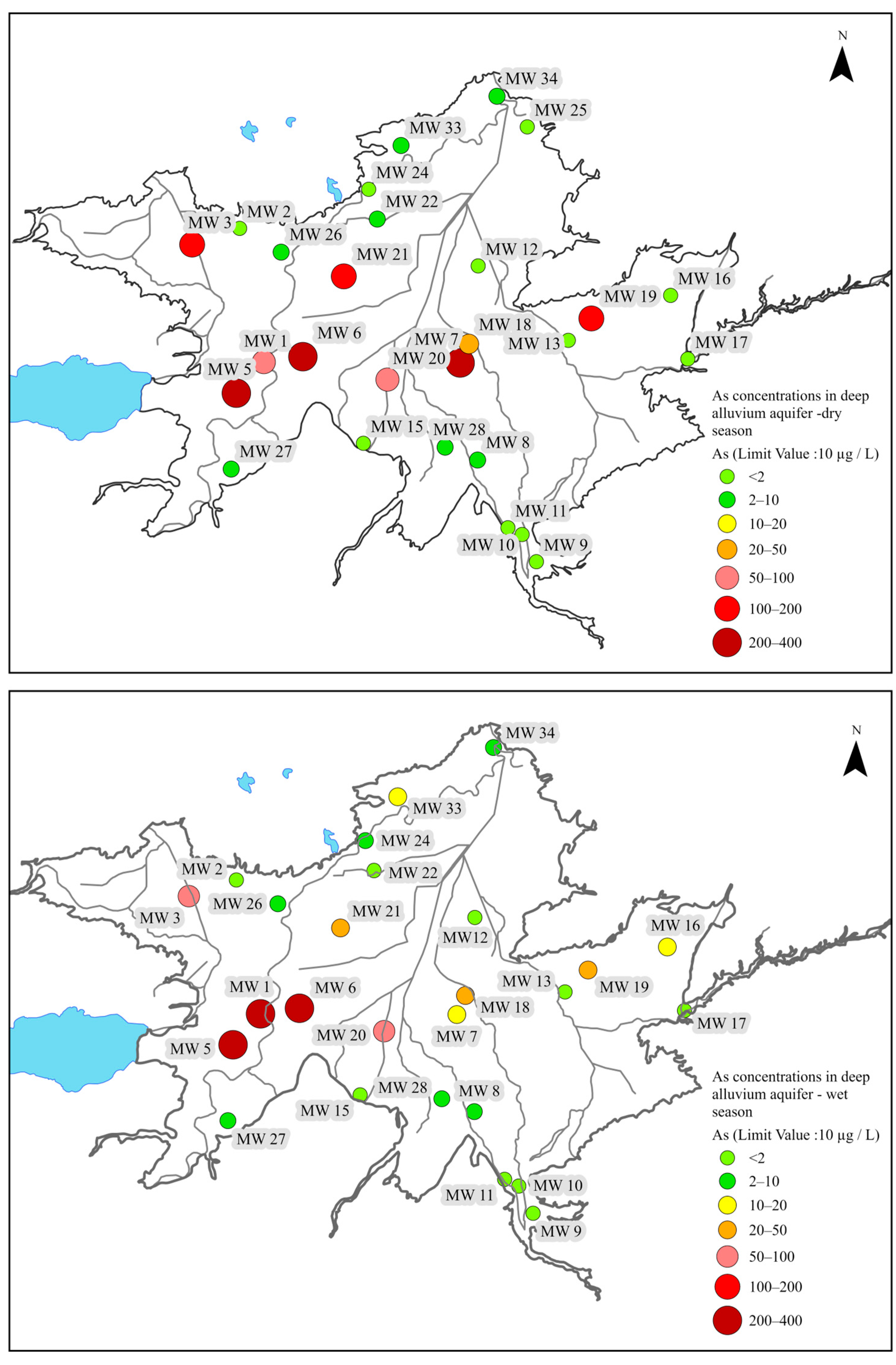
6.1.2. Deep Alluvium Aquifer

Deep alluvial aquifer groundwater exhibits mostly alkaline character with a mean pH value of 7.67 ± 0.58 (stdev), while approximately 19% of the groundwater samples show slight acidic character mostly in dry period. The electrical conductivity values vary from 168 to 2828 µS/cm with a mean value of 882.36 µS/cm ± 566.29 (stdev). About 30–37% of the groundwater samples exhibit high EC values above 1000 µS/cm. Although mean dissolved oxygen (DO) concentrations in the deep aquifer were moderate—6.02 ± 3.27 mg/L during the dry season and 5.46 ± 3.09 mg/L during the wet season—30–37% of the samples recorded DO levels between 1.15 and 3.3 mg/L in both periods. This indicates the coexistence of oxic and suboxic conditions within the deep aquifer.

Calcium (Ca²⁺) was the dominant cation in 36–43% of the samples depending on the season, while sodium (Na⁺) dominated in 14–22% (

Table A5. Physicochemical properties of groundwater collected from the deep aquifer for the dry season in the Lower Sakarya Plain (September 2018).

Sample No	pH	DO	EC	Na+	K+	Ca2+	Mg2+	Cl−	SO42−	HCO3−	F−	NO3−
		mg/L	µS/cm at 25 °C	mg/L	mg/L	mg/L	mg/L	mg/L	mg/L	mg/l	mg/L	mg/L
MW 1	7.82	1.45	1292.20	126.09	3.91	43.88	38.89	78.87	0.20	450.25	0.36	0.21
MW 2	6.27	4.68	647.50	26.15	1.49	48.16	12.48	70.89	26.09	118.07	0.25	13.25
MW 3	7.03	1.46	1523.20	160.21	11.62	58.60	61.38	62.30	83.13	629.45	0.45	0.23
MW 5	7.54	1.76	1705.20	142.86	5.18	64.87	94.23	59.44	0.20	891.41	0.40	0.29
MW 6	7.95	9.31	1535.80	100.48	5.22	97.12	98.67	18.36	0.20	809.56	0.34	0.11
MW 7	7.57	1.34	1212.40	95.88	1.29	70.48	34.87	9.51	6.53	607.13	0.28	0.10
MW 8	7.54	2.26	487.76	17.62	1.19	35.57	15.73	4.15	14.01	224.92	0.25	0.57
MW 9	6.89	7.15	833.00	26.01	2.76	92.52	19.82	37.46	12.82	357.18	0.21	16.62
MW 10	7.37	6.87	749.00	23.93	1.66	67.25	17.37	32.78	34.90	268.62	0.21	12.14
MW 11	7.75	8.00	564.20	13.54	1.18	58.06	12.62	9.70	27.15	226.38	0.23	7.58
MW 12	7.42	6.34	580.58	21.26	1.47	53.45	16.92	18.29	24.63	238.73	0.23	5.66
MW 13	8.16	6.80	661.08	39.81	0.76	55.61	11.70	18.90	4.72	305.21	0.31	0.60
MW 15	8.14	3.09	576.80	77.11	0.78	28.12	2.44	28.32	0.20	232.85	0.16	0.10
MW 16	7.16	4.82	491.12	53.27	0.61	26.25	6.06	16.94	16.35	186.39	0.27	3.90
MW 17	7.82	12.49	327.36	1.98	0.36	35.40	5.75	1.96	4.86	134.41	0.17	2.26
MW 18	6.71	6.01	2296.60	128.90	6.28	171.30	117.49	9.76	0.18	1213.28	0.29	1.18
MW 19	7.62	3.65	992.60	58.12	2.38	68.08	32.88	12.21	0.20	538.82	0.33	0.47
MW 20	7.39	4.39	1926.40	128.20	1.63	141.73	79.96	5.74	0.20	1015.59	0.38	0.25
MW 21	7.87	8.04	1160.60	86.19	4.65	48.25	66.35	17.42	0.34	642.44	0.59	0.08
MW 22	8.10	9.44	289.38	9.08	1.52	33.43	7.85	10.53	15.11	119.52	0.20	1.38
MW 24	6.44	10.60	924.00	5.71	0.16	21.07	2.76	1.45	9.07	78.06	0.17	2.25
MW 25	6.24	6.24	168.00	4.29	0.08	18.61	2.20	1.36	5.57	63.06	<0.15	2.55
MW 26	8.44	11.10	1242.80	103.99	5.54	46.03	76.05	23.67	14.95	626.26	0.26	0.68
MW 27	8.04	9.52	908.60	8.53	1.36	30.92	7.39	10.56	0.20	108.73	0.14	0.72
MW 28	7.56	3.33	554.80	15.16	1.49	39.39	12.94	6.87	15.70	247.86	0.16	0.08
MW 33	8.61	2.29	270.90	8.78	1.42	32.60	7.60	11.22	14.95	108.19	0.12	0.46
MW 34	7.92	10.10	267.80	8.86	1.44	33.00	7.77	10.73	15.05	116.03	0.13	0.52
Min	6.24	1.34	168.00	1.98	0.08	18.61	2.20	1.36	0.18	63.06	0.12	0.08
Max	8.61	12.49	2296.60	160.21	11.62	171.30	117.49	78.87	83.13	1213.28	0.59	16.62
Mean	7.53	6.02	895.91	55.26	2.50	56.29	32.23	21.83	17.39	391.05	0.27	2.96
STDV	0.61	3.27	539.08	49.94	2.49	34.55	33.72	21.30	16.84	309.29	0.11	4.40

and

Table A6. Physicochemical properties of groundwater collected from the deep aquifer for the wet season in the Lower Sakarya Plain (April 2019).

Sample No	pH	DO	EC	Na+	K+	Ca2+	Mg2+	Cl−	SO42−	HCO3−	F−	NO3−
		mg/L	µS/cm at 25 °C	mg/L	mg/L	mg/L	mg/L	mg/L	mg/L	mg/l	mg/L	mg/L
MW 1	7.47	1.73	1464.40	74.91	4.84	63.98	58.03	49.03	0.20	661.97	0.46	0.60
MW 2	6.09	7.73	524.40	22.92	1.46	41.62	11.35	103.30	24.10	82.34	0.19	19.60
MW 3	7.98	4.54	1209.60	118.42	15.50	28.53	29.34	53.11	78.16	508.27	0.33	4.04
MW 5	8.04	7.49	2828.00	310.54	8.64	47.28	87.20	134.69	1.41	1429.38	0.74	0.88
MW 6	7.73	7.73	1541.40	78.43	4.50	95.18	85.61	21.53	0.20	875.64	0.31	0.48
MW 7	8.20	2.12	1288.00	78.92	1.24	50.73	19.05	11.53	4.01	533.69	0.31	0.62
MW 8	8.32	1.94	483.28	15.28	1.11	33.94	14.01	5.65	16.64	213.78	0.25	0.87
MW 9	7.55	6.8	666.26	14.69	1.65	66.53	12.28	23.41	18.89	279.00	0.17	26.99
MW 10	8.07	10.06	547.40	11.09	1.07	50.63	11.94	13.74	33.08	216.44	0.25	9.96
MW 11	7.90	9.66	1027.60	42.13	2.47	91.79	16.41	49.36	28.68	395.55	0.18	16.83
MW 12	8.08	4.45	436.80	14.65	1.07	37.06	13.13	7.93	17.69	229.28	0.27	0.80
MW 13	7.37	3.85	650.02	35.64	0.65	52.26	9.80	22.77	6.20	301.36	0.32	0.10
MW 15	8.34	2	588.98	63.74	0.65	19.40	2.00	35.64	0.20	232.56	0.10	1.01
MW 16	7.19	2.96	487.06	53.72	0.94	23.98	9.13	22.42	22.23	182.72	0.31	3.88
MW 17	7.86	7.11	380.80	1.67	0.30	35.20	4.57	3.11	8.00	134.81	0.13	2.89
MW 18	7.97	2.16	656.32	55.79	1.09	25.88	10.54	48.05	1.11	256.24	0.35	0.10
MW 19	8.18	4.8	1192.80	82.80	1.22	51.77	19.76	11.81	4.11	509.07	0.30	3.08
MW 20	7.23	1.15	1887.20	82.09	1.82	145.03	44.04	8.55	0.20	979.82	0.37	0.56
MW 21	8.42	7.66	833.00	45.06	3.67	32.85	39.22	16.02	2.18	449.55	0.66	0.70
MW 22	8.40	7.15	232.80	4.79	1.11	19.07	3.98	7.97	17.04	81.64	0.14	2.13
MW 24	7.30	11.6	252.00	5.32	0.99	20.41	4.56	9.66	17.42	81.21	0.18	1.60
MW 25	7.34	5.09	388.00	7.62	2.26	33.64	8.78	11.41	11.01	142.31	0.16	2.27
MW 26	7.60	3.3	1513.10	91.58	5.39	50.04	73.17	31.05	0.20	664.44	0.34	0.65
MW 27	8.32	10.39	253.00	7.01	1.28	24.12	5.79	13.68	19.16	110.65	0.19	1.32
MW 28	7.87	2.06	612.20	13.08	1.49	38.93	11.82	8.79	0.20	245.47	0.24	0.83
MW 33	7.43	2.42	1143.75	21.59	2.35	91.90	50.34	12.51	13.04	576.72	0.44	5.48
MW 34	8.35	9.36	369.60	6.51	1.24	24.39	5.50	13.67	18.82	125.53	0.20	2.82
Min	6.09	1.15	232.80	1.67	0.30	19.07	2.00	3.11	0.20	81.21	0.10	0.10
Max	8.42	11.60	2828.00	310.54	15.50	145.03	87.20	134.69	78.16	1429.38	0.74	26.99
Mean	7.80	5.46	868.81	50.37	2.59	48.01	24.49	27.79	13.49	388.87	0.29	4.11
STDV	0.51	3.09	591.94	60.62	3.11	28.65	24.92	29.81	15.97	314.69	0.15	6.51

). Meanwhile, 43–50% of the samples exhibited no dominant cation facies. With the exception of one sample where chloride was the dominant anion, bicarbonate (HCO₃⁻) was the predominant anion in all other samples (Figure 4). The average concentrations of calcium, chloride, and sulfate in deep groundwater are approximately 1.7, 2.5, and 7.5 times lower, respectively, than those in shallow aquifer groundwater (Table A1, Table A2, Table A5 and Table A6).

The deep alluvial aquifer, situated at depths exceeding 60 m, was notably impacted by arsenic (As) and manganese (Mn) contamination. Depending on the sampling period, As and Mn concentrations exceeded their respective drinking water limits (10 µg/L for As and 50 µg/L for Mn) in 33–41% and 44% of the samples, respectively. Groundwater from this aquifer exhibited pronounced seasonal variability in concentration. Arsenic concentrations above the maximum contaminant level ranged from 39.50 to 300.52 µg/L during the dry season and from 10.38 to 373.09 µg/L during the wet season (

Table A7. Descriptive statistics of trace element contents of groundwater samples collected from the deep aquifer in the Lower Sakarya Plain for the dry season (September 2018).

Sample No	Al	As	Ba	Cd	Co	Cr	Cu	Fe	Mn	Mo	Ni	Pb	Sb	Se	Sn	U	V	Zn
	µg/L	µg/L	µg/L	µg/L	µg/L	µg/L	µg/L	µg/L	µg/L	µg/L	µg/L	µg/L	µg/L	µg/L	µg/L	µg/L	µg/L	µg/L
MW 1	2.32	72.26	218.33	0.02	0.41	4.89	0.53	<5	72.60	6.27	3.01	0.02	2.80	0.07	1.63	0.004	1.17	2.47
MW 2	4.42	0.83	84.02	0.03	0.17	1.64	0.12	<5	15.60	0.02	4.18	0.07	2.52	0.46	0.03	0.38	0.99	28.84
MW 3	8.38	178.87	144.49	0.03	0.79	7.19	1.44	25.20	179.50	10.23	7.97	0.28	5.11	0.19	<0.01	1.14	4.24	1.39
MW 5	0.32	300.52	736.89	0.04	1.53	15.96	0.57	<5	83.40	13.52	13.00	<0.01	6.11	0.12	0.07	0.01	0.69	8.21
MW 6	4.80	300.18	214.42	0.03	0.86	12.22	2.81	<5	72.49	0.59	8.26	0.39	1.80	0.13	<0.01	0.01	0.27	17.21
MW 7	2.77	251.34	77.46	<0.01	0.47	5.37	1.30	<5	241.95	1.98	4.25	0.19	2.15	0.08	<0.01	0.02	0.38	2.32
MW 8	3.34	3.76	32.23	<0.01	0.12	2.14	<0.1	<5	103.16	1.44	1.76	0.11	0.25	0.06	<0.01	0.41	0.48	3.38
MW 9	1.90	0.71	25.88	<0.01	0.22	4.78	3.16	<5	1.55	0.13	5.97	0.02	0.76	0.05	<0.01	0.77	1.52	6.38
MW 10	3.54	0.64	71.46	<0.01	0.17	3.61	0.47	<5	0.55	0.33	3.78	0.31	0.62	0.30	<0.01	0.71	0.95	16.20
MW 11	1.56	0.37	45.40	<0.01	0.14	2.70	<0.1	<5	0.11	0.45	3.07	0.24	0.46	0.07	<0.01	0.54	0.74	1.53
MW 12	1.25	1.84	53.32	<0.01	0.14	2.28	0.27	<5	49.25	0.88	2.70	<0.01	0.37	0.13	<0.01	0.54	0.76	3.63
MW 13	1.54	1.72	29.57	<0.01	0.14	3.49	5.16	<5	91.40	3.58	2.85	1.05	0.72	0.27	<0.01	0.88	2.23	13.31
MW 15	4.19	1.41	42.20	0.02	0.10	2.54	1.00	<5	18.99	1.83	1.77	0.36	0.38	0.25	<0.01	0.01	0.41	2.65
MW 16	4.80	0.78	25.08	0.03	0.22	2.28	1.68	<5	51.27	9.92	2.43	0.08	0.90	0.08	<0.01	0.68	0.70	340.96
MW 17	16.46	0.26	9.89	<0.01	0.09	1.86	24.34	<5	1.27	0.22	4.15	0.84	0.30	0.07	<0.01	0.35	0.57	85.05
MW 18	<0.1	39.49	328.63	<0.01	1.05	65.24	1.08	<5	153.89	0.18	11.29	0.33	4.11	0.05	<0.01	0.02	0.15	14.99
MW 19	27.54	139.60	52.54	0.02	0.51	3.97	0.52	<5	209.26	5.22	6.36	0.03	1.26	0.26	<0.01	0.01	0.08	27.43
MW 20	5.03	91.91	207.84	<0.01	0.95	11.73	2.49	<5	214.73	1.41	17.43	0.09	4.05	0.14	<0.01	0.05	0.91	64.64
MW 21	8.96	133.32	354.48	0.08	0.40	4.74	3.20	<5	26.25	23.15	7.95	0.03	2.07	0.30	0.17	0.05	0.23	15.14
MW 22	28.78	3.89	10.50	<0.01	0.08	0.79	3.99	<5	0.22	0.33	3.04	0.12	0.34	0.13	<0.01	0.42	0.07	9.49
MW 24	7.41	0.58	17.79	<0.01	0.05	1.12	0.24	<5	0.10	0.37	0.84	0.14	0.48	0.10	<0.01	0.09	5.27	6.09
MW 25	4.45	0.26	0.79	<0.01	0.06	1.34	<0.1	<5	0.02	0.20	0.63	0.21	0.40	0.08	<0.01	0.04	11.11	2.44
MW 26	6.78	5.43	152.04	<0.01	0.17	7.81	13.03	<5	1.08	1.87	4.88	0.04	3.58	0.72	0.04	0.03	0.24	7.87
MW 27	7.90	3.00	9.98	<0.01	0.10	1.43	1.26	<5	1.74	0.33	2.17	0.07	0.43	0.30	<0.01	0.33	0.02	109.16
MW 28	3.93	6.79	37.39	<0.01	0.12	2.27	0.10	<5	147.70	0.77	1.80	0.12	0.25	0.20	<0.01	0.004	0.01	57.11
MW 33	17.15	3.58	9.06	<0.01	0.09	1.09	2.61	<5	0.59	0.28	2.06	<0.01	0.57	0.34	0.09	0.34	0.08	8.74
MW 34	12.08	3.76	9.17	<0.01	0.09	0.93	4.21	<5	1.19	0.29	4.30	0.35	0.65	0.31	0.08	0.35	0.06	49.97
Min	<0.1	0.26	0.79	<0.01	0.05	0.79	0.10	<5	0.02	0.02	0.63	<0.01	0.25	0.05	<0.01	0.004	0.01	1.39
Max	28.78	300.52	736.89	0.08	1.53	65.24	24.34	25.19	241.95	23.15	17.43	1.05	6.11	0.72	1.63	0.004	11.11	340.96
Mean	7.37	57.30	111.14	0.03	0.34	6.50	3.15	-	64.44	3.18	4.89	0.23	1.61	0.19	0.30	0.30	1.27	33.58
STDV	7.31	94.20	155.99	0.02	0.37	12.11	5.15	-	76.22	5.26	3.87	0.25	1.63	0.15	0.54	0.32	2.28	66.14

and

Table A8. Descriptive statistics of trace element contents of groundwater samples collected from the deep aquifer in the Lower Sakarya Plain for the wet season (April 2019).

Sample No	Al	As	Ba	Cd	Co	Cr	Cu	Fe	Mn	Mo	Ni	Pb	Sb	Se	Sn	U	V	Zn
	µg/L	µg/L	µg/L	µg/L	µg/L	µg/L	µg/L	µg/L	µg/L	µg/L	µg/L	µg/L	µg/L	µg/L	µg/L	µg/L	µg/L	µg/L
MW 1	<0.1	250.07	503.03	0.05	1.02	0.82	1.04	<1	63.09	8.89	8.06	0.11	0.86	4.27	0.11	0.002	0.56	24.63
MW 2	<0.1	0.74	103.26	0.07	0.12	0.69	0.30	<1	10.11	0.04	5.03	<0.01	0.76	2.38	0.09	0.11	1.14	49.25
MW 3	<0.1	77.59	100.93	0.04	0.64	44.83	1.87	<1	15.92	10.59	4.62	0.03	3.19	5.45	0.26	0.39	10.24	30.70
MW 5	2.53	373.09	479.80	0.10	0.99	26.04	2.36	<1	5.65	20.25	15.01	0.52	0.83	9.19	0.42	0.01	1.51	19.46
MW 6	<0.1	219.49	210.05	0.02	0.85	4.61	0.95	<1	59.85	0.61	8.35	0.01	0.94	1.85	0.27	0.02	0.36	13.21
MW 7	<0.1	18.37	184.82	0.01	0.50	6.33	0.40	<1	111.55	1.83	4.88	<0.01	1.15	2.48	2.33	0.01	0.14	7.89
MW 8	<0.1	3.12	29.28	0.01	0.12	4.30	0.76	<1	93.86	1.34	2.72	0.18	0.65	0.13	0.08	0.39	0.51	2.15
MW 9	<0.1	0.61	20.54	<0.01	0.20	2.88	0.32	<1	0.29	0.13	5.44	0.09	0.74	0.33	0.03	0.62	1.42	1.90
MW 10	<0.1	0.35	36.97	0.01	0.14	2.25	0.31	<1	0.11	0.35	4.02	0.04	0.62	0.29	0.01	0.55	0.95	1.81
MW 11	<0.1	0.56	82.92	0.01	0.25	7.42	0.39	<1	4.52	0.38	6.38	0.02	0.80	0.42	0.01	0.62	0.94	3.60
MW 12	<0.1	1.71	29.99	0.01	0.13	0.21	0.34	<1	65.61	1.28	2.67	0.04	0.77	0.03	0.06	0.39	0.48	10.61
MW 13	<0.1	1.50	28.76	0.04	0.20	0.20	0.26	<1	189.36	3.36	3.97	0.06	0.13	0.55	0.04	0.73	2.34	3.11
MW 15	<0.1	1.22	36.78	0.01	0.08	5.88	0.22	18.39	16.73	1.77	1.71	<0.01	0.52	0.38	<0.01	0.002	0.52	1.27
MW 16	<0.1	11.28	50.38	0.06	1.05	1.06	0.86	<1	161.12	8.10	5.02	0.02	0.23	0.87	0.34	0.57	0.60	359.51
MW 17	<0.1	0.26	12.41	<0.01	0.09	3.57	0.95	<1	0.00	0.23	2.38	0.37	0.70	0.12	0.01	0.32	0.50	5.30
MW 18	<0.1	30.55	57.69	0.02	0.23	4.22	0.17	<1	36.16	2.29	2.15	0.03	0.63	1.03	0.06	0.01	0.73	5.14
MW 19	<0.1	21.14	179.37	0.01	0.50	15.18	0.60	<1	111.40	1.83	4.78	<0.01	1.08	2.06	2.32	0.01	0.13	11.03
MW 20	<0.1	56.92	214.61	0.02	0.59	7.75	0.65	<1	317.90	2.51	11.53	0.02	0.63	2.39	0.08	0.01	0.11	7.97
MW 21	<0.1	35.62	262.16	0.06	0.49	8.63	1.53	<1	18.33	17.53	5.32	0.16	0.76	1.21	0.12	0.01	0.24	2057.47
MW 22	13.64	1.41	7.19	0.02	0.06	2.14	1.13	<1	0.36	0.50	1.90	0.05	0.63	0.32	0.18	0.19	1.96	8.07
MW 24	23.10	2.25	7.04	<0.01	0.07	0.46	0.76	<1	0.19	0.39	1.94	0.03	0.75	0.14	0.03	0.29	1.19	5.56
MW 25	<0.1	0.17	75.05	<0.01	0.34	0.43	0.41	<1	47.55	0.20	2.92	<0.01	0.72	0.15	0.03	0.11	0.11	5.33
MW 26	<0.1	7.31	279.32	0.01	0.26	2.72	2.37	<1	173.17	1.76	4.72	0.04	0.93	3.29	0.18	0.02	0.29	12.10
MW 27	2.91	3.75	8.58	<0.01	0.08	1.92	0.88	<1	0.57	0.27	2.64	0.07	0.76	0.61	0.12	0.41	0.19	9.48
MW 28	<0.1	6.68	36.95	0.01	0.13	6.36	0.55	<1	140.49	0.76	3.31	<0.01	0.74	0.17	<0.01	0.001	0.12	35.31
MW 33	<0.1	10.38	132.61	0.02	2.11	16.00	0.27	<1	1228.79	4.27	9.34	0.02	0.74	0.50	0.21	0.90	0.28	120.53
MW 34	26.47	3.11	8.68	0.01	0.09	1.18	9.39	<1	0.26	0.29	2.67	0.59	0.85	0.36	0.45	0.35	0.26	10.44
Min	<0.1	0.17	7.04	<0.01	0.06	0.20	0.17	<1	0.00	0.04	1.71	<0.01	0.13	0.03	<0.01	0.001	0.11	1.27
Max	26.47	373.09	503.03	0.10	2.11	44.83	9.39	18.39	1228.79	20.25	15.01	0.59	3.19	9.19	2.33	0.90	10.24	2057.47
Mean	13.73	42.19	117.75	0.023	0.42	6.60	1.11	-	106.41	3.40	4.94	0.12	0.82	1.52	0.31	0.26	1.03	104.55
STDV	9.93	89.12	132.84	0.024	0.45	9.44	1.73	-	233.09	5.17	3.10	0.16	0.51	2.03	0.61	0.26	1.90	389.14

; Figure 6 and Figure 7). Similarly, Mn concentrations ranged from 51.27 to 241.95 µg/L in the dry season and varied substantially in the wet season, reaching values between 59.85 and 1228.79 µg/L.

Around 30–33% of the wells sampled in both periods showed elevated arsenic and manganese concentrations, exceeding their respective MCLs. These wells typically had very low sulfate levels (0.2–2 mg/L) alongside high bicarbonate concentrations (450–1429 mg/L). In several cases, dissolved oxygen levels were also notably low (1.45–3.3 mg/L). Additionally, iron concentrations were consistently low, remaining below the detection limit in nearly all samples. These results suggest that the rise in arsenic levels in conjunction with the observed geochemical conditions is likely driven by localized reducing redox conditions within an otherwise moderately oxic deep alluvial aquifer. In such redox windows—intermediate between oxic and strongly reducing conditions—arsenic is typically released through the reductive dissolution of iron and manganese oxyhydroxides, which are major sinks for arsenic in aquifer sediments. Smedley and Kinniburgh (2002) [1] and Shaji et al. (2021) [6] consistently highlight the reductive dissolution of iron and manganese oxides as the dominant geochemical mechanism driving arsenic mobilization in natural groundwater systems. Both studies emphasize that manganese oxides, due to their higher redox sensitivity, undergo dissolution under mildly reducing conditions prior to iron oxides, initiating the release of adsorbed arsenic and trace metals. As redox conditions reduce further, iron oxides—typically the primary geochemical sink for arsenic—also dissolve, further amplifying arsenic mobility. Together, these sequential processes illustrate the coupled role of Mn and Fe cycling in regulating arsenic release across a wide range of aquifer environments globally.

The low sulfate levels across these wells also reflect a history of sulfate reduction, further contributing to the development of sulfate-reducing conditions. Under sulfate-reducing conditions, Fe²⁺ released through the reductive dissolution of Fe(III) (oxyhydr)oxides may precipitate rapidly as iron sulfide minerals, which can be likely mechanism for the absence of iron in these wells despite high manganese concentrations. This mechanism is well-supported by Smedley and Kinniburgh (2002) [1], who emphasized that the reductive dissolution of iron (oxyhydr)oxides releases Fe²⁺, which may subsequently precipitate as sulfide minerals in the presence of sulfide ions. Similarly, Shaji et al. (2021) [6] noted that such conditions—common in organic-rich, alluvial aquifers affected by geogenic arsenic—are conducive not only to the mobilization of arsenic and manganese, but also to the suppression of aqueous iron via mineral precipitation. Together, these findings underscore the complex interplay between microbial sulfate reduction, redox dynamics, and the selective solubility of redox-sensitive metals in groundwater systems.

Smedley and Kinniburgh (2002) and Shaji et al. (2021) [1,6] also highlight that elevated bicarbonate concentrations can play a critical role in enhancing arsenic mobility in groundwater systems. Under neutral to alkaline pH conditions, bicarbonate ions compete with arsenic oxyanions for adsorption sites on mineral surfaces, particularly iron oxides. This competition reduces the surface retention of arsenic, promoting its release into the aqueous phase. Such mechanisms are frequently observed in alluvial aquifers where high bicarbonate levels often correlate with increased dissolved arsenic, underscoring the influence of carbonate chemistry on arsenic transport and availability [1,6,30].

On the other hand, a different pattern was observed in two specific wells, MW16 and MW33. While arsenic concentrations in these wells were below the permissible limit during the dry season (0.78 µg/L and 3.58 µg/L), they elevated significantly during the wet season to 11.28 µg/L and 10.33 µg/L, exceeding the MCL. This increase was also accompanied by elevated manganese levels (161 µg/L and 1229 µg/L) (Table A7 and Table A8, Figure 6 and Figure 7).

Unlike the other high-As and Mn containing wells, MW16 and MW33 exhibited moderately higher sulfate concentrations (14.95–22.23 mg/L). However, DO levels remained low, ranging between 2.42 and 2.96 mg/L. These exceptions highlight the complex and spatially variable geochemical processes influencing arsenic and manganese mobilization within the aquifer, while reinforcing their frequent co-occurrence in affected zones.

Nitrate (NO₃) concentrations in the deeper aquifer were significantly lower compared to those in the shallow alluvial aquifer. The average nitrate concentrations in deep aquifer groundwater ranged from 0.90 to 1.83 mg/L during the dry and wet periods (Table A5 and Table A6). In the dry period, nitrate levels in three wells (MW 2, MW 9, and MW 10) out of 27 samples ranged from 12.14 to 16.62 mg/L, with MW 9 recording the highest concentration of 16.62 mg/L. During the wet period, although nitrate concentrations remained within permissible limits, elevated nitrate levels were observed in wells MW 2, MW 9, MW 10, and MW 11, ranging from 16.83 to 26.99 mg/L (Figure 5; Table A5 and Table A6). These elevated nitrate concentrations, exceeding the average background levels in the deep alluvial aquifer, suggest a localized hydraulic connection between the shallow and deep alluvial aquifers and the moderate pressure of agricultural activities on the water quality.

Figure 6. Dot distribution of Mn concentrations in shallow and deep alluvium aquifers in both dry and wet seasons.

Figure 6. Dot distribution of Mn concentrations in shallow and deep alluvium aquifers in both dry and wet seasons.

Figure 7. Dot distribution of As concentrations in the deep alluvium aquifer in both dry and wet seasons.

Figure 7. Dot distribution of As concentrations in the deep alluvium aquifer in both dry and wet seasons.

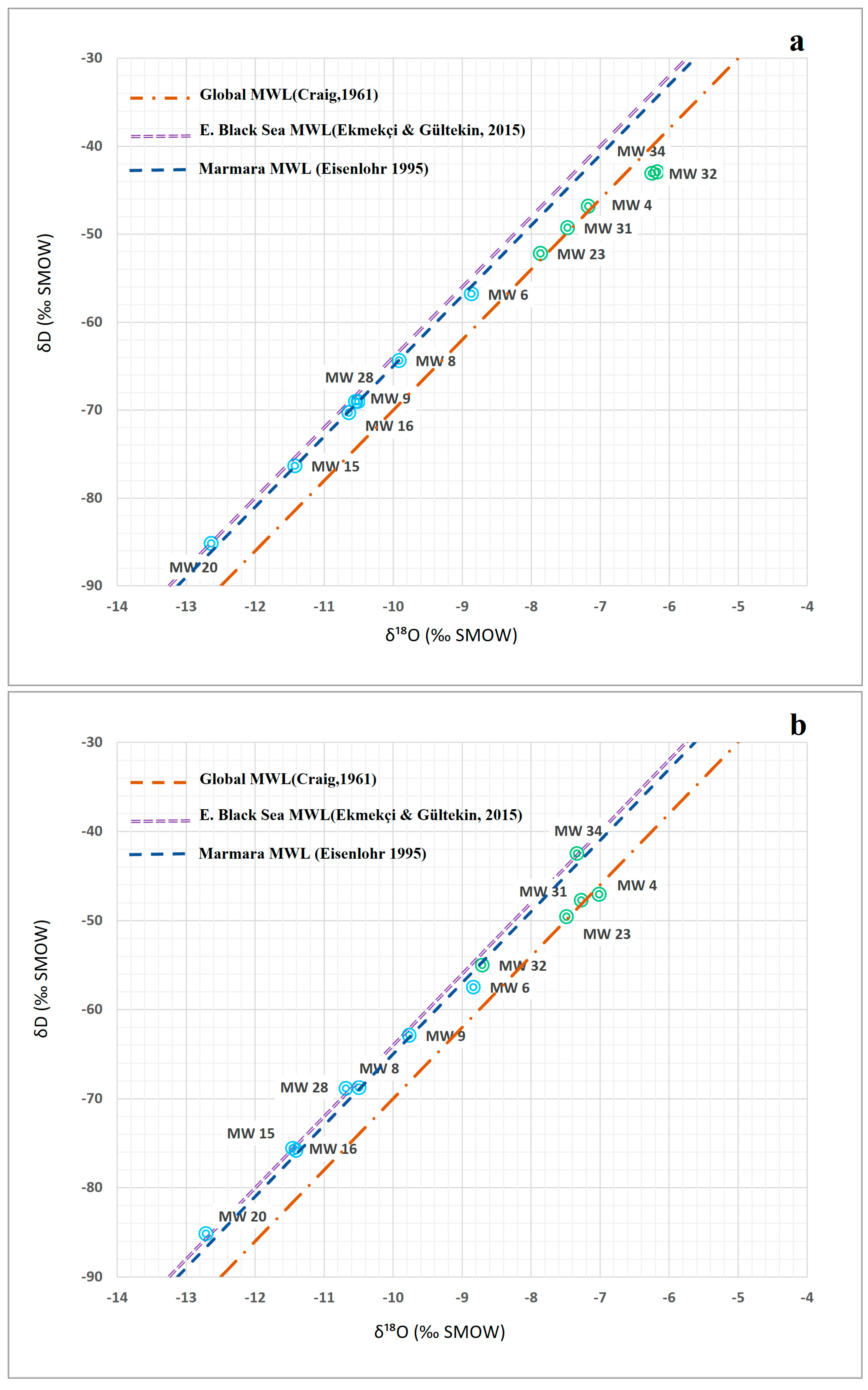
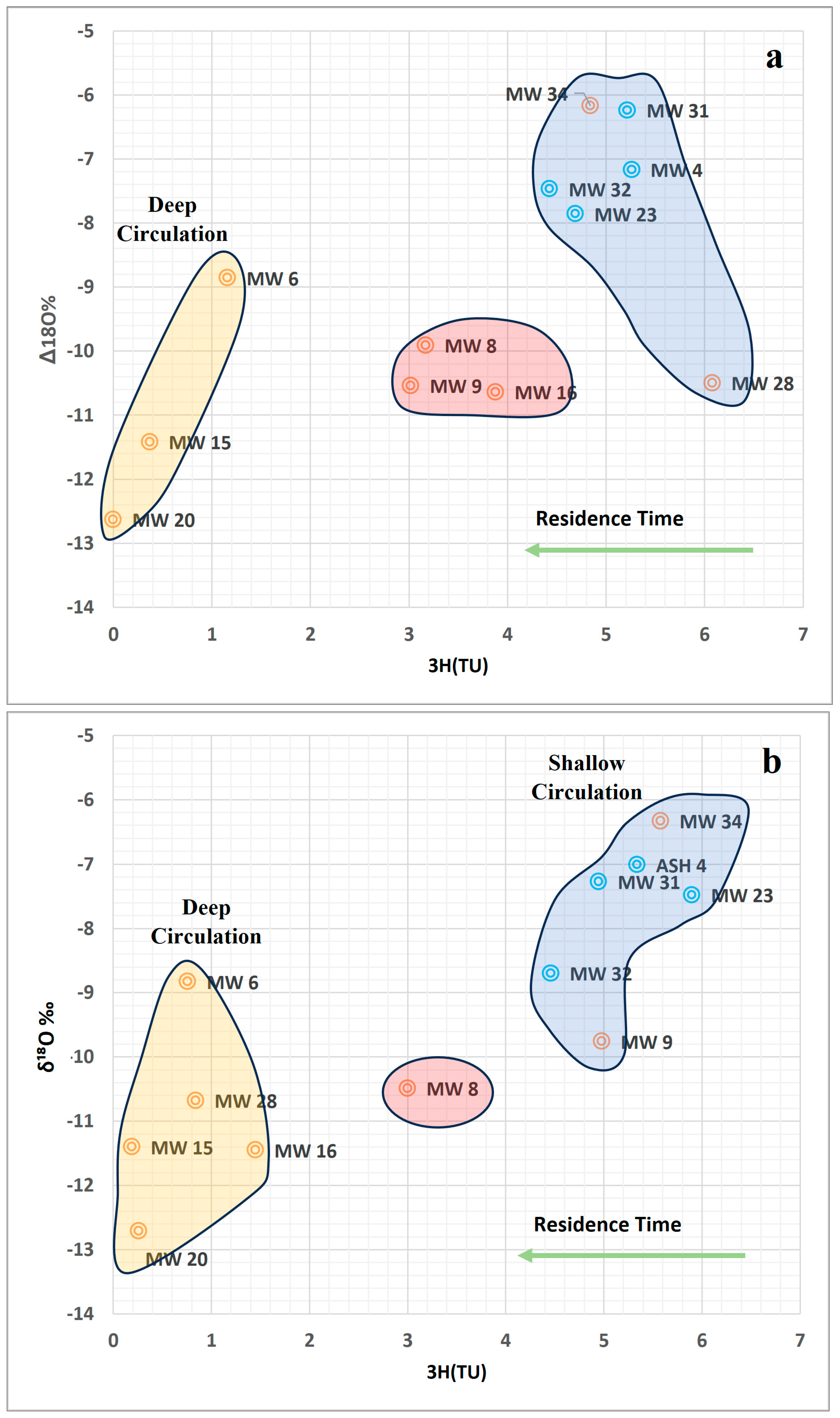
6.2. Assessment of Isotopic Characteristics of Alluvium Aquifer

To determine groundwater residence times and the possible hydraulic connection between shallow and deep alluvial aquifers, stable isotope and tritium concentrations of the selected well samples from shallow and deep aquifers were measured at both dry and wet periods (

Table A9. Environmental isotope analysis results of the groundwater samples for dry and wet seasons from the alluvial aquifer in the Lower Sakarya Basin.

Sample No	X Easting	Y Northing	Elevation (m)	Well Depth (m)	Deuterium (δD, ‰)		Oxygen-18 (δ18O, ‰)		Tritium (TU)		D-Excess
					Sep-18	Apr-19	Sep-18	Apr-19	Sep-18	Apr-19	Sep-18	Apr-19
MW 4	280558	4518352	32	36.0	−46.84	−47.04	−7.17	−7.01	5.26	5.34	10.52	9.04
MW 6	284453	4513591	30	102.0	−56.83	−57.5	−8.86	−8.83	1.16	0.76	14.05	13.14
MW 8	295482	4507074	4	94.0	−64.39	−68.79	−9.91	−10.49	3.17	3.00	14.89	15.13
MW 9	299200	4500659	42	107.00	−69.05	−62.94	−10.54	−9.76	3.02	4.98	15.27	15.14
MW 15	287913	4512153	40	102.00	−76.36	−75.87	−11.42	−11.4	0.37	0.19	15.00	15.33
MW 16	307667	4517462	14	106.00	−70.33	−75.61	−10.64	−11.45	3.88	1.45	14.79	15.99
MW 20	289797	4512153	28	112.00	−85.2	−85.2	−12.63	−12.71	0	0.26	15.84	16.48
MW 23	277363	4505896	42	24.00	−52.23	−49.62	−7.86	−7.48	4.69	5.9	10.65	10.22
MW 28	293438	4507889	45	72.00	−69.07	−68.88	−10.5	−10.68	6.08	0.84	14.93	16.56
MW 31	274752	4523782	22	28.00	−49.3	−47.74	−7.47	−7.27	4.43	4.95	10.46	10.42
MW 32	290203	4527168	25	22.00	−43.1	−55.04	−6.24	−8.7	5.22	4.46	6.82	14.56
MW 34	296679	4531796	33	65.00	−42.94	−42.52	−6.17	−7.33	4.84	5.58	6.42	16.12

, Figure 8 and Figure 9).

The distribution of groundwater samples in the δ²H–δ¹⁸O graphs for both the dry (Figure 8a) and wet (Figure 8b) seasons demonstrates a clear meteoric origin for both shallow and deep groundwater systems. Most samples closely follow the Eastern Black Sea Meteoric Water Line (δ²H = 8 × δ¹⁸O + 16) [31] and, to a lesser extent, the Marmara MWL(δ²H = 8 × δ¹⁸O + 15) [32], suggesting that the groundwater likely originates from precipitation derived from the Black Sea. Deep aquifer samples (blue circles), such as MW15, MW16, MW20, and MW28, consistently plot at the lower left of the diagrams with depleted δ¹⁸O values (−10.5 to −13‰) and δ²H values (−68 to −85‰), indicating recharge from higher altitudes and cooler climatic conditions. These samples remain relatively unchanged between seasons, reflecting their long residence times and hydrogeologic isolation from modern recharge. Shallow aquifer samples (green symbols), including MW4, MW23, MW31, MW32, and MW34, exhibit more enriched isotope values (δ¹⁸O between −7.9 and −6.14‰), suggesting lower elevation recharge under present-day conditions. Their clustering near the Eastern Black Sea MWL further supports modern, regionally consistent precipitation as the dominant source. The isotopic stability of most wells between seasons suggests that while recharge pathways differ by depth, they remain consistent throughout the year, with deep and shallow aquifers showing distinct but seasonally stable isotope signatures.

Deuterium excess (d-excess) values range from 6.4‰ to 16.6‰ across both seasons (Table A9). Deep aquifer samples consistently exhibit higher d-excess values (~14.05–16.6‰), indicating recharge from meteoric water with minimal evaporation. In contrast, shallow aquifer samples (MW4, MW23, MW31, MW32 and MW34) show significantly lower d-excess values (~6.4–10.65‰), suggesting partial isotopic enrichment due to evaporation prior to infiltration. These patterns highlight the influence of evaporation in the recharge of shallow unconfined aquifer.

The relationship between δ¹⁸O and tritium (³H) values provides valuable insight into the recharge elevation, residence time, and circulation patterns of groundwater in the study area (Figure 9a,b). In both the dry and wet seasons, groundwater samples cluster into three distinct groups. The orange-shaded zone represents deep circulation, composed of samples MW6, MW15, MW20, and in the wet season also MW28, with low tritium values (0–1.16 T.U.) and depleted δ¹⁸O values (−12.7 to −8.8‰). These characteristics indicate high-altitude recharge under cooler climatic conditions and long residence times, suggesting limited interaction with modern recharge. The blue-shaded zone reflects shallow circulation, including MW4, MW23, MW31, MW32, and MW34, with δ¹⁸O values between −7.8 and −6.0‰ and ³H concentrations around 4.4–5.9 T.U., consistent with low-elevation recharge and relatively short residence times. Finally, the red-shaded zone represents a transitional or mixed domain, including MW8, MW9, and MW16, with intermediate tritium values (3–3.88 T.U.) and δ¹⁸O values similar to those of deep water. These samples likely represent zones of mixing between modern and older recharged water. Except for MW9 and MW16 deep aquifer groundwater samples, showing significant seasonal variation, the seasonal comparison of the other well samples indicates that the groundwater circulation remains stable in both shallow and deep aquifers throughout the year.

Figure 8. Plot of δ18O vs. δD contents of selected groundwater samples in (a) the dry season and (b) the wet season showing samples that were located between the Global [33] and Eastern Black Sea MWL [31]. Blue circles represent the deep alluvial aquifer, and green circles represent shallow alluvium aquifer groundwater samples.

Figure 8. Plot of δ18O vs. δD contents of selected groundwater samples in (a) the dry season and (b) the wet season showing samples that were located between the Global [33] and Eastern Black Sea MWL [31]. Blue circles represent the deep alluvial aquifer, and green circles represent shallow alluvium aquifer groundwater samples.

Figure 9. Plots of tritium (TU) vs. δ18O contents of selected groundwater samples for (a) the dry season and (b) the wet season (blue circles represent the shallow aquifer, red circles represent deep alluvium aquifer groundwater samples).

Figure 9. Plots of tritium (TU) vs. δ18O contents of selected groundwater samples for (a) the dry season and (b) the wet season (blue circles represent the shallow aquifer, red circles represent deep alluvium aquifer groundwater samples).

In conclusion, stable isotope and tritium data offer valuable insight into the recharge dynamics of the alluvial aquifer system. Shallow groundwater reflects active and recent recharge from low-elevation precipitation, suggesting a close link to current hydrological conditions and relatively short residence times. In contrast, deep groundwater is characterized by older, high-altitude recharge and significantly longer residence, pointing to a slower and more isolated renewal process. These distinct patterns indicate a stratified recharge regime, with shallow and deep aquifers operating largely independently and maintaining stable circulation characteristics throughout the year.

6.3. Mineralogical and Geochemical Characterization of Alluvial Sediments

To investigate arsenic sources, alluvial sediment samples were collected from shallow and deeper levels of the alluvial aquifer during groundwater drilling in the Alancuma district, selected due to prior As-Mn enrichments in nearby wells (Figure 1). Groundwater drilling, conducted in May 2020 near the southwestern study boundary, reached a depth of 110 m. Two composite samples were collected: 0–50 m, comprising silty sandy clay, and 50–110 m, characterized by pebbles of different origin including ophiolitic rocks, serpentinite, quartzite, and limestone. The mineralogical and geochemical compositions of the composite core samples are presented in Figure 10 and

Table A10. Geochemical analyses of Alancuma core sediment samples.

Sampling Depths (m)	As	Mn	Cd	V	Al	Fe	Cr	Co	Ni	Cu	Zn	Mo	Pb	Tl	Sn	Sb	Se
	mg/kg	mg/kg	mg/kg	mg/kg	mg/kg	mg/kg	mg/kg	mg/kg	mg/kg	mg/kg	mg/kg	mg/kg	mg/kg	µg/kg	µg/kg	µg/kg	µg/kg
ALANCUMA (0–50 m)	8.2	577	0.1	16.3	5118	10,667	48.7	9.1	65.4	42.6	69.7	0.7	11.4	87.2	121	10.2	<1
ALANCUMA (50–110 m)	3.1	313	0.1	7.0	1940	4463	50.5	4.0	56.6	9.4	10.1	3.3	2.7	27.0	48.4	6.5	<1

.

XRD analyses revealed a diverse mineral composition in the alluvial aquifer, reflecting the complex geology of the region, which includes both ophiolitic rocks and metamorphic–felsic sources. XRD analysis of core samples taken from different depths of the alluvium reveals the presence of quartz and calcite and, to a lesser extent, muscovite, kaolinite-montmorillonite, albite, pargasite, clinochlore and gismondine (Figure 10). The high contents of quartz and calcite presence in the minerals suggest that alluvium includes materials derived from quartzite and marble basement rocks. The widespread presence of calcite also helps explain the dominance of calcium and bicarbonate-based water types observed in both shallow and deep groundwater. The existence of clinochlore, pargasite, and gismondine suggest a mafic to ultramafic protolith and indicate medium-grade metamorphism or hydrothermal alteration of mafic rocks. Their presence indicates that ultramafic and mafic rocks are contributing material to the alluvial deposits.

The Alancuma composite sediment samples, collected from depths of 0–50 m and 50–110 m, exhibited arsenic concentrations of 8.2 mg/kg and 3.1 mg/kg, respectively, while manganese concentrations ranged from 313 mg/kg to 577 mg/kg. Iron contents of the sediment samples also varied from 1.06% to 0.446% (Table A10). The concentrations of other metals also showed variation, with aluminum ranging from 0.51% to 0.19%, nickel from 65.4 to 56.6 mg/kg, and chromium from 48.7 to 50.5 mg/kg, respectively. These values represent the readily available (labile) fraction of metals within the alluvial sediments.

Despite the relatively higher presence of Fe and Mn in the labile fractions of the sediments, no secondary Fe or Mn oxides were identified in the XRD analysis. This is likely due to limitations in detection sensitivity, attributed to their low overall concentrations and/or poor crystallinity.

Elevated arsenic levels in sediment or groundwater are typically associated with iron oxides, which act as the primary geochemical sink due to their strong sorptive capacity. Manganese oxides, while less effective in direct arsenic retention, play a secondary role by oxidizing As(III) to As(V), indirectly affecting arsenic mobility and speciation [1].

Typical concentrations of arsenic in Fe and Mn oxides range from 0.01 to %1 and 10 to 1000 mg/kg, respectively. In the Alancuma alluvial sediments, minerals such as quartz, feldspar, and biotite contain trace amounts of arsenic, typically ranging from 0.4 to 1.4 mg/kg.

Carbonate minerals, including calcite and dolomite, also incorporate arsenic, with concentrations reaching up to 8 mg/kg and 3 mg/kg, respectively [1,34]. In addition to acting as minor arsenic hosts, these minerals—particularly calcite—may function as natural adsorbents in calcareous sedimentary environments, thereby playing a role in the retention and mobility of arsenic within the subsurface system. However, the absence of a correlation between arsenic and calcium in present study (see Section 6.4) implies that carbonate dissolution does not significantly contribute to arsenic mobilization in the deep aquifer.

In summary, the mineralogical and geochemical data from alluvial sediments suggest that arsenic mobility is primarily controlled by redox-driven interactions with iron and manganese-bearing phases. Although no crystalline Fe or Mn oxides were detected via XRD, the presence of significant labile Fe and Mn suggests that poorly crystalline or amorphous forms likely exist and govern arsenic dynamics.

6.4. Statistical Analysis of Groundwater Chemistry Data

A statistical analysis was conducted on the chemical analysis results of groundwater samples from the deep alluvium aquifer using Pearson’s rank correlation coefficient analysis. The results are presented in

Table A11. Pearson correlation coefficients between chemical variables (n = 27), obtained from dry period chemical analyses of the deep alluvial aquifer system.

Variables	Na	K	Ca	Mg	HCO3	Al	As	Ba	Co	Mn	Mo	Ni
Na	1
K	0.765 **	1
Ca	0.547 **	0.392 *	1
Mg	0.832 **	0.731 **	0.743 **	1
HCO3	0.861 **	0.647 **	0.835 **	0.957 **	1
Al	−0.273	−0.094	−0.263	−0.234	−0.250	1
As	0.686 **	0.532 **	0.344	0.663 **	0.655 **	−0.066	1
Ba	0.719 **	0.550 **	0.423 *	0.790 **	0.739 **	−0.293	0.664 **	1
Co	0.820 **	0.628 **	0.680 **	0.866 **	0.883 **	−0.218	0.783 **	0.858 **	1
Mn	0.579 **	0.323	0.532 **	0.450 *	0.624 **	−0.063	0.544 **	0.241	0.565 **	1
Mo	0.489 **	0.443 *	−0.068	0.349	0.330	−0.025	0.456 *	0.601 **	0.396 *	0.150	1
Ni	0.713 **	0.515 **	0.791 **	0.826 **	0.871 **	−0.107	0.574 **	0.713 **	0.869 **	0.499 **	0.319	1

* Correlation is significant at the 0.05 level (2-tailed). ** Correlation is significant at the 0.01 level (2-tailed).

and

Table A12. Pearson correlation coefficients between chemical variables (n = 27), obtained from wet period chemical analyses of the deep alluvial aquifer system.

Variables	Na	K	Ca	Mg	HCO3	As	Ba	Co	Mn	Mo	Ni
Na	1
K	0.631 **	1
Ca	0.168	0.041	1
Mg	0.691 **	0.551 **	0.508 **	1
HCO3	0.854 **	0.532 **	0.594 **	0.890 **	1
As	0.800 **	0.547 **	0.244	0.777 **	0.800 **	1
Ba	0.737 **	0.482 *	0.360	0.836 **	0.826 **	0.813 **	1
Co	0.385 *	0.332	0.439 *	0.600 **	0.563 **	0.458 *	0.520 **	1
Mn	−0.055	−0.051	0.448 *	0.262	0.218	−0.084	0.080	0.752 **	1
Mo	0.716 **	0.601 **	−0.054	0.521 **	0.584 **	0.638 **	0.665 **	0.473 *	0.018	1
Ni	0.728 **	0.412 *	0.693 **	0.794 **	0.905 **	0.742 **	0.755 **	0.681 **	0.352	0.565 **	1

* Correlation is significant at the 0.05 level (2-tailed). ** Correlation is significant at the 0.01 level (2-tailed).

.

The results of Pearson’s correlation analysis revealed a moderate correlation between arsenic and manganese, with a correlation coefficient of rdry = 0.54 during the dry season while poor correlation (rwet = −0.08) in the wet season (Table A11 and Table A12). Iron concentration in groundwater was very low and remained below the instrument’s detection limit in both dry and wet period, suggesting no correlation with arsenic.

Metal oxide mineral phases in sediments, particularly iron and manganese oxides and hydroxides, are known to be among the primary sources of arsenic due to strong adsorption of arsenic to these mineral surfaces [1]. Although Fe and Mn are present in labile fraction of the alluvial sediments, Fe and Mn oxides could not be detected in XRD analyses due to poor crystallinity and low abundances.

The moderate correlation between As and Mn at dry period water samples suggests that elevated As concentrations in the deep alluvial aquifer are likely associated with Mn oxides, which originate from undifferentiated metamorphic rocks and serpentines, as discussed in geology section. This is further supported by a robust correlation of As with Mg (rdry = 0.663, rwet = 0.777), Co (rdry = 0.783, rwet = 0.458) and Ni (rdry = 0.574, rwet = 0.742) (Table A11 and Table A12). Based on the observed correlation among elements and geology, Pokrovski et al. (2003) [35] and Faust (1996) [36] suggest that serpentinized ultramafic rocks and associated hydrous nickel–magnesium silicates may act as a geogenic source of arsenic. As shown by Faust (1966) [36], these minerals naturally incorporate Ni and Co within their crystal structures and are abundant in serpentinized ultrabasic intrusions. Additionally, Pokrovski et al. (2003) [35] demonstrated that arsenic can form stable complexes with Ni and Co under hydrothermal and water–rock interaction conditions, supporting the idea that arsenic is mobilized from metal-bearing silicates in ultramafic lithologies.

Arsenic also exhibited positive correlation with Na (rdry = 0.686, rwet = 0.80), K (rdry = 0.532, rwet = 0.547), and Mg (rdry = 0.663, rwet = 0.777) but not with Ca (rdry = 0.344, rwet =0.244) and Al (rdry = −0.066). Al also showed no correlation with Na, K, Ca, Mg, HCO₃, Ba, Co, Mn, Mo, and Ni. Correlation of As with Na, K and Mg suggests that arsenic is released during the alteration of aluminosilicate minerals, possibly adsorbed or co-precipitated with Fe/Mn oxides. The absence of any correlation of Al with As and other parameters implies that Al-bearing minerals are not actively dissolving under current geochemical conditions, namely neutral to alkaline pH, where Al has low solubility and tends to precipitate as hydroxides or remain fixed in clays. There is no significant interaction with redox-sensitive elements (Mn, Mo, Co, etc.), indicating that Al behavior is largely independent of redox processes affecting trace metals and arsenic. Aluminum does not participate in sorption or co-transport with arsenic or associated trace metals under the observed conditions. The absence of any correlation of As with Ca also suggests that arsenic is not associated with carbonate mineral phases. The dissolution of carbonate minerals did not contribute to arsenic enrichment in deep aquifer groundwater.

As mentioned previously, 30–33% of samples exhibiting high As and Mn concentrations above their MCLs were associated with low dissolved oxygen (˂2 mg/L) and sulfate contents (˂0.3 mg/L), but high bicarbonate (450–1429 mg/L) concentrations, indicating localized reducing conditions in the deep alluvial aquifer. The correlations between molybdenum and As (rdry = 0.46, rwet = 0.64, Table A11 and Table A12) also indicate reducing conditions, where Mo typically mobilized with As. Arsenic concentrations also showed significant correlations with bicarbonate (HCO₃⁻) (rdry = 0.66, rwet = 0.80, Table A11 and Table A12), indicating that alkaline or reducing conditions are promoting arsenic mobilization from aquifer materials. Elevated HCO₃⁻ often accompanies microbial degradation of organic matter, which consumes oxygen and leads to reducing conditions.

All these correlations between elements support the idea that the coexistence of As with Mn above their MCLs in deep alluvial aquifer groundwater results from the reductive dissolution of Mn/Fe(?) oxides, which are primary arsenic hosts, thereby releasing arsenic into groundwater.

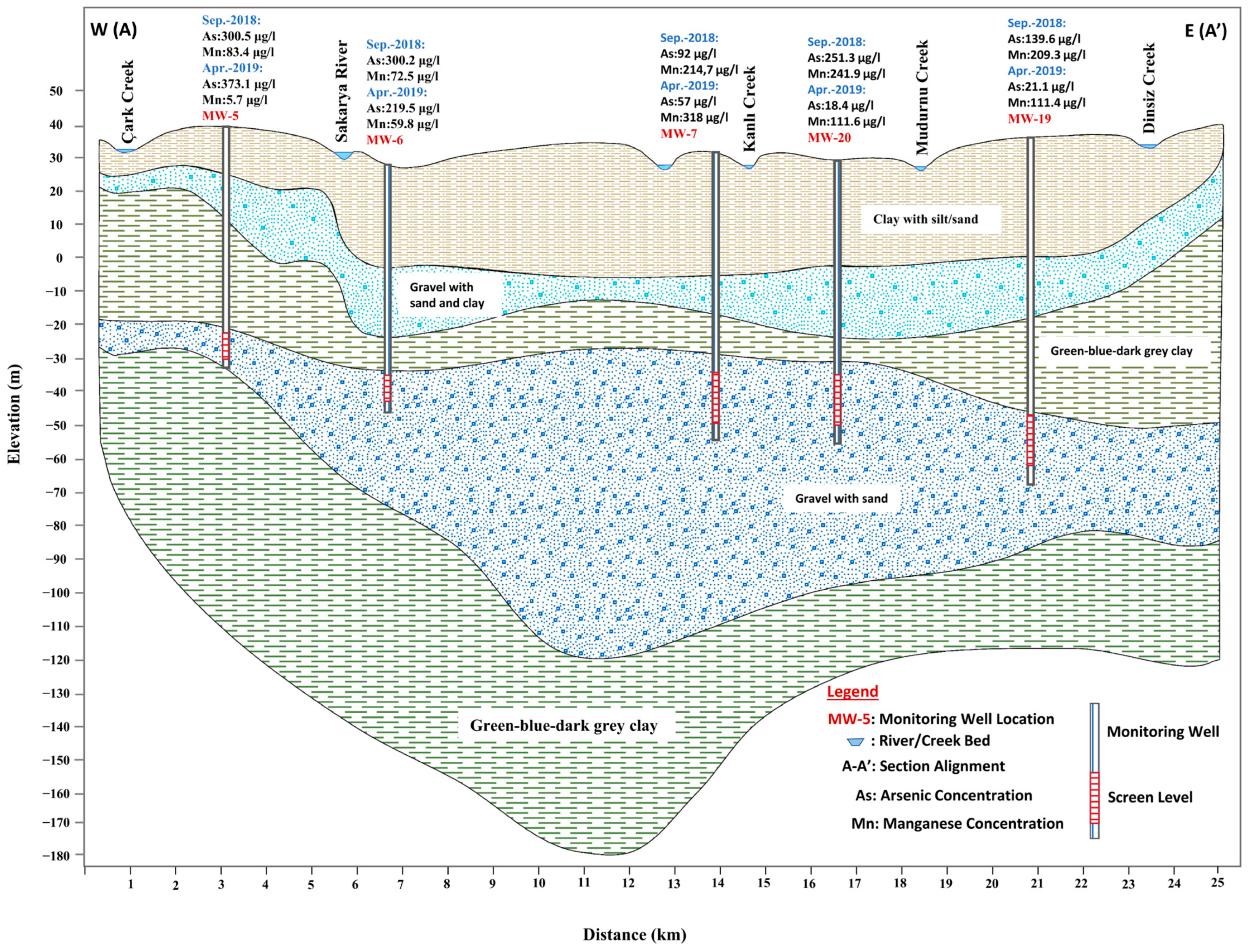
6.5. As and Mn Sources and Release Mechanism in Alluvium Aquifer

The mobilization and accumulation of arsenic in groundwater are significantly influenced by water–rock interactions in aquifers, which often provide favorable physical and geochemical conditions for these processes [1]. The identification of the primary sources of arsenic in a specific aquifer is a challenging process, given that multiple minerals can contribute to its release. Nevertheless, metal oxides, particularly iron and manganese oxides, are of great consequence in the cycling of arsenic within sedimentary aquifers, especially under reducing conditions [37,38,39]. Moreover, arsenic-related issues in younger sedimentary aquifers are frequently associated with strongly reducing environments.

The Lower Sakarya Basin is a low-lying delta characterized by a maximum slope of 5% and a geologically young alluvial aquifer formed of particles of weathered metamorphic, ophiolitic, and sedimentary rocks delivered by the Sakarya River from the southern region of the plain. The elevated concentrations of arsenic and manganese are closely associated with the geology and delta deposits of the Lower Sakarya Plain’s alluvial plain.

The locations of groundwater wells with arsenic and manganese concentrations above the permissible limits are spatially distributed in the middle of the plain like a belt as seen in Figure 6 and Figure 7. Upon examining the drill logs in proximity to these sites, the aquifer levels predominantly consist of medium to coarse grained limestone, schist, and serpentine pebbles, interlayered with substantial blue-green clay layers ranging from 25 to 102 m in thickness at intermediate depths. The dense blue-green clay layers (i.e., sign of reduced environment) and the slow recharge of deep alluvial aquifer, as indicated by low tritium concentrations, suggest that the oxygenation of the deep alluvial aquifer is slow. These conditions collectively facilitate the development and persistence of anoxic subsurface environments in the deep alluvial aquifer. On the western bank of the Sakarya River—particularly near Arifiye, the northeastern side of Sapanca Lake, and the northern downstream section of Mudurnu Creek—ancient marshlands are present. These areas are marked by limited aquifer recharge, as evidenced by borehole logs from the 1960s reporting [24] exceptionally low discharge rates ranging from 0.1 to 2 L/s. Methane generation has long been recognized as a persistent issue in this region. In 1965, Water Well No. 6653, drilled to a depth of 103.50 m, was immediately abandoned following a series of explosions during development. Similarly, in 2018, our field investigation documented those one of the two wells (No. 30339) nat the Adapazarı Meat Combine was decommissioned due to methane leakage and an ensuing explosion.

The oxidation of organic matter by microbial activity significantly depletes dissolved oxygen in soil and groundwater, resulting in a decrease in redox potential. As oxygen levels decline, manganese and iron oxides in sediments undergo reduction, releasing Mn(II) ions into the aqueous environment first, followed by Fe(II) ions under more strongly reducing conditions. The depletion of oxygen in groundwater systems is often exacerbated by increased organic carbon content and anthropogenic organic pollution. In the presence of Fe(II) ions, NO₃⁻ is typically absent, as nitrate reduction occurs under less reducing conditions. Conversely, when Mn is present, a partial reduction of NO₃⁻ may still occur. When sufficiently negative redox potential values are reached, SO₄²⁻ is reduced to H₂S and HS⁻, while organic substances are reduced to dissolved gases, specifically CO₂ and CH₄ [40].

Although classical redox sequences describe the stepwise reduction of nitrate, manganese, iron oxides, sulfate, and ultimately CO₂ to methane under increasingly reducing conditions, the geochemical conditions observed in this study suggest that varying degrees of redox conditions such as manganese/iron reduction, sulfate reduction, and methanogenesis developed locally within the deeper alluvial aquifer.

Despite the presence of ultramafic rocks fragments in deep alluvial aquifer sediments —which contribute significant amounts of iron—dissolved Fe concentrations in groundwater were below detection limits. This likely reflects the precipitation of Fe²⁺ as secondary iron sulfides (e.g., FeS or FeS₂), a common outcome under sulfate-reducing conditions. The absence of measurable Fe in groundwater does not preclude the occurrence of iron cycling, as Fe(III) oxides may still undergo reductive dissolution, releasing arsenic in the process. Therefore, even though Fe is not detected analytically, redox-mediated Fe–As interactions could also be controlling mechanism of arsenic mobility in the aquifer system. This is a well-known phenomenon in anoxic aquifers [1,41].

Similar geochemical conditions have been documented in urban coastal aquifer in Kocaeli, which lies to the west of Sapanca Lake and adjacent to the Lower Sakarya Basin. In this basin, Yolcubal et al. (2019) [19] reported the coexistence of elevated As and Mn concentrations in alluvial groundwater while Fe concentrations remained very low in water, and that the existence of Fe-Mn-reducing conditions in the alluvial sediments controlled the release of As into groundwater.

These geochemical signatures strongly suggest that intense reductive conditions, likely driven by the degradation of organic matter, are controlling arsenic and manganese mobilization in parts of the deep alluvial aquifer. This is particularly evident in well MW1, which was permanently closed due to methane accumulation and explosion risk. The well exhibited high concentrations of arsenic (161.70 µg/L), manganese (67.85 µg/L), and bicarbonate (556.11 mg/L), accompanied by very low levels of sulfate (0.20 mg/L) and nitrate (0.2–0.6 mg/L). These values are characteristic of a late-stage redox environment, where denitrification and sulfate reduction have likely been exhausted, and methanogenesis dominates. MW1 is located on the left bank of the Sakarya River, near marsh areas with high organic content, and is underlain by thick clay layers that restrict recharge and promote persistent anoxic conditions. Under such settings, arsenic can be released through the reductive dissolution of Mn and Fe oxides, and its mobility may be further enhanced by elevated pH and alkalinity. This case exemplifies how site-specific hydrogeological and geochemical conditions—including organic-rich zones, restricted flow, and redox stratification—can lead to localized arsenic enrichment in deep aquifer systems.

7. Conclusions

This study provides the first detailed overview of the hydrogeological, hydrogeochemical, and isotopic features of the Lower Sakarya River Basin. Groundwater samples from shallow (<60 m) and deep (>60 m) alluvial aquifers were carefully examined, allowing essential differences in recharge patterns, redox conditions, and trace element behaviors within this vital freshwater resource in northwestern Turkey to be clarified.

Significant natural contamination by arsenic and manganese, particularly in the deeper aquifer, was revealed by groundwater analyses. Elevated levels of arsenic (exceeding national drinking water standards in up to 41% of deep wells) and manganese (exceeding recommended limits in up to 44% of deep wells) highlight the influence of localized reducing conditions on contaminant mobility. Seasonal and depth-dependent redox gradients were observed, with arsenic and manganese enrichments concentrated in discrete zones where dissolved oxygen concentrations fell below 2 mg/L. These conditions coincide with low sulfate levels and very high bicarbonate concentrations, indicating active reduction pathways consistent with long-term anoxic evolution. In these zones, microbially driven degradation of organic matter depletes oxygen and promotes the reductive dissolution of manganese /iron oxyhydroxides, leading to the release of Mn(II) and the desorption or dissolution of arsenic into groundwater. These findings highlight the role of redox evolution in mobilizing trace elements under confined conditions, and that arsenic and manganese mobilization is primarily controlled by sediment chemistry and long-term redox evolution rather than recent recharge or anthropogenic activities. Serpentinite, schist, and other ophiolitic/metamorphic detritus transported by river processes into basin sediments were identified as the main natural sources of these contaminants.

In contrast, the shallow aquifer system—although affected by elevated nitrate, sulfate, and chloride levels from agricultural and domestic sources—exhibited consistently low arsenic concentrations below the maximum contaminant level. Seasonal redox fluctuations in the shallow zone influence manganese concentrations, but the aquifer’s more dynamic recharge regime and oxic conditions suppress widespread As mobilization.

Stable isotope analyses (δ¹⁸O, δ²H, and tritium) were employed to clarify recharge mechanisms, clearly distinguishing between the shallow aquifer’s rapid modern recharge and the deep aquifer’s slow, distant recharge. These hydrochemical and isotopic distinctions significantly influence contaminant distribution, mobility, and speciation within the aquifer system.

From a methodological perspective, the study demonstrates the value of combining field hydrochemistry with stable isotopes, tritium dating, mineralogical analysis, and statistical evaluation to delineate contaminant sources and mobilization pathways. The use of multiple lines of evidence allowed for a nuanced understanding of water–rock interaction, recharge processes, and geochemical evolution under varying redox regimes.

Future studies should include detailed vertical profiling of sediments, groundwater, and arsenic and manganese speciation. These would further elucidate the mechanisms governing contaminant release, migration, and attenuation across space and time. Additionally, the delineation of vertical and lateral connectivity between aquifer units would support the design of sustainable abstraction and protection strategies in this strategic freshwater basin.

References

1. Smedley, P.L.; Kinniburgh, D.G. A review of the source, behavior and distribution of arsenic in natural waters. Appl. Geochem. 2002, 17, 517–568. [Google Scholar] [CrossRef]
2. Muzaffar, S.; Khan, J.; Srivastava, R.; Gorbatyuk, M.S.; Athar, M. Mechanistic understanding of the toxic effects of arsenic and warfare arsenicals on human health and environment. Cell Biol. Toxicol. 2023, 39, 85–110. [Google Scholar] [CrossRef]
3. UNICEF; World Health Organization. Arsenic Primer: Guidance on the Investigation and Mitigation of Arsenic contamination; UNICEF: New York, NY, USA, 2018. [Google Scholar]
4. Akter, K.F.; Chen, Z.; Smith, L.; Davey, D.; Naidu, R. Speciation of arsenic in ground water samples: A comparative study of CE-UV, HG-AAS and LC-ICP-MS. Talanta 2005, 68, 406–415. [Google Scholar] [CrossRef]
5. Apello, T. Arsenic in Groundwater: A World Problem; Netherlands National Committee for the IAH: Utrecht, The Netherlands, 2008; Volume 5. [Google Scholar]
6. Shaji, E.; Santosh, M.; Sarath, K.V.; Prakash, P.; Deepchand, V.; Divya, B.V. Arsenic contamination of groundwater: A global synopsis with focus on the Indian Peninsula. Geosci. Front. 2021, 12, 101079. [Google Scholar] [CrossRef]
7. Sadiq, M. Arsenic chemistry in soils: An overview of thermodynamic predictions and field observations. Water Air Soil. Pollut. 1997, 93, 117–136. [Google Scholar] [CrossRef]
8. Podgorski, J.; Berg, M. Global threat of arsenic in groundwater. Science 2020, 368, 845–850. [Google Scholar] [CrossRef]
9. Bhattacharya, P.; Chatterjee, D.; Jacks, G. Occurrence of arsenic-contaminated groundwater in alluvial aquifers from delta plains, eastern India: Options for safe drinking water supply. Int. J. Water Resour. Dev. 1997, 13, 79–92. [Google Scholar] [CrossRef]
10. Harvey, C.F.; Swartz, C.H.; Badruzzaman, A.B.M.; Keon-Blute, N.; Yu, W.; Ali, M.A.; Jay, J.; Beckie, R.; Niedan, V.; Brabander, D. Arsenic mobility and groundwater extraction in Bangladesh. Science 2002, 298, 1602–1606. [Google Scholar] [CrossRef]
11. Polizzotto, M.L.; Harvey, C.F.; Li, G.; Badruzzman, B.; Ali, A.; Newville, M.; Sutton, S.; Fendorf, S. Solid-phases and desorption processes of arsenic within Bangladesh sediments. Chem. Geol. 2006, 228, 97–111. [Google Scholar] [CrossRef]
12. Yadav, M.K.; Saidulu, D.; Gupta, A.K.; Ghosal, P.S.; Mukherjee, A. Status and management of arsenic pollution in groundwater: A comprehensive appraisal of recent global scenario, human health impacts, sustainable field-scale treatment technologies. J. Environ. Chem. Eng. 2021, 9, 105203. [Google Scholar] [CrossRef]
13. Zahid, A.; Hassan, M.Q.; Breit, G.N.; Balke, K.D.; Flegr, M. Accumulation of iron and arsenic in the Chandina alluvium of the lower delta plain, Southeastern Bangladesh. Environ. Geochem. Health 2009, 31 (Suppl. S1), S69–S84. [Google Scholar] [CrossRef]
14. Akbulut, N.E.; Tuncer, A.M. Accumulation of heavy metals with water quality parameters in Kızılırmak River Basin (Delice River) in Turkey. Environ. Monit. Assess. 2010, 173, 387–395. [Google Scholar] [CrossRef]
15. Alptekin, C.; Yuce, G. Observation of excess heavy metal concentrations in water resources to infer surface water influences on shallow groundwater: A typical example of the Porsuk River (Eskisehir-Turkey). Water Resour. 2016, 43, 184–199. [Google Scholar] [CrossRef]
16. Davraz, A.; Batur, B. Hydrogeochemistry characteristics of groundwater and health risk assessment in Yalvaç–Gelendost basin (Turkey). Appl. Water Sci. 2021, 11, 67. [Google Scholar] [CrossRef]
17. Küçüksümbül, A.; Akar, A.T.; Tarcan, G. Source, degree and potential health risk of metal(loid)s contamination on the water and soil in the Söke Basin, Western Anatolia, Turkey. Environ. Monit. Assess. 2021, 194, 6. [Google Scholar] [CrossRef]
18. Simsek, C. Assessment of naturally occurring arsenic contamination in the groundwater of Sarkisla Plain (Sivas/Turkey). Environ. Earth Sci. 2012, 68, 691–702. [Google Scholar] [CrossRef]
19. Yolcubal, İ.; Ataş Gündüz, Ö.C.; Kurtuluş, N. Origin of salinization and pollution sources and geochemical processes in urban coastal aquifer (Kocaeli, NW Turkey). Environ. Earth Sci. 2019, 78, 181. [Google Scholar] [CrossRef]
20. Baba, A.; Sözbilir, H. Source of arsenic based on geological and hydrogeochemical properties of geothermal systems in Western Turkey. Chem. Geol. 2012, 334, 364–377. [Google Scholar] [CrossRef]
21. Ravenscroft, P.; Brammer, H.; Richards, K. Arsenic Pollution: A Global Synthesis; Wiley: Hoboken, NJ, USA, 2009. [Google Scholar] [CrossRef]
22. Gedik, İ.; Aksay, A. 1:100,000 Scale Geological Maps of Turkey, No. 32, Adapazarı-G25 Sheet; General Directorate of Mineral Research and Exploration (MTA): Ankara, Turkey, 2002. [Google Scholar]
23. Timur, E.; Aksay, A. 1:100,000 Scale Geological Maps of Turkey, No. 31, Adapazarı-G24 Sheet; General Directorate of Mineral Research and Exploration (MTA): Ankara, Turkey, 2002. [Google Scholar]
24. Okay, H.; Boydaș, T.; Giritlioğlu, T. Lower Sakarya Basin Groundwater Reserve Report; Republic of Turkey Ministry of Energy and Natural Resources, General Directorate of State Hydraulic Works, Department of Groundwater: Ankara, Turkey, 1966. [Google Scholar]
25. Sarı, İ.; Kurt, M. Prospection Report of Iron and Manganese Based Metallic Mines of Adapazarı-Sapanca-Geyve-Akyazı Surroundings; General Directorate of Mineral Research and Exploration: Ankara, Turkey, 1983. [Google Scholar]
26. Wijkerslooth, P. Manganese Prospection Between Bilecik and Adapazarı (MTA Compilation Report No: 1143); General Directorate of Mineral Research and Exploration (MTA): Ankara, Turkey, 1939. [Google Scholar]
27. APHA Method 2320; Standard Methods for the Examination of Water and Wastewater. American Public Health Association: Washington, DC, USA, 2005.
28. Ramachandran, M.; Schwabe, K.A.; Ying, S.C. Shallow Groundwater Manganese Merits Deeper Consideration. Environ. Sci. Technol. 2021, 55, 3465–3466. [Google Scholar] [CrossRef]
29. Ollivier, P.; Surdyk, N.; Azaroual, M.; Besnard, K.; Casanova, J.; Rampnoux, N. Linking water quality changes to geochemical processes occurring in a reactive soil column during treated wastewater infiltration using a large-scale pilot experiment: Insights into Mn behavior. Chem. Geol. 2013, 356, 109–125. [Google Scholar] [CrossRef]
30. Appelo, C.A.J.; Van Der Weiden, M.J.J.; Tournassat, C.; Charlet, L. Surface complexation of ferrous iron and carbonate on ferrihydrite and the mobilization of arsenic. Environ. Sci. Technol. 2002, 36, 3096–3103. [Google Scholar] [CrossRef]
31. Ekmekçi, M.; Gültekin, F. Evaluation of Environmental Stable Isotope Content of Eastern Black Sea Section Waters; National Engineering Geology Symposium: Trabzon, Turkey, 2015; pp. 459–466. [Google Scholar]
32. Eisenlohr, T.; Pfister, M.; Balderer, W. Environmental isotope study and 2-D modelling of cold and thermal karst within the Gemlik (Bursa) area of Northwestern Turkey. In Karst Waters & Environmental Impacts; Günay, G., Johnson, A.I., Eds.; Balkema: Rotterdam, The Netherlands, 1997; ISBN 90-5410-656-4. [Google Scholar]
33. Craig, H. Isotopic variations in meteoric waters. Science 1961, 133, 1702–1703. [Google Scholar] [CrossRef]
34. Boyle, R.W.; Jonasson, I.R. The geochemistry of arsenic and its use as an indicator element in geochemical prospecting. J. Geochem. Explor. 1973, 2, 251–296. [Google Scholar] [CrossRef]
35. Pokrovski, G.S.; Sanchez-Valle, C.; Guillot, S.; Borisova, A.Y.; Muñoz, M.; Auzende, A.-L.; Proux, O.; Roux, J.; Hazemann, J.-L.; Testemale, D.; et al. Redox dynamics of subduction revealed by arsenic in serpentinite. Geochem. Perspect. Lett. 2022, 22, 36–41. [Google Scholar] [CrossRef]
36. Faust, G.T. The hydrous nickel-magnesium silicates-the garnierite group. Am. Mineral. J. Earth Planet. Mater. 1966, 51, 279–298. [Google Scholar]
37. Deuel, L.E.; Swoboda, A.R. Arsenic Solubility in a Reduced Environment. Soil. Sci. Soc. Am. J. 1972, 36, 276–278. [Google Scholar] [CrossRef]
38. De Vitre, R.; Belzile, N.; Tessier, A. Speciation and adsorption of arsenic on diagenetic iron oxyhydroxides. Limnol. Oceanogr. 1991, 36, 1480–1485. [Google Scholar] [CrossRef]
39. Widerlund, A.; Ingri, J. Early diagenesis of arsenic in sediments of the Kalix River estuary, northern Sweden. Chem. Geol. 1995, 125, 185–196. [Google Scholar] [CrossRef]
40. Golterman, H.; Stumm, W.; Morgan, J.J. Aquatic Chemistry. An Introduction Emphasizing Chemical Equilibria in Natural Waters. J. Ecol. 1982, 70, 924–925. [Google Scholar] [CrossRef]
41. Postma, D.; Larsen, F.; Thai, N.T.; Trang, P.T.K.; Jakobsen, R.; Nhan, P.Q.; Long, T.V.; Viet, P.H.; Murray, A.S. Groundwater arsenic concentrations in Vietnam controlled by sediment age. Nat. Geosci. 2012, 5, 656–661. [Google Scholar] [CrossRef]
Figure 1. Geological map of the study area (modified after Gedik and Aksay, 2002; Timur and Aksay, 2002 [22,23]).
Water 17 01931 g001
Figure 2. Subsurface geological cross-section of the alluvial plain. The cross-section line is indicated in Figure 1 As and Mn concentrations measured at sample wells are also depicted in the cross-section.
Water 17 01931 g002
Figure 3. Map depicting contours of the groundwater potentiometric surface. The map also indicates the locations of groundwater samplings and well core samples.
Water 17 01931 g003
Figure 4. Piper diagram of groundwater in the alluvium aquifer for dry and wet seasons.
Water 17 01931 g004
Figure 5. Dot distribution of NO3 concentrations in shallow and deep alluvium aquifers in both dry and wet seasons.
Water 17 01931 g005
Figure 10. XRD diffractogram of Alancuma composite core samples obtained from depths of (a) 0–50 m, (b) 50–110 m.
Water 17 01931 g010
Disclaimer/Publisher’s Note: The statements, opinions and data contained in all publications are solely those of the individual author(s) and contributor(s) and not of MDPI and/or the editor(s). MDPI and/or the editor(s) disclaim responsibility for any injury to people or property resulting from any ideas, methods, instructions or products referred to in the content.