Long-Term Monitoring of Surface Water Dynamics and Analysis of Its Driving Mechanism: A Case Study of the Yangtze River Basin

Abstract

In-depth insights into the profound impacts of climate change and human activities on water resources are garnered through the dynamic changes in surface water, a crucial aspect of effective water resource management and the preservation of aquatic ecosystems. This paper introduces an innovative approach employing the random forest algorithm for the systematic extraction and monitoring of surface water at large regional or national scales. This method integrates spectral bands, spectral indices, and digital elevation model data, offering a novel perspective on this critical task. A data-filling model is proposed to mitigate the impact of missing data due to cloud cover. Leveraging the capabilities of the Google Earth Engine (GEE), detailed information on surface water dynamics during the rainy and dry seasons in the Yangtze River Basin (YRB) from 1991 to 2021 is extracted using Landsat time series imagery. The analysis encompasses spatial-temporal variation characteristics and trends, with a specific focus on the intricate interplay between the areal extent of surface water and hydro-meteorological factors in each sub-basin of the YRB. Importantly, this includes considerations of potential groundwater contributions to surface water. Key findings from our research include: (1) Achieving a remarkable overall classification accuracy of 0.96 ± 0.03 in obtaining reliable surface water datasets with the support of GEE. (2) Identifying significant trends, such as a noteworthy increase in rainy season surface water bodies (+248.0 km²·yr⁻¹) and a concerning decrease in surface ice/snow cover during both rainy and dry seasons, with change rates of −39.7 km²·yr⁻¹ and −651.3 km²·yr⁻¹, respectively. (3) Uncovering the driving mechanisms behind these changes, revealing positive correlations between the areal extent of rainy season surface water bodies and precipitation, as well as negative correlations between surface ice/snow cover area and average surface skin temperature. It is crucial to note that these driving factors exhibit variation among secondary river systems, underscoring the complexity of surface water dynamics. Furthermore, comparative analyses with existing surface water products are conducted, contributing to a deeper understanding of the advantages and uncertainties inherent in our proposed extraction method. The proposed method for large-scale surface water extraction not only enhances the monitoring of spatio-temporal surface water dynamics in the YRB but also provides valuable insights for the sustainable utilization and protection of water resources, considering the potential role of groundwater in supplementing surface water.

1. Introduction

Water resources are an indispensable basic condition for human survival and an irreplaceable basic natural and strategic resource to maintain the function of Earth’s ecological system and support the development of social and economic systems [1]. With the acceleration of urbanization [2] and sharp increase in the world’s human population [3], the deterioration of the ecological environment, the serious waste of industrial and domestic water, and the irrational utilization of water resources have led to a reduction in available water resources, forcing the world’s water resources to become increasingly scarce [4]. Climate change affects global temperature and rainfall patterns which, in turn, affect the intensity and frequency of extreme weather events and reflect an increasing instability of precipitation, storms, floods, droughts, and ice/snow disasters [5]. Surface water is a general term for dynamic and static water on the land surface, also known as ‘land water’, which includes all kinds of liquid and solid water bodies (e.g., rivers, lakes, swamps and glaciers). As the main component of water resources in various countries, surface water is not only a key component of the hydrological cycle but also an important source of water for human production and life [6]. Extracting and monitoring surface water can provide a scientific basis for water resource management and utilization. The dynamic changes in surface water may cause some disasters (e.g., floods and droughts), and continuous monitoring of surface water dynamics can help alert potential disaster risks and reduce their impact on human society and the natural environment. Therefore, systematic monitoring of surface water is of great significance for the optimal allocation of water resources, the coordination of the relationship between the ecological environment and economic development, and the achievement of sustainable development goals.

The launch of the first Earth observation satellite (i.e., the Earth Resources Technology Satellite, later renamed Landsat-1) triggered a global revolution in remote sensing science and technology that continues until today [7]. In the ensuing decades, a variety of satellite sensors have been developed and used to detect and extract land surface features and monitor land use changes on Earth’s surface [8,9,10,11,12]. As a key theme of Earth observation, the surface water extent dynamics extracted from satellite imagery have been widely used for hydrological monitoring, surface water change detection, and drought and flood prediction [13,14,15]. Data accessibility, availability and resolution are essential considerations in selecting appropriate satellite imagery for monitoring surface water dynamics. The Landsat series of satellites for moderate-resolution optical remote sensing (30 m) have been observing Earth for 50 years, providing the longest continuous record of Earth’s land surfaces. In particular, the United States Geological Survey announced its Landsat Date Distribution policy in 2008 that made the entire Landsat archive freely available to the public, making it possible to monitor long-term surface water dynamics, as well as changes in other land cover types, at regional, national and global scales [16,17,18,19,20].

With the development of remote sensing technology, many methods for surface water extraction have been proposed. The principle of extracting surface water is that the reflectance of water in the near-infrared (NIR) and shortwave infrared (SWIR) bands is clearly lower than that of other land cover types. On this basis, more effective water indices have been proposed to highlight surface water, such as normalized difference water index (NDWI) [21], modified NDWI (MNDWI) [22], and normalized difference snow index (NDSI) [23,24]. A simple and efficient approach for surface water extraction is to use these indices to set the optimal threshold value for binary classification. Several studies have combined different indices to distinguish water from non-water, especially the combination of normalized difference vegetation index (NDVI) [25] and MNDWI, which has shown its feasibility of extracting surface water [26]. However, the identification of threshold values might result in under- or over-estimation of surface water extent. In addition, the phenomenon of homospectral foreign matters caused by ground objects with similar spectral reflection characteristics to surface water (e.g., cloud/cloud shadows) would further lead to misclassification. At present, the commonly used methods of extracting surface water are to generate land cover maps using different classifiers to extract surface water, such as spectral-based supervised classification (e.g., support vector machines [27]), decision tree classification based on expert knowledge [28], object-oriented image classification [29] and deep learning image classification (e.g., convolutional neural networks [30]). Recently, cloud computing has enabled researchers to access and analyze massive amounts of remote sensing image data in the cloud without the need to download image data to a local computer. Powered by the Google Cloud Platform, the GEE [31] provides free access to massive amounts of Earth science data (e.g., satellite imagery, weather and climate data) as well as algorithms that enable developers to perform geospatial processing at large regional, national and global scales [32,33,34]. As a supervised learning algorithm, random forest (RF) [35] used the limited multispectral bands as inputs for classification in previous studies, which had not been fully exploited. With the powerful GEE computing platform, multidimensional data can be introduced into the RF model to further improve its classification performance for the long-term monitoring of surface water dynamics at scale.

As the third largest river in the world and the largest river in China, the Yangtze River secures the country’s water and food supply with its vast river and lake water systems, which plays an important role in the country’s economic and social development [36,37]. With the development of the Yangtze River Economic Belt and the integrated development of the Yangtze River Delta rising to the national strategies [38,39], the YRB has become the focus and vitality of China’s economy. However, lake shrinkage and the degradation of wetland ecosystem function in the middle and lower reaches of the Yangtze River are increasingly prominent as a result of unreasonable development and utilization [40]. Extreme weather events caused by climate change have also aggravated flood and drought disasters that seriously affect economic development and threaten residents’ lives and safety. River flows, lake levels and ice/snow cover show obvious seasonal changes, reflected in seasonal variations in surface water area. However, many studies have focused on the annual dynamics of single surface water bodies or ice/snow cover, with relatively few exploring surface water bodies and ice/snow cover simultaneously. The detailed dynamic characteristics of surface water (i.e., surface water bodies and ice/snow cover) in the rainy and dry seasons are ignored despite their importance in guiding surface water management, flood control and drought relief, and early warning of ice/snow disasters. Therefore, while strengthening the protection and restoration of the aquatic ecological environment, it is particularly important to accurately monitor and systematically analyze the long-term dynamics of surface water in the YRB during the rainy and dry seasons.

Supported by the GEE, this paper looks into the following aspects related to the extraction of surface water, detection of surface water change, and the analysis of the driving factors affecting dynamic changes in surface water. The specific objectives of this study are to (1) propose a method for accurately extracting and monitoring surface water at large regional or national scales; (2) apply the proposed method to the analysis of the spatiotemporal characteristics and dynamics of rainy and dry season surface water in the YRB from 1991 to 2021; (3) explore the driving mechanisms of surface water change related to hydro-meteorological elements and human activities.

2. Materials and Methods

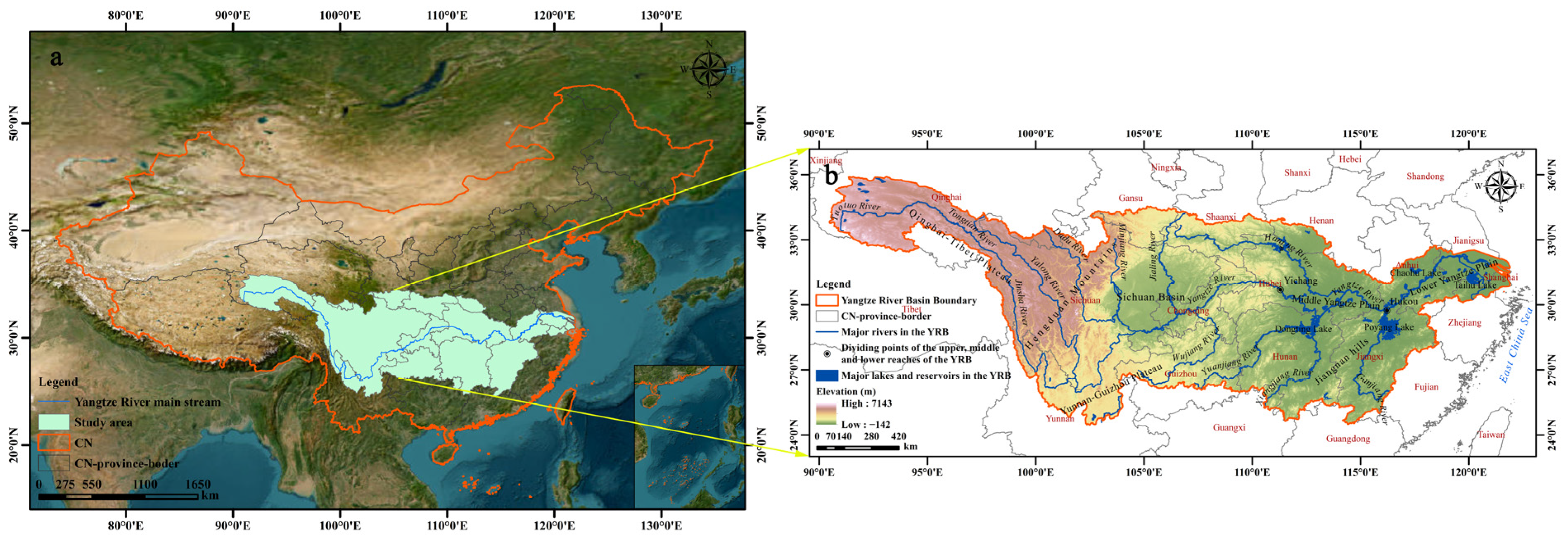
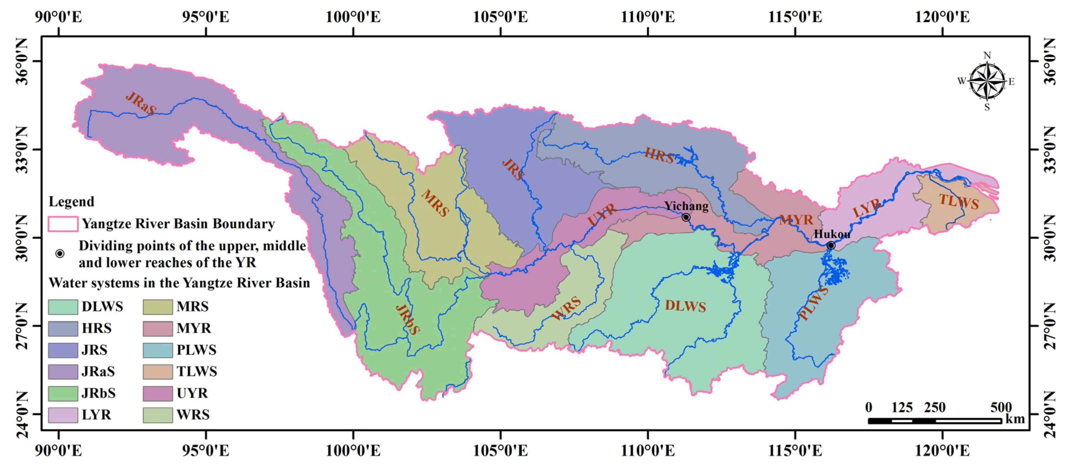
2.1. Study Area

As the third largest river basin in the world, the YRB consists of the vast area through which the mainstream and tributaries of the Yangtze River flow (90°33′ E–122°25′ E, 24°30′ N–35°45′ N). The Yangtze River has a total length of more than 6300 km and covers an area of 1.8 million km², accounting for 18.8% of China’s total land area (Figure 1). The upper, middle and lower reaches of the Yangtze River are demarcated by the cities of Yichang and Hukou. The upstream tributaries include the Yalong River, Minjiang River, Jialing River and Wujiang River. The middle and lower reaches of the Yangtze River run through hills and plains at lower altitudes. The main tributaries include the Han River, Xiangjiang River, Yuanjiang River and Ganjiang River. The middle and lower reaches of the Yangtze River contain the most concentrated distribution of freshwater lakes in China. Four of the five largest freshwater bodies in China belong to the YRB, namely Poyang Lake, Dongting Lake, Taihu Lake and Chaohu Lake. Among them, Poyang Lake is the largest freshwater lake in China. The terrain of the YRB is high in the west and low in the east, presenting a three-level stepped terrain. The river flows through the Qinghai–Tibet Plateau, Hengduan Mountains, Yunnan–Guizhou Plateau, Sichuan Basin, Jiangnan hills, and plains in its middle and lower reaches, and finally flows into the East China Sea. Most of the basin is located in the subtropical monsoon climate zone, which is warm and humid, with an average annual precipitation of 1067 mm.

Annual precipitation and temperature in the YRB from 1981 to 2021 are shown in Figure S1, with an average annual precipitation of 1110.5 mm. Affected by the monsoon climate, inter-annual variation in precipitation is obvious. The illustration in Figure S1 shows the average monthly precipitation and monthly mean air temperature. Precipitation is unevenly distributed throughout the year; in the rainy season (May–October) it accounts for more than 70% of annual precipitation. Raw meteorological data were obtained from the Climate Hazards Group Infrared Precipitation with Station data (CHIRPS) [41] and ERA5-Land [42] datasets. The Changjiang Water Resources Commission (CWRC) divides the YRB into 12 water systems, namely five main river systems, three north bank water systems and four south bank water systems (Figure 2).

2.2. Datasets

Landsat satellites have been consistently gathering image data about the Earth’s land surface since 1972. To systematically analyze the dynamics of surface water in the study area during the period 1991–2021, Landsat series of imagery were used to map surface water. Specific data were Landsat 5 Thematic Mapper (TM) Collection 1 Tier 1 calibrated top-of-atmosphere (TOA) reflectance [43], Landsat 7 Collection 1 Tier 1 and Real-Time data calibrated TOA reflectance, and Landsat 8 Collection 1 Tier 1 and Real-Time data calibrated TOA reflectance. Tier 1 refers to data that meet geometric and radiometric quality requirements. Figure 3 shows the distribution of the total number of observations per pixel for the study area during the rainy season from 1991 to 2021 and the distribution of the total number of dry season observations is presented in Figure S2.

To improve the classification accuracy, spectral indices such as NDWI, MNDWI, NDVI, normalized difference built-up index (NDBI) [44] and normalized difference moisture index (NDMI) [45,46] were calculated and added as bands to each scene of the image collections. In addition, from the perspective of altitude, the Shuttle Radar Topography Mission (SRTM) digital elevation dataset Version 4 [47] was added to the Landsat images in the image collections to improve recognition accuracy. To establish highly reliable sample data, the Global Land Ice Measurements from Space (GLIMS) Current dataset provided by the National Snow and Ice Data Center [48,49], together with the Joint Research Centre (JRC) Yearly Water Classification History dataset [20] were utilized as auxiliary data to revalidate the samples that had been visually interpreted pixel by pixel. To analyze the impact of climate change and human activities on land surface water, hydro-meteorological data and relevant regional statistics were collected. The climate data included precipitation, temperature (including surface skin temperature and surface air temperature) and evaporation, which were derived from the CHIRPS, ERA5-Land and TerraClimate [50] datasets, respectively. In addition, hydrologic data for surface runoff were extracted from the Famine Early Warning Systems Network (FEWS NET) Land Data Assimilation System (FLDAS) [51] dataset. All these data were available in the Earth Engine Data Catalog and could be imported into a personal script environment for geospatial analysis. It should be noted that meteorological and hydrological datasets are mostly monthly, daily or hourly data, which may require unit conversion or conversion to data within the time range required for the study, according to the data description.

2.3. Methodology

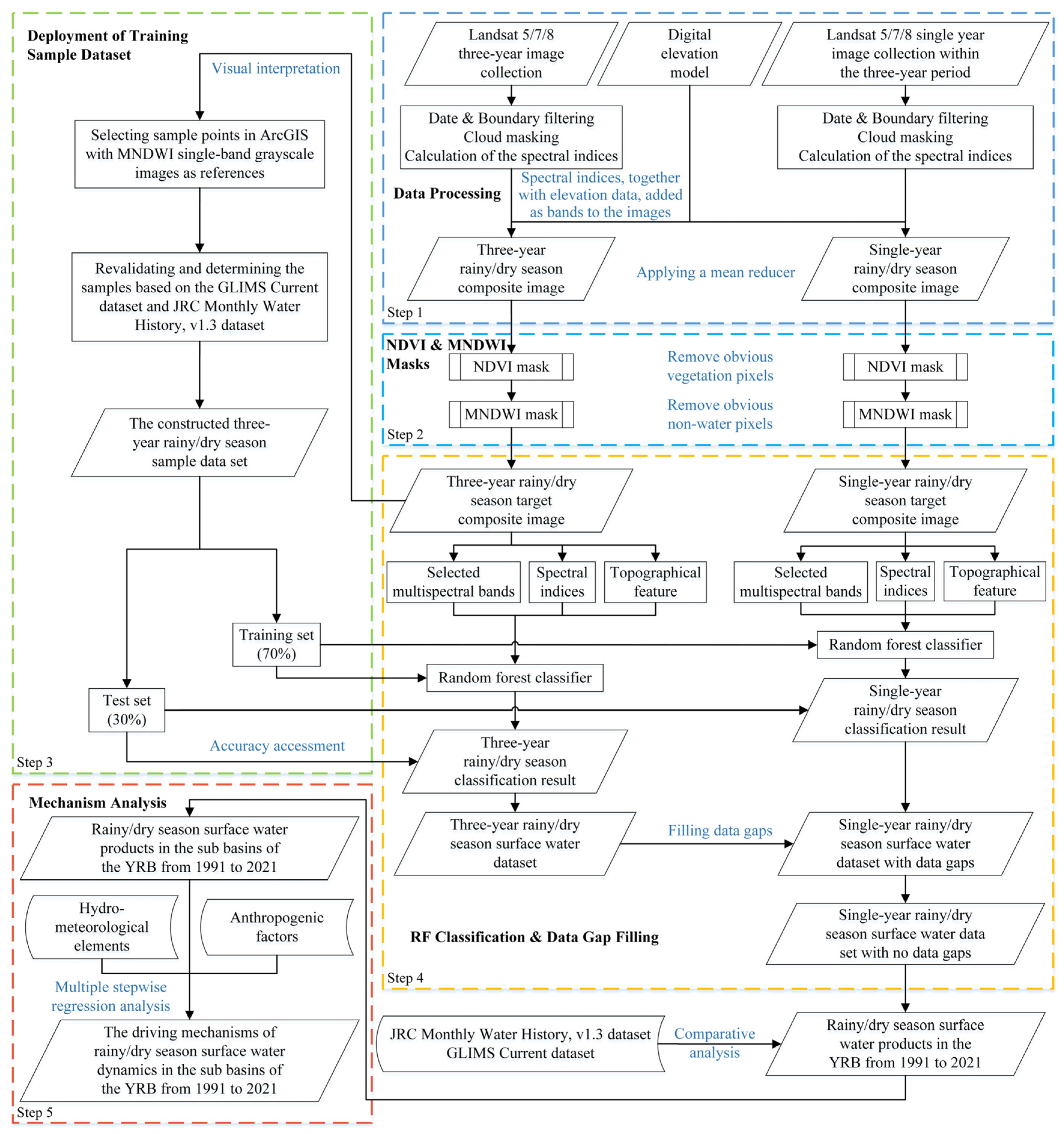
2.3.1. Technical Process

The overall technical process was comprised of five steps, as illustrated in Figure 4.

• The required image collections were obtained by limiting the date range and the study area boundary. Cloud masking was then applied to each scene of the image collections. Spectral indices and elevation data were added as bands to each image in the image collections. The cloud-free composite images in the rainy and dry seasons were obtained by applying a mean reducer to the integrated image collections.
• To improve the efficiency and accuracy of surface water extraction, NDVI and MNDWI masks were used to remove obvious vegetation and non-water pixels.
• With MNDWI single-band grayscale images as references, sample points were first selected by visual interpretation. By comparison with the GLIMS Current dataset and JRC Monthly Water History Version 1.3 dataset, the samples were revalidated and determined according to the principles of “complete consistency” and “temporal stability” of land type attributes [52].
• To further extract surface water, the RF model was applied for classification. Meanwhile, an approach was proposed to fill data gaps that existed in single-year rainy and dry season composite images. The rainy and dry season composite images from 1991 to 2021 were classified year by year to monitor the spatial and temporal changes in surface water extent in the YRB.
• Based on the hydro-meteorological factors, multiple stepwise regression modeling was applied to quantitatively analyze the impact of climate change on surface water dynamics. Factors that might affect the distribution of surface water due to human activities (e.g., inter-basin water diversion projects and artificial control of surface water distribution using water conservancy facilities) were qualitatively discussed.

2.3.2. Data Processing

Affected by the uneven distribution of precipitation within a year, the surface water in the YRB presents obvious seasonal differences. To obtain abundant surface water information, based on the Landsat 5/7/8 Collection 1 Tier 1 TOA Reflectance products, Landsat time series datasets for the rainy and dry seasons (from November to April of the following year) of the YRB, rather than the whole year were generated by limiting the dates and study area. Here, Landsat 5 and Landsat 8 image data were mainly selected, and Landsat 7 image data were only used when the data were alternated to minimize the impact of data gaps since 2003, caused by a scan line corrector (SLC) failure. Cloud masking was then applied to each individual image of the obtained image collections by using the built-in cloud scoring algorithm “simpleCloudScore”, and pixels with a cloud score higher than 90 were masked out. Spectral indices (NDWI, MNDWI, NDVI, NDBI and NDMI) were calculated for each scene in the image collections, and these indices together with the digital elevation model (DEM) data were added as bands to the images in the image collections. Rainy and dry season cloud-free composite images for the YRB from 1991 to 2021 were obtained by applying a mean reducer to the integrated image collections. The spectral indices involved are defined as follows:

$$\mathrm{NDWI}=\frac{{\rho }_{Green}-{\rho }_{NIR}}{{\rho }_{Green}+{\rho }_{NIR}},$$

(1)

$$\mathrm{MNDWI}=\frac{{\rho }_{Green}-{\rho }_{SWIR1}}{{\rho }_{Green}+{\rho }_{SWIR1}},$$

(2)

$$\mathrm{NDVI}=\frac{{\rho }_{NIR}-{\rho }_{\mathrm{Re}d}}{{\rho }_{NIR}+{\rho }_{\mathrm{Re}d}},$$

(3)

$$\mathrm{NDBI}=\frac{{\rho }_{SWIR1}-{\rho }_{NIR}}{{\rho }_{SWIR1}+{\rho }_{NIR}},$$

(4)

$$\mathrm{NDMI}=\frac{{\rho }_{NIR}-{\rho }_{SWIR1}}{{\rho }_{NIR}+{\rho }_{SWIR1}},$$

(5)

where ${\rho }_{Green}$, ${\rho }_{NIR}$, ${\rho }_{SWIR1}$, and ${\rho }_{\mathrm{Re}d}$ represent the reflectance values of the green band, near-infrared band, shortwave infrared band 1, and red band in Landsat images, respectively.

2.3.3. An Approach to Filling Data Gaps

Landsat 5/7/8 visits the same spot on Earth every 16 days, which means approximately 12 images containing this spot are taken over a six-month period (and more where the scenes overlap). However, given the conditions that can affect satellite imaging, such as “plum rain”, prolonged cloud cover in high-altitude mountainous areas, unexpected bad weather and sensor problems, these circumstances would affect the image acquisition, resulting in poor image quality, as presented in Figure 3 and Figure S2. Moreover, according to the World Reference System-2 (WRS-2), more than 100 Landsat scenes are required to cover the entire YRB, presenting additional complications. The World Reference System is a global system that catalogs Landsat data by Path and Row number, and Landsat 5, 7 and 8 follow WRS-2. Therefore, it is not surprising to see data gaps in the composite images during the rainy and dry seasons after executing the data processing procedure in Section 2.3.2. To deal with these data gaps, an approach was proposed that involved constructing a three-year period of image datasets. The specific steps were as follows:

• Since a single year’s rainy/dry season cloud-free composite images had data gaps, we extended the data by constructing a three-year period of image datasets (the previous year, the focal year, and the following year) during the rainy/dry seasons. The three-year period of cloud-free rainy/dry season composite images without data gaps were then obtained by executing the data processing procedure in Section 2.3.2;
• The RF algorithm was applied to the obtained composite images (including the three-year period of rainy/dry season composite images and the rainy/dry season composite images of any year within the three-year period) for classification to extract surface water. The data gaps that existed in a single year’s rainy/dry season composite images were filled using the extracted three-year period of rainy/dry season surface water, thus obtaining the single year’s rainy/dry season surface water without data gaps.

2.3.4. Removing Obvious Non-Water Pixels with NDVI and MNDWI Masks

Surface water has lower NDVI and higher MNDWI values than other land cover types. To improve the efficiency and accuracy of surface water extraction, NDVI and MNDWI masks were used to remove pixels with high NDVI values or low MNDWI values. Thresholds were identified through repeated comparison experiments. For rainy season composite images, the threshold value for NDVI was set to 0.3, and that for MNDWI was set to −0.25. Pixels with NDVI values greater than or equal to 0.3 and MNDWI values less than −0.25 were masked out using the “updateMask()” function. Similarly, for the dry season composite images, the threshold value was set to 0.25 for NDVI and −0.2 for MNDWI. The threshold range could be adjusted appropriately according to the spectral characteristics of the composite images. This procedure not only removed obvious vegetation and non-water pixels but also saved time and reduced labor costs for the subsequent construction of training sample datasets and extraction of surface water.

2.3.5. Deployment of Sample Datasets

The construction of sample datasets was based on the three years of rainy/dry season composite images obtained after executing step 2. In view of the fact that many of the existing land cover products are annual classification results, and there are obvious temporal differences from our research data, it is not appropriate to obtain samples from existing annual land cover products or land cover products with lower resolution. Besides, selecting samples from annual land cover products might lead to sample bias because of the lack of samples of seasonal land cover change. In this study, sample points were selected through manual visual interpretation with MNDWI single-band grayscale images as references. To facilitate the deployment of sample points, the image data obtained in Section 2.3.4 were exported to Google Cloud Storage and then downloaded to a local computer. The whole process of deployment of samples was conducted in ArcGIS 10.6 and QGIS 3.10. Here, the GLIMS Current dataset and JRC Monthly Water History Version 1.3 dataset were used as validation data, the sample points were revalidated and determined. The land cover types in the study area were divided into three categories: (1) water bodies, including rivers, lakes, reservoirs, ponds and wetlands; (2) ice/snow; (3) non-water, which was mainly cropland, woodland, grassland, built-up land and bare land. Sample datasets in the rainy and dry seasons were deployed separately within every three-year period from 1991 to 2021, which was consistent with the constructed three-year period of rainy and dry season composite images. A total of 22 sample datasets were deployed, each containing nearly 5000 samples. To effectively distinguish between surface water and other surface features, false color composites of TM bands 4 (NIR), 5 (SWIR1) and 3 (red) for Landsat 4/5, and Operational Land Imager (OLI) bands 5 (NIR), 6 (SWIR1) and 4 (red) for Landsat 8 were generated. This band combination showed land in shades of orange and green; ice/snow in very bright rose reds and water bodies in shades of blue. Figure 5 shows the deployment of sample points in the YRB during the rainy seasons from 2003 to 2005, according to the three-year rainy season composite image from 2003 to 2005. This constructed sample dataset could be used for the classification of the rainy season composite images in any year from 2003 to 2005.

2.3.6. Random Forest Classification and Accuracy Assessment

Random forest (RF) algorithm, as a bagging-based ensemble learning method, randomly generates multiple sample subsets through the bootstrap resampling of the training samples; trains a decision tree on each sample subset and finally determines the prediction result by voting according to multiple decision tree classifiers [35]. In the RF model, each decision tree is trained separately and is not related to each other. On the basis of the bagging ensemble built with the decision tree as a base learner, the RF further introduces random attribute selection in the training process of the decision tree. Assuming that the number of training sample features is N, for the sample features of each decision tree, K features are randomly selected from the N features, and the optimal feature is selected from the K input features for splitting. The RF algorithm has excellent accuracy, can run effectively on large datasets, and can handle input samples with high-dimensional features [53,54].

In this study, RF classifiers with different numbers of decision trees were trialed and the number of decision trees was set to 100, according to the overall accuracy and kappa coefficient. As suggested in previous works, the preferred number of variables per split was the square root of the number of variables [55,56]. The variables input into the RF model were the spectral bands (bands B1–B5 and B7 for Landsat 5/7, and B2–B6 and B8 for Landsat 8), spectral indices and elevation data. Hence, the number of variables per split was set to four. The training set was used to train the RF classifier and the testing set was used to evaluate the model’s performance. The three years of rainy and dry season composite images, together with the rainy and dry season composite images in any year within the three-year period were classified by applying the RF algorithm. The data gaps that existed in the single-year rainy and dry season composite images were filled with the three years of rainy and dry season surface water resources by executing the procedure in Section 2.3.3.

For each constructed training sample dataset, 70% of sample points were split into the training set; the RF algorithm was applied to classify the corresponding composite image and a land cover map was generated; the area of different land cover types was calculated in ArcGIS 10.6. Following this, the rainy and dry season areal extents of surface water in the YRB from 1991 to 2021 were obtained. The remaining 30% of sample points were split into the test set to enable assessment of the performance of the classification results. Accuracy assessment was conducted by constructing a confusion matrix using the built-in algorithm “errorMatrix”. Evaluation indices including overall accuracy, kappa coefficient, user’s accuracy (UA) and producer’s accuracy (PA) were derived from the confusion matrix. In addition, a comparative experiment with different types of classifiers was performed.

After completing the above steps, the rainy and dry season surface water information in the YRB during the period 1991–2021 could be obtained. On this basis, seasonal surface water bodies and ice/snow cover were obtained by calculating the symmetrical difference between the rainy and dry season surface water in the same year, while permanent surface water bodies and ice/snow cover were derived by intersecting the rainy season surface water with the dry season surface water for the same year.

2.3.7. Multiple Linear Stepwise Regression Analysis

The basic idea of stepwise regression is to find a set of explanatory variables that have a significant influence on the dependent variable through a series of tests (such as F and t tests). This is an iterative process, in which variable removal or addition operation is performed repeatedly until the optimal regression model is determined. Here, we conducted multiple stepwise regression analyses to explore the key factors driving the changes in surface water, with the areal extent of surface water as the dependent variable, and climatic and hydrological factors as independent variables. The multiple regression model is as follows:

$$Y={\beta }_0+{\beta }_1{X}_1+{\beta }_2{X}_2+\cdots +{\beta }_k{X}_k$$

(6)

where ${\beta }_1,{\beta }_2,\dots {\beta }_k$ represent regression coefficients, and ${\beta }_0$ is a constant.

Here, surface water included both surface water bodies and surface ice/snow cover. In the multiple linear regression analysis, with meteorological and hydrological elements as independent variables, the areal extents of both rainy/dry season surface water bodies and rainy/dry season surface ice/snow cover were, respectively, used as dependent variables to conduct multiple stepwise regression analysis, and the corresponding regression model, together with the significance level and R² value was obtained. The multiple linear stepwise regression analysis was conducted with the support of IBM SPSS Statistics 24 (IBM Corp., Armonk, NY, USA).

3. Results

3.1. Accuracy Assessment

Supported by the GEE, each of the rainy and dry season composite images in the YRB from 1991 to 2021 were classified using the RF classification algorithm and the corresponding confusion matrix was conducted. The overall accuracy of the land cover maps was 0.96 ± 0.03, and the kappa coefficient was 0.94 ± 0.05, as shown in Table S1. Water bodies, ice/snow and non-water all showed high classification accuracy (

Table 1. User’s accuracy (UA) and producer’s accuracy (PA) of different land use/cover types.

Land Use/Cover Type	Classification Accuracy
	UA	PA
Water bodies	0.96 ± 0.03	0.95 ± 0.04
Ice/snow cover	0.95 ± 0.04	0.96 ± 0.04
Non-water	0.98 ± 0.02	0.97 ± 0.02

). Accuracy was particularly high for non-water, with UA exceeding 0.96 and PA exceeding 0.95. The classification results for the rainy season generally exhibited higher accuracy than those for the dry season, possibly due to the frost and haze in the dry season affecting the quality of the composite images. The classification accuracy of different classification algorithms for the rainy season composite image in 1999 is shown in Table S2. By comparison, the proposed method showed superior classification performance to others.

In this work, each composite image corresponded to a training sample dataset obtained pixel by pixel through visual interpretation, rather than using a single training dataset for all composite images. In addition, the divided land cover types (water bodies, ice/snow cover and non-water) in the study were less affected by the spectral heterogeneity of surface reflectance than further classification for non-water. The use of NDVI and MNDWI masks to remove obvious non-water pixels and the introduction of spectral indices and DEM into the RF model helped to improve accuracy. All these have led to the high classification accuracy (Table S1 and Table 1).

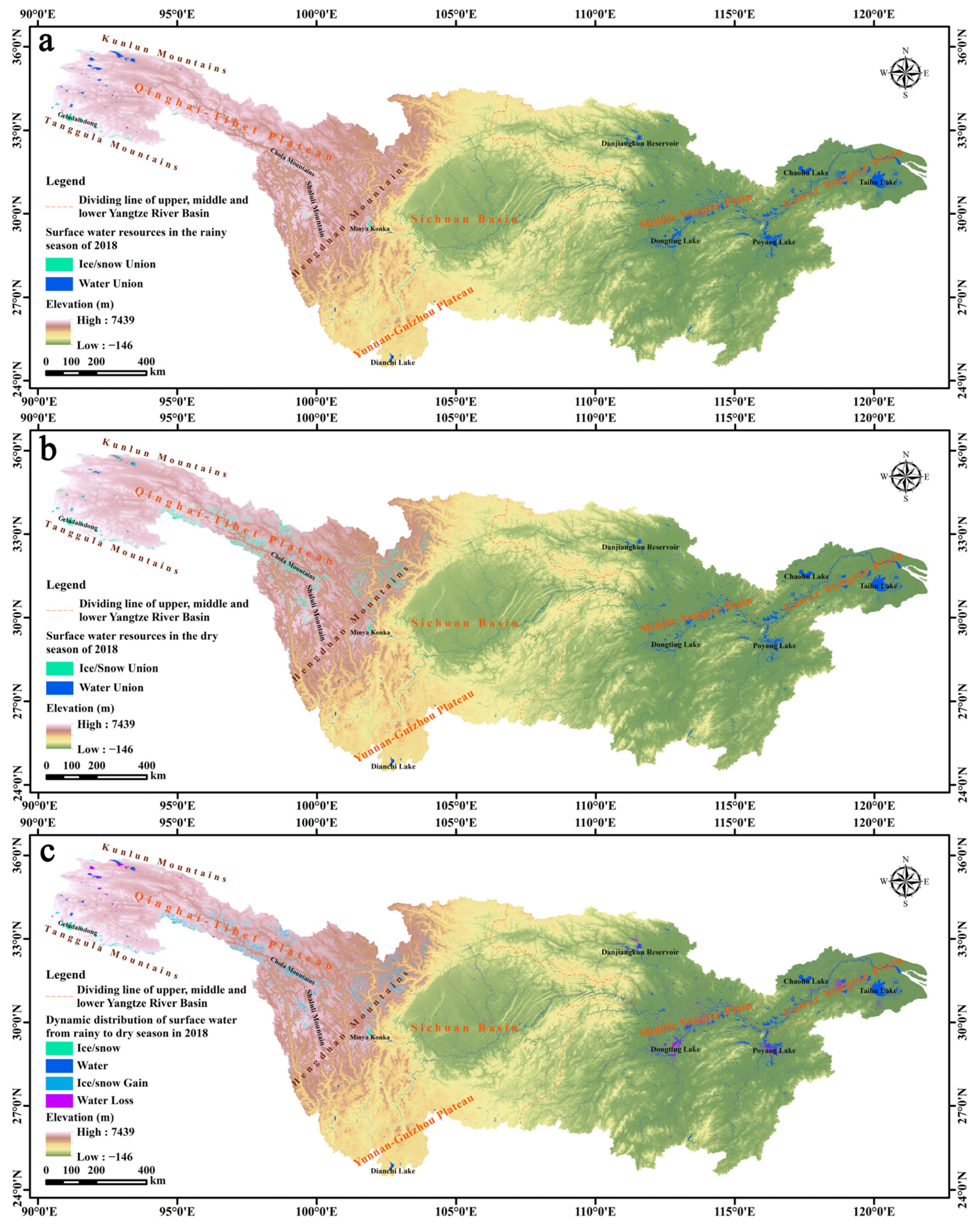
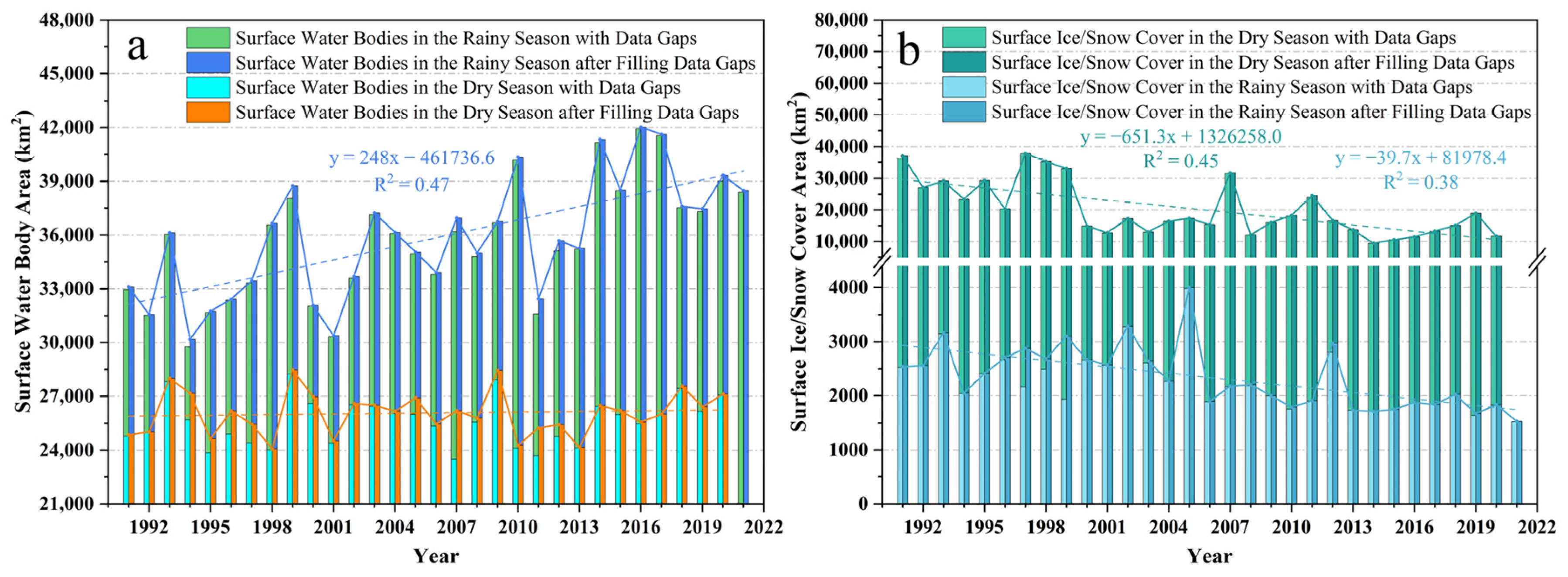
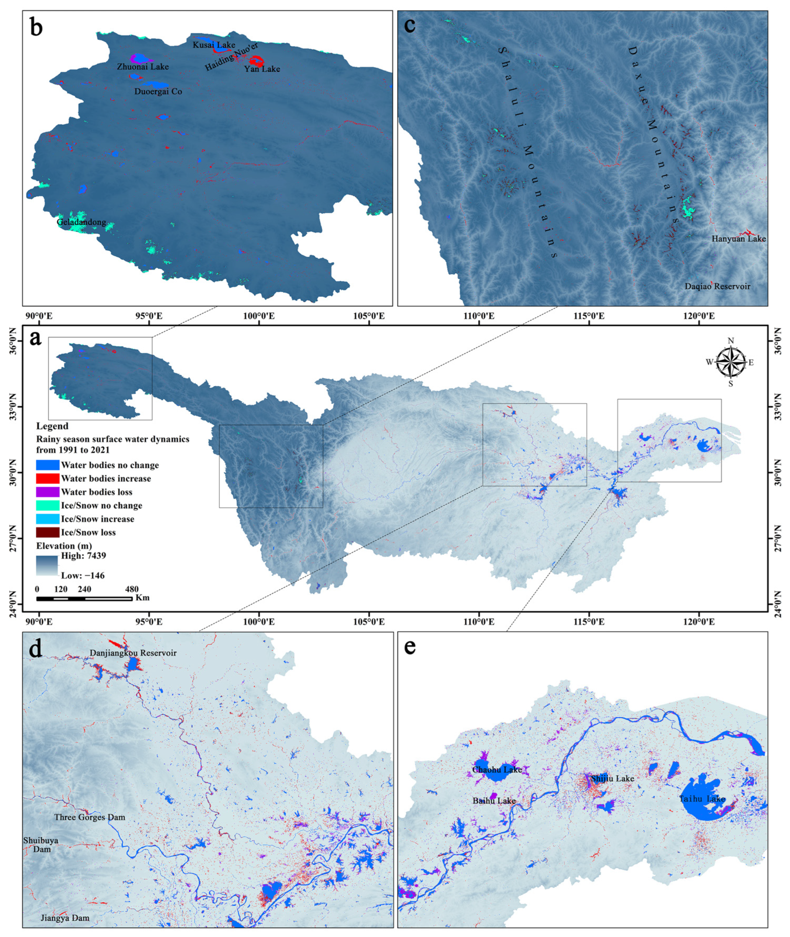
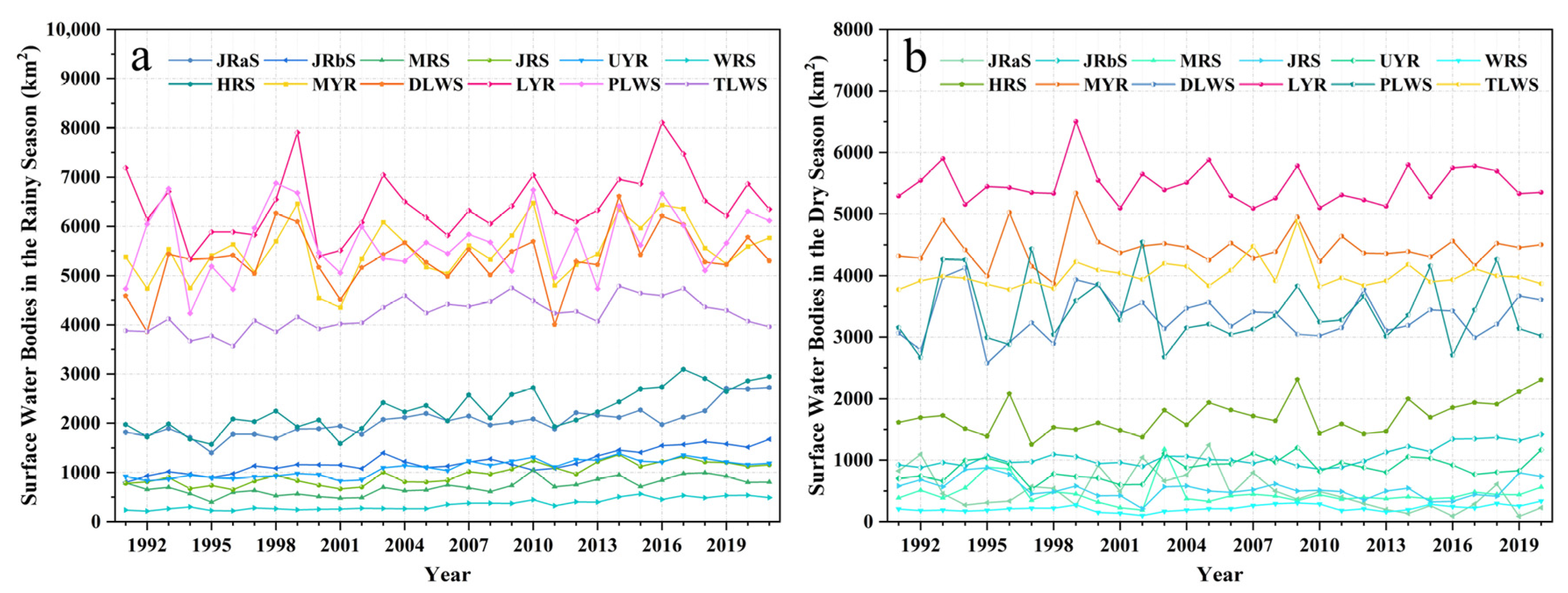
3.2. Spatial Distribution and Dynamic Changes of Surface Water Resources

The distribution of surface water bodies and surface ice/snow cover in the rainy and dry seasons in 2018 are shown in Figure 6a and Figure 6b, respectively. Surface water bodies were mainly distributed in the plains of the middle and lower reaches of the Yangtze River, where the Middle–Lower Yangtze Plain was crisscrossed by river branches and dotted with lakes. This is the most densely distributed area of lakes in China, containing four of China’s five major freshwater lakes, namely Poyang Lake, Dongting Lake, Taihu Lake and Chaohu Lake. The surface water bodies in the upper Yangtze River region mainly cover the main stream and its tributaries, some large reservoirs and lakes (e.g., Dianchi Lake in Yunnan–Guizhou Plateau) and lake groups in the source area of the Yangtze River. Surface ice/snow cover was mainly distributed in the Qinghai–Tibet Plateau and Hengduan Mountains. Ice/snow cover in the rainy season could be regarded as permanent ice/snow, which was concentrated in the high-altitude (average altitude > 5000 m) mountainous areas of the Qinghai–Tibet Plateau and Hengduan Mountains (Figure 6a). Specifically, the Geladandong Snow Mountain Group in the Tanggula Mountains of the Qinghai–Tibet Plateau, the Chola Mountains in the northern section of the Shaluli Mountains, the snow-capped mountains of the Shaluli Mountains on the southeastern edge of the Tibetan Plateau, and the Gongga Mountain in west-central Sichuan Province.

From the perspective of dynamic distribution, the changes in surface water bodies from the rainy to the dry season during the year were manifested as a decrease in river flow, with some rivers experiencing flow interruption and a reduction in the area of lakes, wetlands and reservoirs (Figure 6c). The shrinking area of lakes was relatively concentrated in the lakes at the source of the Yangtze River, Danjiangkou Reservoir, coastal lakes in the middle and lower reaches of the Yangtze River, Dongting Lake, Poyang Lake and the Shuiyang River Basin. In addition to the sharp reduction in surface water sources, the freezing and snow-covered rivers and lakes in the Qinghai–Tibet Plateau also led to the reduction in surface water bodies. In contrast, the increase in surface ice/snow cover mainly came from seasonal snowfall and was mainly distributed in plateau lakes and mountainous areas of the Qinghai–Tibet Plateau and Hengduan Mountains.

Surface water bodies and ice/snow cover in the YRB during the rainy and dry seasons from 1991 to 2021 were obtained before and after the implementation of the data gap-filling procedure outlined in Section 2.3.3, as shown in Figure 7a,b. The subsequent data analysis was based on the dataset with gaps filled. In the process of data gap filling, we found that the areas with data gaps were mainly located in the middle and upper reaches of the YRB, and mainly concentrated in the junction areas of the first and second terraces; namely, the areas between Sichuan Basin and Western Sichuan Plateau, and between Yunnan–Guizhou Plateau and Hengduan Mountains. The amount of data filling reflected the degree of missing data to some extent. From the perspective of inter-annual variation, surface water resources were in great dynamic changes. During the period 1991–2021, the minimum and maximum areal extents of the rainy season surface water bodies in the YRB were 30,176.1 km² in 1994 and 42,013.9 km² in 2016, respectively. The maximum and minimum values of the dry season surface ice/snow coverage were 37,804.3 km² in 1997 and 9405.6 km² in 2014, respectively. The peak years (e.g., 1993, 1999, 2003, 2007, 2010, 2014, 2016, and 2020) and valley years (e.g., 1994, 2001 and 2011) of surface water body area (SWBA) for the YRB in the rainy season were consistent with the flood and drought years in the Yangtze River Yearbook. The dry season peak years (e.g., 1993, 1999, 2009, and 2018) and valley years (e.g., 1995, 1998, 2001, 2010, and 2013) for SWBA in the YRB could also be traced in the Yangtze River Yearbook. In addition, the YRB also experienced severe pluvial floods in 1998 and 2017. Previous studies and statistical data showed that snow cover in winter and spring on the Qinghai–Tibet Plateau was positively correlated with the subsequent summer rainfall in the middle and lower reaches of the Yangtze River [57,58]. Comparing Figure 7a with Figure 7b, in addition to climate anomalies (e.g., the western pacific subtropical high, and the 1997 El Nino event), the unusually large areal extent of the dry season surface ice/snow cover in 1997 was also considered to have contributed to the subsequent rainy season flood in 1998. The surface water bodies generally displayed an increasing trend in the rainy season (+248.0 km²·yr⁻¹), and the surface water body changes in the dry season were relatively stable (+11.6 km²·yr⁻¹). The surface ice/snow cover showed a decreasing trend in both rainy and dry seasons, with decreasing rates of 39.7 km²·yr⁻¹ and 651.3 km²·yr⁻¹, respectively.

Figure 8a shows the spatial changes of surface water in the entire YRB during the rainy season from 1991 to 2021. As shown in Figure 8b, in addition to the shrinkage of Zhuonai Lake (it expanded rapidly in the early stage and caused a large-scale retreat of the lake shoreline after its collapse in September 2011), the overall SWBA in the source region of the Yangtze River (SRYR) increased significantly, manifested by an increase in river width and expansion of lake area. Among them, the areas of Kusai Lake, Haiding Nuo’er and Yan Lake have expanded significantly, especially Yan Lake. The overall surface ice/snow coverage area has decreased, with significant glacier retreat in the Daxue Mountains and Shaluli Mountains, as shown in Figure 8c. In the upper and middle reaches of the Yangtze River, due to the construction and operation of a series of water conservancy projects in the main stream and tributaries of the Yangtze River, the controlled storage of reservoirs and dams has increased the surface water area to a certain extent, such as the Hanyuan Lake (an artificial lake formed by the construction of Pubugou Hydropower Station on the Dadu River in 2009) and Daqiao Reservoir (first impounded in 1999) in Figure 8c, and the Three Gorges Dam (first impounded in 2003), Shuibuya Dam (first impounded in 2006) and Jiangya Reservoir (first impounded in 1998) in Figure 8d. In addition, the Danjiangkou Reservoir area in 2021 has increased significantly compared with that in 1991 (mainly due to the increase in dam height of Danjiangkou Reservoir in 2013). It can be seen from Figure 8d,e that the lakes along the middle and lower reaches of the Yangtze River have experienced varying degrees of SWBA reduction, among which the waters near Chaohu Lake (the former Baihu Lake has now been completely reclaimed), the western waters of Shijiu Lake, and the southeast waters of Taihu Lake are more obvious, and most of the surface water bodies in these areas have disappeared due to the reclamation of lakes for farmland. The increase in construction land and the development of riverbanks have also led to the reduction in SWBA in the middle and lower reaches of the Yangtze River.

Due to the comprehensive influence of climate, water vapor source, terrain and other factors, hydrological elements are unevenly distributed in the YRB, which has caused frequent floods and droughts in the basin over a long period. To explore the specific dynamic changes of surface water bodies in the YRB, the 12 water systems defined by the CWRC shown in Figure 2 were taken as the research objects and the dynamic changes of surface water bodies in the rainy and dry seasons in their respective basins from 1991 to 2021 were shown in Figure 9a and Figure 9b, respectively. The rainy season average SWBA of TLWS (11.7%), LYR (18.0%), MYR (15.3%), DLWS (14.9%), PLWS (15.9%), and HRS (6.3%) in the middle and lower Yangtze River region accounted for 82.2% of the total SWBA in the entire YRB. Inter-annual changes in SWBA in the DLWS, PLWS, MYR and LYR fluctuated greatly, indicating their vulnerability to floods and droughts. Rainy season fluctuation in surface water bodies was also marked in the TLWS, HRS, JRaS, MRS and JRS. In comparison, the variations in SWBA for the UYR, JRbS and WRS were relatively stable. The SWBA in the JRaS, JRbS, MRS, JRS, and HRS showed an increasing trend, which might be due to the melting of glaciers on the Qinghai–Tibet Plateau and Hengduan Mountains, as well as the construction of water storage projects in the middle and upper Yangtze River region. The peak and valley values for SWBA in each sub-basin also reflected regional historical hydrological events. The average SWBA for the TLWS (15.4%), LYR (21.0%), MYR (17.1%), DLWS (12.8%), PLWS (13.1%) and HRS (6.6%) in the dry season accounted for 86% of the total SWBA of the YRB. The maximum value years of dry season SWBA for LYR, MYR, TLWS and HRS were relatively concentrated in 1999 and 2009. Although the source of surface water bodies in the dry season was greatly reduced, the dynamics of surface water bodies still reflected water abundance and scarcity to a certain extent.

In addition to obtaining information on the spatial location, areal extent, lake shape, and river width of surface water, elevation data of surface water and ice/snow coverage could also be obtained. Figure 10 shows the spatial distribution of seasonal and permanent surface water bodies and ice/snow cover in the YRB in 2020. From the statistical distribution of longitude and latitude in Figure 10b,c, as well as the statistics of elevation data in Figure 10h, surface water bodies are mainly distributed in low-altitude areas below 100 m, with longitudes ranging from 111° E to 121° E and latitudes ranging from 25.7° N to 33.4° N. Four peaks in longitude corresponded to Dongting Lake, Poyang Lake, Chaohu Lake and Taihu Lake, among which surface water bodies in the Dongting Lake and Poyang Lake basins change dramatically during the year and change little in the Taihu Lake basin (Figure 10d–g). Surface ice/snow cover is mainly distributed in high-altitude areas above 3000 m, with longitudes ranging from 90.6° E to 104.6° E and latitudes ranging from 28.6° N to 35.7° N. The variation in surface ice/snow cover mainly occurs at an altitude of 4000–5000 m, accounting for 85% of the total seasonal surface ice/snow cover. Permanent surface ice/snow cover is distributed at an altitude of over 5000 m, and the two peaks in longitude correspond to the Geladandong Snow Mountain and Gongga Snow Mountain, respectively (Figure 6c).

The temporal changes in seasonal and permanent surface water in the sub-basins of the YRB from 1991 to 2020 are presented in Figure S3. Inter-annual changes in seasonal SWBA in the PLWS, DLWS, MYR and LYR fluctuated greatly (Figure S3a). The maximum values for seasonal SWBA in the PLWS, DLWS, LYR, MYR and HRS were mainly observed in 1998, 2010 and 2016, with the maximal areas of surface water bodies occurring in the rainy season and the minimal areas of surface water bodies occurring in the dry season. In Figure S3b, the variation in permanent surface water bodies in the PLWS, DLWS and MYR fluctuated significantly before 2003, and became less severe after 2003, which might be related to the regulation of surface water by the Three Gorges Dam [59]. Except for extreme values in 1996 and 2009, the permanent surface water bodies in the HRS changed gently and exhibited a steady upward trend after 2012. Permanent surface water bodies in the JRaS fluctuated greatly, while those in the JRbS changed gradually and generally presented an increasing trend. Among all the water systems in the YRB, the smallest difference between the average rainy season surface water bodies (4216.1 km²) and average permanent surface water bodies (3774.8 km²) was for the TLWS. Both seasonal and permanent surface water bodies in the YRB showed an increasing trend, with growth rates of 179.5 km²·yr⁻¹ and 80.8 km²·yr⁻¹, respectively (Figure 11a). The surface ice/snow cover was distributed in the JRaS, JRbS, MRS and JRS, and was mainly concentrated in the JRaS, JRbS, and MRS, as shown in Figure 11b,c. Both seasonal and permanent ice/snow cover showed a decreasing trend, with change rates of −603.5 km²·yr⁻¹ and −35.2 km²·yr⁻¹, respectively.

3.3. Mechanisms of Surface Water Resource Change

According to the dynamic changes of surface water extracted in the past 30 years, surface water bodies generally present an upward trend, with frequent alternation of “abundant and dry” years and extreme situations of continuous drought and flood, which has extremely adverse effects on the development of the Yangtze River Economic Belt and people’s lives. To understand the mechanism of surface water change, multiple linear stepwise regression analysis was applied to analyze the impact of climate change on surface water. Meteorological and hydrological factors used as independent variables were total precipitation in the rainy/dry season (X1), average air temperature in the rainy/dry season (X2), average surface skin temperature in the rainy/dry season (X3), total evaporation in the rainy/dry season (X4) and total surface storm runoff in the rainy/dry season (X5). The spatial distribution of meteorological data and the statistics of the 12 water systems in the YRB during the rainy season are presented in Figures S4–S7 and Tables S3–S6, respectively. The areal extents of surface water were used as the dependent variables, namely SWBA in the rainy/dry season (Y1) and surface ice/snow cover area in the rainy/dry season (Y2). Among them, surface water bodies in the rainy season and surface ice/snow cover in the dry season were the main research objects. In this paper, multiple linear stepwise regression analysis was carried out separately for each of the 12 river systems in the YRB. The statistical models describing the relationship between the surface water area and hydro-meteorological elements, together with the associated significance level and R² are presented in

Table 2. Relationships between surface water and hydro-meteorological elements.

Water System	Surface Water Bodies in the Rainy Season	Surface Ice/Snow in the Dry Season
YR	Y1YR = 7061.97 + 34.28 × X1YR (R2 = 0.58, p < 0.05)	—
JRaS	(1) Y1JRaS = −568.44 + 8.2 × X4JRaS (R2 = 0.45, p < 0.001) (2) Y1JRaS = −942.08 + 7.33 × X4JRaS + 139.55 × X3JRaS (R2 = 0.51, p < 0.05)	Y2JRaS = −7885.14 − 1267.77 × X3JRaS (R2 = 0.42, p < 0.05)
JRbS	Y1JRbS = −2825.53 + 307.27 × X3JRbS (R2 = 0.33, p < 0.05)	Y2JRbS = 6458.02 − 1565.74 × X3JRbS (R2 = 0.19, p < 0.05)
MRS	Y1MRS = 338.03 + 2.51 × X5MRS (R2 = 0.32, p < 0.001)	Y2MRS = 3918.48 − 1155.34 × X3MRS (R2 = 0.26, p < 0.05)
JRS	Y1JRS = −2724.16 + 1.09 × X1JRS + 153.68 × X2JRS (R2 = 0.44, p < 0.05)	—
UYR	(1) Y1UYR = 675.79 + 2.86 × X5UYR (R2 = 0.43, p < 0.001) (2) Y1UYR = −1993.45 + 125.6 × X2UYR + 2.73 × X5UYR (R2 = 0.55, p < 0.05)	—
WRS	(1) Y1WRS = 126.52 + 1.56 × X5WRS (R2 = 0.31, p < 0.05) (2) Y1WRS = −2218.12 + 119.53 × X2WRS + 1.52 × X5WRS (R2 = 0.51, p < 0.05)	—
HRS	Y1HRS = 1646.38 + 8.5 × X5HRS (R2 = 0.28, p < 0.05)	—
MYR	Y1MYR = 4644.16 + 5.05 × X5MYR (R2 = 0.28, p < 0.001)	—
DLWS	Y1DLWS = 2867.73 + 2.51 × X1DLWS (R2 = 0.32, p < 0.001)	—
LYR	Y1LYR = 4124.35 + 2.42 × X1LYR (R2 = 0.46, p < 0.001)	—
PLWS	Y1PLWS = 2888.83 + 2.52 × X1PLWS (R2 = 0.49, p < 0.001)	Y1PLWS = 2787.17 + 3.59 × X5PLWS (R2 = 0.33, p < 0.001)
TLWS	—	—

. It should be noted that due to the potential multicollinearity, average air temperature and average surface skin temperature cannot be used as variables simultaneously to construct regression models.

Overall, the changes in surface water bodies in the YRB during the rainy season were mainly related to precipitation, and the driving factors of surface water body change varied among different water systems. Two regression models were used to describe the relationship between SWBA and meteorological elements during the rainy season in the JRaS. Comparing model 1 with model 2, the areal extent of rainy season surface water bodies in the JRaS was positively correlated with the total evaporation in the rainy season. In fact, the total evaporation in the JRaS was the result of a combination of meteorological factors (e.g., light, air temperature, wind speed and humidity), and ultimately showed a significant positive correlation with the rainy season SWBA in that water system. In addition, the SWBA in the JRaS during the rainy season was positively correlated with the average surface skin temperature in the rainy season, while the dry season surface ice/snow cover in the JRaS was negatively correlated with the dry season average surface skin temperature. Surface skin temperature had more influence on variation in the surface water bodies in the JRbS than that in the JRaS. Surface water bodies in the JRS showed a positive relationship with both total precipitation and average air temperature during the rainy season, indicating that in addition to precipitation, temperature also contributed to changes in surface water bodies in the JRS. A possible explanation for this is that the increase in average air temperature in the rainy season accelerated the melting of ice/snow in the upper reaches of the Jialing River, resulting in an increase in the SWBA of the JRS.

Two regression models were used to describe the relationship between SWBA in the UYR during the rainy season and meteorological elements. Comparing model 1 and model 2, when storm surface runoff was used as the only independent variable in the regression analysis, the R² value was 0.43; this increased to 0.55 after average air temperature was added to model 1. These results indicated that storm surface runoff could explain 43% of the change in SWBA in the UYR and average air temperature could explain 12% of this change. Similarly, regression models for the variation in SWBA in the WRS during the rainy season indicated that 51% of this variation could be explained by storm surface runoff (31%) and average air temperature (20%). The rainy season SWBAs for the MRS, UYR, HRS and MYR were positively correlated with total surface storm runoff; the upper reaches of MRS and HRS were extremely vulnerable to geological hazards caused by storm-water runoff such as mountain torrents and debris flows [60,61]. The regression model for the change in surface water bodies in the HRS in the rainy season had a relatively low R² value, which might be due to the fact that the middle route of the South-to-North Water Diversion Project transferred water from Danjiangkou Reservoir in the middle and upper reaches of the Han River. The low R² value of the regression model for the surface water bodies in the MYR during the rainy season might be due to its complex water regime. For example, the main stream of the Yangtze River is naturally connected to Dongting Lake, which plays a role in conserving water sources and regulating the water level of the Yangtze River. When the water level in the main stream was lower than that in Dongting Lake, the lake water flowed into the Yangtze River, which increased the water volume. When flooding occurred in the main stream of the middle reaches of the Yangtze River, water poured back into Dongting Lake to reduce the flood peak.

The rainy season SWBAs in the DLWS, LYR and PLWS were positively correlated with total rainy season precipitation in their respective drainage basins. The regression model describing the relationship between the rainy season SWBA and its corresponding climate factors in the TLWS failed to pass the significance test. This is closely related to the government regulation of surface water bodies in the TLWS, which is the key area to implement the national strategy for the integrated development of the Yangtze River Delta. Specifically, floods caused by continuous rainfall in the rainy season were discharged into the Yangtze River in the north, Huangpu River in the east and Hangzhou Bay in the south. In case of drought in the rainy season, the surface water from the Yangtze River could be introduced into the TLWS to meet the water demand for living, production and ecology.

The change in surface ice/snow cover in the JRaS, JRbS and MRS during the dry season was negatively correlated with the average surface skin temperature, especially in the JRaS. In addition, factors driving the changes in surface water bodies might differ between seasons; for example, these factors differ between the rainy and dry seasons in the PLWS.

In general, the regression analysis results indicated that the changes in surface water in the YRB and its 12 water systems were not only affected by meteorological and hydrological factors but also by human activities that influenced the distribution of water resources.

4. Discussion

4.1. Extraction of Surface Water Resources throughout the Yangtze River Basin

Based on the GEE platform, multi-date composite change detection was performed by utilizing dense time stacks of Landsat imagery. Unlike previous studies of annual surface water changes [54], here we extracted surface water (i.e., surface water and ice/snow cover) in the rainy and dry seasons of the entire YRB separately to obtain accurate surface water information. Cloud masking was applied to each individual image in the selected image collections. However, while this procedure could mask out pixels with high cloud scores (i.e., thick clouds), thin clouds and haze [62] as well as shadow areas formed by thick cloud cover were not removed, which might affect the subsequent quality of composite images. Therefore, high-precision detection algorithms for thin clouds and cloud shadows are needed. Spectral indices and DEM data were added as bands to the selected image collections, which not only expanded the extracted surface water information but also improved the accuracy of surface water extraction by introducing multi-dimensional features. For the national-scale study area, more than 55,000 Landsat scenes were included in the image composites in the rainy and dry seasons during the period 1991–2021. With the support of the GEE, the time cost required for the data pre-processing was greatly reduced. Cloud cover mainly caused by weather conditions might have led to data gaps in the composite images. In order to minimize the deviation from the actual truth value of the missing area, an approach of filling the missing parts of the single-year composite image was proposed by constructing three-year image mean data (the single year was included in the three-year). Fortunately, among all the rainy season and dry season composite images during the period 1991–2021, the proportion of missing data was relatively low and the proportion of surface water resources included in the missing part was even lower (less than 5%), thus having little impact on the overall study. Similarly, the available pixels of Landsat series image data involved in image composites might show uncertainty because of cloud cover, resulting in a deviation from the real value to the actual situation, as explained in Section 2.3.3. This was mainly why, to minimize uncertainty, we applied the mean reducer to the integrated image collections. Problems with the sensor itself also affected the image synthesis quality and the extraction of surface water information. The Landsat-7 Enhanced Thematic Mapper Plus (ETM+) airborne SLC malfunctioned on 31 May 2003, resulting in data gaps in the images acquired thereafter (i.e., Landsat 7 ETM+ SLC-off data). Besides, there are differences in spectral response between different remote sensors, even different sensors of the same satellite series have differences in radiation, which might affect the surface water extraction. Thus, the Landsat series imagery selected for our study was Landsat 5 TM (1991–2011) and Landsat 8 OLI (2013–2021) image data, as well as the only available Landsat 7 ETM+ image data in 2012. There were obvious spectral disturbances in Landsat 5 TM image data from May 2001 to March 2002 in the study area, and the approach here was to combine Landsat 5 TM data with Landsat 7 ETM+ data to extract the rainy and dry season surface water information in 2001. The results showed that the influence of data gaps in the Landsat 7 image data in 2012 was greater than that of the spectral perturbation in 2001, although a gap-filling algorithm was applied to fill the scan gaps in the SLC-off data. Further study might be required that combines other available image data to obtain accurate surface water information in 2012.

For the construction of sample datasets, some previous studies directly selected samples from the existing land use/land cover (LULC) products to monitor LULC changes and applied the same sample dataset for each year to reduce the costs in labor and time. However, samples in this way are most likely pixels with no change in land use type and ignore the pixel features in the area where land use transition might occur, which will result in an imbalanced classification dataset. Here, based on manual visual interpretation, we deployed sample datasets using MNDWI single-band grayscale images as references. To extract rainy and dry season surface water resources in the YRB from 1991 to 2021, a total of 22 sample datasets for the rainy and dry seasons were deployed in every three-year period from 1991 to 2021. In terms of the GEE, due to the large number of pixels in our computation, a “computation time out” error might arise. The way to allow the computation to succeed was to increase the scale parameter. However, this may have resulted in a large deviation from the calculation results at the original resolution of the image data source (30 m). To address this issue, the classification results for surface water were exported to the local ENVI 5.3 software for raster-to-vector conversion, and then transferred to ArcGIS 10.6 software for area calculation, mapping and the extraction of the derived data (such as seasonal surface water bodies, and permanent surface ice/snow).

4.2. Comparative Analysis with Existing Surface Water Datasets

In this section, we compare the surface water extraction results obtained using our method with the JRC Yearly Water Classification History (Version 1.4) and GLIMS Current datasets. The JRC Yearly Water Classification History dataset contains a year-by-year classification of the seasonality of surface water, divided into seasonal and permanent surface water bodies based on the occurrence values detected throughout the year. The GLIMS Current dataset was created by repeatedly surveying the world’s estimated glaciers, which were regarded as permanent ice/snow. The permanent water and seasonal water derived in this study were compared with the JRC Yearly Water Classification History and GLIMS Current datasets, as shown in Figure 12. Comparison analysis for surface water in the SRYR, the typical area of DLWS and PLWS, and the Qingyi–Shuiyang River System (QSRS) were conducted in 1996, 2006 and 2016 respectively. Although there were differences in the definition of seasonal and permanent surface water, the contours and shapes of the surface water obtained by the two methods were comparable. For the surface water in the SRYR, the difference was mainly reflected in the lake water state. Because the expert system treated ice as an invalid observation, the observation period for JRC surface water corresponded to the unfrozen months only. Therefore, the lakes in the SRYR were considered to be permanent surface water, while our results showed the actual situation of lake water being frozen and snowbound as the season changed from the rainy season to the dry season.

Overall, the permanent ice/snow cover area derived using our method was similar to that from the GLIMS data, and the difference was mainly in seasonal surface water. The areal extent of seasonal surface water we derived was smaller than that of JRC seasonal surface water. The main reason for this was probably the differences in the time phase of surface water extraction and the definition of seasonal surface water. The rainy season (May–October) and dry season (November to April of the next year) were not divided by calendar year. Seasonal surface water here was derived by calculating the symmetrical difference between the rainy and dry season surface water, and our surface water data set was extracted from the image composites aggregated by reducing the image collections with a mean reducer. Thus, some of the water pixels were weakened. The seasonal surface water of the JRC surface water dataset appeared more like the maximum pixel value of water bodies throughout the year after removing permanent surface water. That is to say, surface water detected in fewer than 12 months of the year was seasonal surface water. The JRC surface water was affected by data gaps caused by the SLC failure in 2003, resulting in an error in the distinction between permanent and seasonal surface water, as shown in the typical area of DLWS and the lake area of QSRS in Figure 12b, even for the typical area of the PLWS in 2016 (Figure 12c), there were still traces of striping. In addition, there were obvious missing data in the JRC yearly surface water in the YRB in 1996, which were not shown in Figure 12. In view of these two issues, we proposed reasonable and feasible solutions to assist in the extraction of surface water. Further study is required to extract extreme values of water pixels during the rainy and dry seasons and explore the possible impacts of floods and droughts on the areal extent of surface water.

4.3. Limitatios of Analyzing the Driving Fators of Dynamic Changes in Surface Water

The relationships between surface water area and hydro-meteorological elements in 12 water systems in the YRB were estimated by utilizing multiple linear stepwise regression analyses. Unfortunately, quantitative indicators of human activities (e.g., water consumption, water supply for agriculture, industry, domestic and ecological environments) were not included in the regression analysis. There are several reasons for this: the lack of statistical data for some years, especially before 1997; some statistical indicators in the statistical system have changed; the statistics are compiled on an annual basis, which differs from the time phase of our study. In addition, there has been a lack of research on the response mechanism and quantitative identification of surface water under the influence of human activities, such as the operation of water conservancy projects and government regulation of surface water. In particular, the Three Gorges Dam has played a positive role in reducing the flood control pressure in the middle and lower reaches by blocking flood flows and reducing the flood peak during the rainy season, and alleviating drought effects by increasing water release and water supplementation during the dry season. Although the results of regression analysis revealed that changes in surface water were affected by both climatic factors and human activities, the response mechanism and quantitative identification of surface water under the influence of human activities should be further studied.

Multiple linear regression attempts to estimate the relationship between a response variable and two or more predictor variables by fitting a linear equation, which does not mean that there is a strict causal relationship between the dependent variable and independent variables [63]. As discussed previously, the rainy season SWBA in the UYR and WRS was positively correlated with the rainy season average air temperature. The possible explanation might be that the rainy season average air temperature in the UYR and WRS were highly consistent with the average temperature in the rainy season for the entire YRB (R² = 0.72 and 0.84, respectively). As the temperature rises, the amount of ice/snow melting water increases, and then feeds back to the UYR, resulting in an increase in SWBA. For the WRS, the saturated vapor pressure increases significantly with the rise in average air temperature, making the air more capable of holding water vapor and greatly increasing the possibility of heavy precipitation, showing a positive correlation with the SWBA in the WRS. Thus, the change in the rainy season average air temperature in the UYR and WRS was largely affected by the warming background of the entire YRB, and the total surface storm runoff was considered to be the main driving factor for the dynamic change in SWBA in the UYR and WRS. In relation to surface water bodies in the WRS, Zhu et al. [64] conducted a study on water area changes and climate effects in the WRS during the period 1983–2015. Although there were differences in the time phase of the data, the correlation between surface water area and average temperature was echoed by the results of our regression analysis for the WRS. Therefore, in the multivariate regression analysis, in addition to testing the significance of the regression equation, it is necessary to combine specific environment in which the variables are located to further determine the driving factors.

5. Conclusions

To better understand the dynamics of surface water, this paper analyzed surface water bodies and ice/snow cover in the rainy and dry seasons separately, rather than just exploring annual surface water bodies. Supported by the GEE, we developed a multi-date composite image change detection technique utilizing dense time stacks of Landsat satellite imagery and applied the RF algorithm to extract rainy and dry season surface water in the YRB during the period 1991–2021. The spatial distribution, temporal changes in surface water bodies and ice/snow cover, and their relationships to climatic and anthropogenic drivers were analyzed. The proposed method for monitoring the dynamics of surface water in this study can provide a reference for similar studies at large regional or national levels.

Our results suggested that the inter-annual variation in surface water in the YRB was in great dynamics and the spatiotemporal distribution of surface water was very uneven. Rainy season surface water bodies generally showed an increasing trend (+248.0 km²·yr⁻¹), while surface ice/snow cover in both rainy and dry seasons displayed a decreasing trend, with decreasing rates of 39.7 km²·yr⁻¹ and 651.3 km²·yr⁻¹, respectively. The inter-annual and intra-annual variations in SWBA in the DLWS, PLWS, MYR and LYR fluctuate greatly, reflecting their vulnerability to flood and drought disasters. In addition, the correlation analysis between areal extents of surface water and hydro-meteorological elements indicates that precipitation is the main cause of the changes in the surface water bodies, and surface ice/snow cover is negatively correlated with the average surface skin temperature. The climate-related factors driving surface water changes present spatial differences between secondary river systems, highlighting the complexity of surface water dynamics. This research helps not only to systematically explore the spatiotemporal distribution and variation characteristics of surface water in the YRB in the last three decades but also to better understand mechanisms driving the impacts of climate change and human activities on the dynamics of surface water.

References

1. Salman, M.A. United Nations General Assembly Resolution: International Decade for Action, Water for Life, 2005–2015. Water Int. 2005, 30, 415–418. [Google Scholar] [CrossRef]
2. Goldblatt, R.; You, W.; Hanson, G.; Khandelwal, A. Detecting the Boundaries of Urban Areas in India: A Dataset for Pixel-Based Image Classification in Google Earth Engine. Remote Sens. 2016, 8, 634. [Google Scholar] [CrossRef]
3. Mekonnen, M.M.; Hoekstra, A.Y. Four billion people facing severe water scarcity. Sci. Adv. 2016, 2, e1500323. [Google Scholar] [CrossRef] [PubMed]
4. WWAP (UNESCO World Water Assessment Programme). The United Nations World Water Development Report 2019: Leaving No One Behind; UNESCO: Paris, France, 2019. [Google Scholar]
5. UNESCO. The United Nations World Water Development Report 2020: Water and Climate Change; UNESCO: Paris, France, 2020. [Google Scholar]
6. Vörösmarty, C.J.; Green, P.; Salisbury, J.; Lammers, R.B. Global water resources: Vulnerability from climate change and population growth. Science 2000, 289, 284–288. [Google Scholar] [CrossRef] [PubMed]
7. Huang, C.; Chen, Y.; Zhang, S.; Wu, J. Detecting, Extracting, and Monitoring Surface Water From Space Using Optical Sensors: A Review. Rev. Geophys. 2018, 56, 333–360. [Google Scholar] [CrossRef]
8. Woodcock, C.E.; Macomber, S.A.; Pax-Lenney, M.; Cohen, W.B. Monitoring large areas for forest change using Landsat: Generalization across space, time and Landsat sensors. Remote Sens. Environ. 2001, 78, 194–203. [Google Scholar] [CrossRef]
9. Sawaya, K.; Olmanson, L.G.; Heinert, N.J.; Brezonik, P.L.; Bauer, M.E. Extending satellite remote sensing to local scales: Land and water resource monitoring using high-resolution imagery. Remote Sens. Environ. 2003, 88, 144–156. [Google Scholar] [CrossRef]
10. Pittman, K.; Hansen, M.C.; Becker-Reshef, I.; Potapov, P.V.; Justice, C.O. Estimating Global Cropland Extent with Multi-year MODIS Data. Remote Sens. 2010, 2, 1844–1863. [Google Scholar] [CrossRef]
11. Davranche, A.; Lefebvre, G.; Poulin, B. Wetland monitoring using classification trees and SPOT-5 seasonal time series. Remote Sens. Environ. 2010, 114, 552–562. [Google Scholar] [CrossRef]
12. Pu, R.; Bell, S. Mapping seagrass coverage and spatial patterns with high spatial resolution IKONOS imagery. Int. J. Appl. Earth Obs. Geoinf. 2017, 54, 145–158. [Google Scholar] [CrossRef]
13. Prigent, C.; Papa, F.; Aires, F.; Jimenez, C.; Rossow, W.B.; Matthews, E. Changes in land surface water dynamics since the 1990s and relation to population pressure. Geophys. Res. Lett. 2012, 39. [Google Scholar] [CrossRef]
14. Cooley, S.; Smith, L.; Stepan, L.; Mascaro, J. Tracking Dynamic Northern Surface Water Changes with High-Frequency Planet CubeSat Imagery. Remote Sens. 2017, 9, 1306. [Google Scholar] [CrossRef]
15. Prigent, C.; Jimenez, C.; Bousquet, P. Satellite-derived global surface water extent and dynamics over the last 25 years (GIEMS-2). J. Geophys. Res. Atmos. 2020, 125, e2019JD030711. [Google Scholar] [CrossRef]
16. Zhang, D.D.; Zhang, L. Land Cover Change in the Central Region of the Lower Yangtze River Based on Landsat Imagery and the Google Earth Engine: A Case Study in Nanjing, China. Sensors 2020, 20, 2091. [Google Scholar] [CrossRef]
17. Johansen, K.; Phinn, S.; Taylor, M. Mapping woody vegetation clearing in Queensland, Australia from Landsat imagery using the Google Earth Engine. Remote Sens. Appl. Soc. Environ. 2015, 1, 36–49. [Google Scholar] [CrossRef]
18. Carroll, M.; Wooten, M.; DiMiceli, C.; Sohlberg, R.; Kelly, M. Quantifying Surface Water Dynamics at 30 Meter Spatial Resolution in the North American High Northern Latitudes 1991–2011. Remote Sens. 2016, 8, 622. [Google Scholar] [CrossRef]
19. Ying, Q.; Hansen, M.C.; Potapov, P.V.; Tyukavina, A.; Wang, L.; Stehman, S.V.; Moore, R.; Hancher, M. Global bare ground gain from 2000 to 2012 using Landsat imagery. Remote Sens. Environ. 2017, 194, 161–176. [Google Scholar] [CrossRef]
20. Pekel, J.F.; Cottam, A.; Gorelick, N.; Belward, A.S. High-resolution mapping of global surface water and its long-term changes. Nature 2016, 540, 418–422. [Google Scholar] [CrossRef]
21. McFeeters, S.K. The use of the Normalized Difference Water Index (NDWI) in the delineation of open water features. Int. J. Remote Sens. 1996, 17, 1425–1432. [Google Scholar] [CrossRef]
22. Xu, H. Modification of normalised difference water index (NDWI) to enhance open water features in remotely sensed imagery. Int. J. Remote Sens. 2007, 27, 3025–3033. [Google Scholar] [CrossRef]
23. Salomonson, V.V.; Appel, I. Estimating fractional snow cover from MODIS using the normalized difference snow index. Remote Sens. Environ. 2004, 89, 351–360. [Google Scholar] [CrossRef]
24. Choi, H.; Bindschadler, R. Cloud detection in Landsat imagery of ice sheets using shadow matching technique and automatic normalized difference snow index threshold value decision. Remote Sens. Environ. 2004, 91, 237–242. [Google Scholar] [CrossRef]
25. Tucker, C.J. Red and photographic infrared linear combinations for monitoring vegetation. Remote Sens. Environ. 1979, 8, 127–150. [Google Scholar] [CrossRef]
26. Sakamoto, T.; Van Nguyen, N.; Kotera, A.; Ohno, H.; Ishitsuka, N.; Yokozawa, M. Detecting temporal changes in the extent of annual flooding within the Cambodia and the Vietnamese Mekong Delta from MODIS time-series imagery. Remote Sens. Environ. 2007, 109, 295–313. [Google Scholar] [CrossRef]
27. Deka, P.C. Support vector machine applications in the field of hydrology: A review. Appl. Soft Comput. 2014, 19, 372–386. [Google Scholar]
28. Meng, Y.; Du, P.; Wang, X.; Bai, X.; Guo, S. Monitoring Human-induced Surface Water Disturbance around Taihu Lake since 1984 by Time Series Landsat Images. IEEE J. Sel. Top. Appl. Earth Obs. Remote Sens. 2020, 13, 3780–3789. [Google Scholar] [CrossRef]
29. Huang, X.; Xie, C.; Fang, X.; Zhang, L. Combining Pixel- and Object-Based Machine Learning for Identification of Water-Body Types from Urban High-Resolution Remote-Sensing Imagery. IEEE J. Sel. Top. Appl. Earth Obs. Remote Sens. 2015, 8, 2097–2110. [Google Scholar] [CrossRef]
30. Duan, Y.; Zhang, W.; Huang, P.; He, G.; Guo, H. A New Lightweight Convolutional Neural Network for Multi-Scale Land Surface Water Extraction from GaoFen-1D Satellite Images. Remote Sens. 2021, 13, 4576. [Google Scholar] [CrossRef]
31. Earth Engine Code Editor. Available online: http://code.earthengine.google.com (accessed on 12 July 2021).
32. Gorelick, N.; Hancher, M.; Dixon, M.; Ilyushchenko, S.; Thau, D.; Moore, R. Google Earth Engine: Planetary-scale geospatial analysis for everyone. Remote Sens. Environ. 2017, 202, 18–27. [Google Scholar] [CrossRef]
33. De Alban, J.D.T.; Connette, G.M.; Oswald, P.; Webb, E.L. Combined Landsat and L-Band SAR Data Improves Land Cover Classification and Change Detection in Dynamic Tropical Landscapes. Remote Sens. 2018, 10, 306. [Google Scholar] [CrossRef]
34. Kumar, L.; Mutanga, O. Google Earth Engine Applications Since Inception: Usage, Trends, and Potential. Remote Sens. 2018, 10, 1509. [Google Scholar] [CrossRef]
35. Breiman, L. Random Forests. Mach. Learn. 2001, 45, 5–32. [Google Scholar] [CrossRef]
36. Liu, J.; Yang, H.; Gosling, S.N.; Kummu, M.; Flörke, M.; Pfister, S.; Hanasaki, N.; Wada, Y.; Zhang, X.; Zheng, C.; et al. Water scarcity assessments in the past, present and future. Earth’s Future 2017, 5, 545–559. [Google Scholar] [CrossRef]
37. Du, Y.; Xue, H.P.; Wu, S.J.; Ling, F.; Xiao, F.; Wei, X.H. Lake area changes in the middle Yangtze region of China over the 20th century. J. Environ. Manage. 2011, 92, 1248–1255. [Google Scholar] [CrossRef]
38. Outline of the Yangtze River Delta Regional Integration Development Plan. Available online: http://www.gov.cn/zhengce/2019-12/01/content_5457442.htm (accessed on 18 August 2022).
39. Guiding Opinions of the State Council on Promoting the Development of the Yangtze River Economic Belt by Relying on the Golden Waterway. Available online: http://www.gov.cn/zhengce/content/2014-09/25/content_9092.htm (accessed on 15 August 2022).
40. Yang, J. The Historical Analysis on the Evolution of the Relationship between Economy and Ecology in the Yangtze River Economic Belt (from 1979 to 2015). Ph.D. Thesis, Zhongnan University of Economics and Law, Wuhan, China, 1 December 2018. [Google Scholar]
41. Funk, C.; Peterson, P.; Landsfeld, M.; Pedreros, D.; Verdin, J.; Shukla, S.; Husak, G.; Rowland, J.; Harrison, L.; Hoell, A.; et al. The climate hazards infrared precipitation with stations—A new environmental record for monitoring extremes. Sci. Data 2015, 2, 150066. [Google Scholar] [CrossRef]
42. Muñoz Sabater, J. ERA5-Land Monthly Averaged Data from 1981 to Present. Copernicus Climate Change Service (C3S) Climate Data Store (CDS), 2019. Available online: https://cds.climate.copernicus.eu/cdsapp#!/dataset/reanalysis-era5-land-monthly-means?tab=overview (accessed on 12 September 2022).
43. Chander, G.; Markham, B.L.; Helder, D.L. Summary of current radiometric calibration coefficients for Landsat MSS, TM, ETM+, and EO-1 ALI sensors. Remote Sens. Environ. 2009, 113, 893–903. [Google Scholar] [CrossRef]
44. Zha, Y.; Gao, J.; Ni, S. Use of normalized difference built-up index in automatically mapping urban areas from TM imagery. Int. J. Remote Sens. 2003, 24, 583–594. [Google Scholar] [CrossRef]
45. Wilson, E.H.; Sader, S.A. Detection of forest harvest type using multiple dates of Landsat TM imagery. Remote Sens. Environ. 2002, 80, 385–396. [Google Scholar] [CrossRef]
46. Skakun, R.S.; Wulder, M.A.; Franklin, S.E. Sensitivity of the thematic mapper enhanced wetness difference index to detect mountain pine beetle red-attack damage. Remote Sens. Environ. 2003, 86, 433–443. [Google Scholar] [CrossRef]
47. Jarvis, A.; Reuter, H.I.; Nelson, A.; Guevara, E. Hole-Filled SRTM for the Globe Version 4, Available from the CGIAR-CSI SRTM 90m Database. 2008. Available online: http://srtm.csi.cgiar.org (accessed on 27 May 2023).
48. Bishop, M.P.; Olsenholler, J.A.; Shroder, J.F.; Barry, R.G.; Raup, B.H.; Bush, A.B.G.; Copland, L.; Dwyer, J.L.; Fountain, A.G.; Haeberli, W.; et al. Global Land Ice Measurements from Space (GLIMS): Remote Sensing and GIS Investigations of the Earth’s Cryosphere. Geocarto Int. 2004, 19, 54–87. [Google Scholar] [CrossRef]
49. Raup, B.; Kääb, A.; Kargel, J.S.; Bishop, M.P.; Hamilton, G.; Lee, E.; Paul, F.; Rau, F.; Soltesz, D.; Khalsa, S.J.S.; et al. Remote sensing and GIS technology in the Global Land Ice Measurements from Space (GLIMS) Project. Comput. Geosci. 2007, 33, 104–125. [Google Scholar] [CrossRef]
50. Abatzoglou, J.T.; Dobrowski, S.Z.; Parks, S.A.; Hegewisch, K.C. TerraClimate, a high-resolution global dataset of monthly climate and climatic water balance from 1958–2015. Sci. Data 2018, 5, 170191. [Google Scholar] [CrossRef]
51. McNally, A.; Arsenault, K.; Kumar, S.; Shukla, S.; Peterson, P.; Wang, S.; Funk, C.; Peters-Lidard, C.D.; Verdin, J.P. A land data assimilation system for sub-Saharan Africa food and water security applications. Sci. Data 2017, 4, 170012. [Google Scholar] [CrossRef] [PubMed]
52. Hu, Y.; Hu, Y. Detecting Forest Disturbance and Recovery in Primorsky Krai, Russia, Using Annual Landsat Time Series and Multi–Source Land Cover Products. Remote Sens. 2020, 12, 129. [Google Scholar] [CrossRef]
53. Nyland, K.E.; Gunn, G.E.; Shiklomanov, N.I.; Engstrom, R.N.; Streletskiy, D.A. Land Cover Change in the Lower Yenisei River Using Dense Stacking of Landsat Imagery in Google Earth Engine. Remote Sens. 2018, 10, 1226. [Google Scholar] [CrossRef]
54. Wang, C.; Jia, M.; Chen, N.; Wang, W. Long-Term Surface Water Dynamics Analysis Based on Landsat Imagery and the Google Earth Engine Platform: A Case Study in the Middle Yangtze River Basin. Remote Sens. 2018, 10, 1635. [Google Scholar] [CrossRef]
55. Gislason, P.O.; Benediktsson, J.A.; Sveinsson, J.R. Random Forests for land cover classification. Pattern Recognit. Lett. 2006, 27, 294–300. [Google Scholar] [CrossRef]
56. Yu, X.; Hyyppä, J.; Vastaranta, M.; Holopainen, M.; Viitala, R. Predicting individual tree attributes from airborne laser point clouds based on the random forests technique. ISPRS J. Photogramm. Remote Sens. 2011, 66, 28–37. [Google Scholar] [CrossRef]
57. Wu, T.W.; Qian, Z.A. The relation between the Tibetan winter snow and the Asian summer monsoon and rainfall: An observational investigation. J. Clim. 2003, 16, 2038–2051. [Google Scholar] [CrossRef]
58. Zhang, Y.; Li, T.; Wang, B. Decadal change of the spring snow depth over the Tibetan Plateau: The associated circulation and influence on the East Asian summer monsoon. J. Clim. 2004, 17, 2780–2793. [Google Scholar] [CrossRef]
59. Peng, Y.; He, G.; Wang, G.; Cao, H. Surface Water Changes in Dongting Lake from 1975 to 2019 Based on Multisource Remote-Sensing Images. Remote Sens. 2021, 13, 1827. [Google Scholar] [CrossRef]
60. Wu, X.; Tang, S. Comprehensive evaluation of ecological vulnerability based on the AHP-CV method and SOM model: A case study of Badong County, China. Ecol. Indic. 2022, 137, 108758. [Google Scholar] [CrossRef]
61. Yang, X.; Dai, X.; Li, W.; Lu, H.; Liu, C.; Li, N.; Yang, Z.; He, Y.; Li, W.; Fu, X.; et al. Socio-Ecological Vulnerability in Aba Prefecture, Western Sichuan Plateau: Evaluation, Driving Forces and Scenario Simulation. ISPRS Int. J. Geo-Inf. 2022, 11, 524. [Google Scholar] [CrossRef]
62. Guo, Q.; Hu, H.M.; Li, B. Haze and Thin Cloud Removal Using Elliptical Boundary Prior for Remote Sensing Image. IEEE Trans. Geosci. Remote Sens. 2019, 57, 9124–9137. [Google Scholar] [CrossRef]
63. Hu, Y.; Hu, Y. Land Cover Changes and Their Driving Mechanisms in Central Asia from 2001 to 2017 Supported by Google Earth Engine. Remote Sens. 2019, 11, 554. [Google Scholar] [CrossRef]
64. Zhu, X. Preliminary Study on Water Area Changes and Climate Effects in Wujiang River Basin in Guizhou. Master’s Thesis, Guizhou Normal University, Guiyang, China, 3 June 2020. [Google Scholar]
Figure 1. An overview of the entire Yangtze River Basin (YRB): (a) the location of the YRB in China; (b) the distribution of major rivers and lakes, and topographic map of the study area. Data source: Shuttle Radar Topography Mission (http://srtm.csi.cgiar.org, accessed on 15 March 2022).
Water 16 00677 g001
Figure 2. Water system division of the YRB. From left to right: Jinsha River above Shigu (JRaS), Jinsha River below Shigu (JRbS), Minjiang River System (MRS), Upper Yangtze River (UYR), Jialing River System (JRS), Wujiang River System (WRS), Middle Yangtze River (MYR), Dongting Lake Water System (DLWS), Han River System (HRS), Lower Yangtze River (LYR), Poyang Lake Water System (PLWS), and Taihu Lake Water System (TLWS).
Water 16 00677 g002
Figure 3. Spatial distribution of total observations in the dry season for the entire YRB during the study periods: (a) Landsat 5 scenes from 1991 to 2011; (b) Landsat 8 scenes from 2013 to 2021.
Water 16 00677 g003
Figure 4. Flowchart of rainy and dry season surface water mapping and driving mechanism analysis. Surface water mapping involved data processing, deployment of sample datasets, random forest classification and data gap-filling.
Water 16 00677 g004
Figure 5. Deployment of sample points in the YRB during the rainy season from 2003 to 2005.
Water 16 00677 g005
Figure 6. Spatial distribution of surface water resources in the YRB in 2018 (a) during the rainy season and (b) during the dry season. (c) Dynamic change in surface water resources in the YRB from the rainy to the dry season in 2018.
Water 16 00677 g006
Figure 7. Surface water dynamics in the YRB during the rainy and dry seasons from 1991 to 2021. (a) Dynamics of surface water bodies. (b) Dynamics of surface ice/snow cover.
Water 16 00677 g007
Figure 8. The spatial changes of surface water in the entire YRB during the rainy season from 1991 to 2021. (a) Spatial dynamic distribution of the rainy season surface water in the YRB from 1991 to 2021. (be) Partial enlargement of the selected area in (a).
Water 16 00677 g008
Figure 9. Dynamics of surface water body in 12 water systems in the YRB during the rainy and dry seasons. (a) Dynamics of the rainy season surface water bodies from 1991 to 2021. (b) Dynamics of the dry season surface water bodies from 1991 to 2020.
Water 16 00677 g009
Figure 10. Maps of the distributions of seasonal and permanent surface water in the YRB in 2020. (a) Overall spatial distribution of seasonal and permanent surface water bodies and ice/snow cover in the YRB. Statistical distribution of surface water bodies and ice/snow cover in the YRB by (b) longitude and (c) latitude. Locally amplified spatial distribution of seasonal and permanent surface water bodies in the (d) Dongting Lake, (e) Poyang Lake, (f) Chaohu Lake and (g) Taihu Lake. (h) Statistical distribution of elevation data information on surface water bodies and ice/snow cover.
Water 16 00677 g010
Figure 11. Dynamic change trends of (a) seasonal and permanent surface water bodies, (b) seasonal and (c) permanent surface ice/snow cover in the YRB from 1991 to 2020. Notes: Permanent surface water bodies here refer to surface water that persists from May of one year to April of the next.
Water 16 00677 g011
Figure 12. Comparisons of permanent and seasonal surface water derived from our extracted rainy and dry season surface water with the JRC Yearly Water Classification History and GLIMS Current datasets. JRC PW represents permanent surface water, and JRC SW represents seasonal surface water. Comparison results in the SRYR, the typical area of DLWS and PLWS, and the QSRS in (a) 1996, (b) 2006 and (c) 2016, respectively.
Water 16 00677 g012