Characterization of Groundwater Geochemistry in an Esker Aquifer in Western Finland Based on Three Years of Monitoring Data

Abstract

This study investigated the hydrogeochemistry of a shallow Quaternary sedimentary aquifer in an esker deposition in western Finland, where distinct spatial and temporal variability in groundwater hydrogeochemistry has been observed. Field investigation and hydrogeochemical data were obtained from autumn 2010 to autumn 2013. The data were analyzed using the multivariate statistical methods principal component analysis (PCA) and hierarchical cluster analysis (HCA), in conjunction with groundwater classification based on the main ionic composition. The stable isotope ratios of δ¹⁸O and δD were used to determine the origin of the groundwater and its connection to surface water bodies. The groundwater geochemistry is characterized by distinct redox zones caused by the influence of organic matter, pyrite oxidation, and preferential flow pathways due to different hydrogeological conditions. The groundwater is of the Ca-HCO₃ type and locally of the Ca-HCO₃-SO₄ type, with low TDS, alkalinity, and pH, but elevated Fe and Mn concentrations, KMnO₄ consumption, and, occasionally, Ni concentrations. The decomposition of organic matter adds CO₂ to the groundwater, and in this study, the dissolution of CO₂ was found to increase the pH and enhance the buffering capacity of the groundwater. The mobility of redox-sensitive elements and trace metals is controlled by pH and redox conditions, which are affected by the pumping rate, precipitation, and temperature. With the expected future increases in precipitation and temperature, the buffering capacity of the aquifer system will enhance the balance between alkalinity from bioactivity and acidity from recharge and pyrite oxidation.

1. Introduction

Glaciofluvial deposits, especially eskers, are important aquifer types in the Fennoscandian Shield and in northern regions formed during the last deglaciation, e.g., in Finland, Sweden, and North America (e.g., [1,2,3,4,5]). In Finland, there are over 5000 classified groundwater areas, covering a surface area of approximately 7059 km² (Figure 1, index map), which are mainly unconfined esker aquifers. Groundwater recharge in these aquifers totals 2065 billion m³/year and the usage is 253 billion m³/year, and 65% of water consumption in Finland is supplied by groundwater [6,7,8,9,10]. Unconfined esker aquifers usually consist of well-sorted sand and gravel deposits, with the hydraulic conductivity varying between 0.001 and 0.044 m/s and the horizontal hydraulic gradient being between 0.001 and 0.006 [11]. In Finland, the groundwater table is on average between 2 and 4 m below the ground surface, but it can be as deep as 30 m below the ground surface in esker ridges. Unconfined esker aquifers are often connected to surface water bodies, i.e., lakes, rivers, ponds, wetlands [6,7,8,12], the Gulf of Bothnia [11], or the Baltic Sea [13]. Eskers can host groundwater-dependent ecosystems [14] and can be affected by human activities (e.g., [15]).

1.1. Overview of Groundwater Studies in Finland

National groundwater quality in Finland has previously been investigated, among others, by [16,17]. Lahermo et al. [17] collected over a thousand water samples across Finland in 1999 and analyzed more than 40 elements (major, minor, and trace elements, stable water isotopes δ¹⁸O and δD). They concluded that groundwater quality is controlled by geological, biological, and anthropogenic factors. Naturally occurring groundwater is characterized by high concentrations of dissolved Fe and Mn and a low pH, with 57% of wells dug into shallow Quaternary aquifers having a pH of less than 6.5. Low pH values are associated with the abundance of dissolved organic compounds or humus. Korkka-Niemi [16] examined the cumulative factors affecting water quality from regional to site-specific scales and the seasonal variation in water quality from 1421 private wells in Finland. Regional effects were caused by the natural occurrence, the aquifer characteristics, and the hydraulic conditions of the aquifer system, while site-specific effects were associated with the well conditions and anthropogenic sources of contamination. The study revealed that partly regional and partly site-specific data are affected by the redox conditions, which explain the high turbidity, color, KMnO₄ consumption, and Al, Fe, and Mn concentrations of the water.

Artimo et al. [6] characterized the hydrogeology of an esker aquifer in a 3D model to support the comprehensive understanding of the aquifer for water resources management at a managed aquifer recharge (MAR) site in southern Finland. Rossi et al. [18] investigated the connection of an esker aquifer to nearby peatland using a groundwater flow model. Ala-Aho et al. [12] and Rautio and Korkka-Niemi [7] examined groundwater and surface water interactions in esker aquifers using hydrogeochemistry, especially stable water isotopes. Okkonen and Kløve [8] assessed the temporal and spatial variations in the chemical composition of groundwater in an unconfined esker aquifer. They found that the solute concentrations decreased during and immediately after snowmelt in the spring, and a surface water connection with the aquifer was detected based on the chloride concentrations.

In coastal regions, eskers can be partly or fully covered by marine silt and clay deposits, as described in [4,11]. Overlying fine-grained layers from marine deposits often cause esker aquifers to be partly confined, preventing the free percolation of oxygen to the aquifer. Reduced conditions occur when groundwater contains less than 0.5 mg/L dissolved oxygen (DO) [19]. This can normally be found along the sides of eskers that are covered by a fine-grained layer, in stagnant flow, and in areas with high amounts of organic matter, such as peatlands and wetlands. Increasingly reduced conditions release more dissolved redox-sensitive compounds into groundwater. The activities of organisms in peatlands and wetlands produce CO₂, which affects the geochemistry of groundwater to different degrees, depending on the local geochemical conditions of the aquifers. Dissolved CO₂ in groundwater can enhance the buffering capacity of the aquifer, but at the same time, it can promote the mobility of trace elements in groundwater [20].

As we can conclude from previous studies, the hydrogeochemical characterization of esker aquifers is complex due to the spatial heterogeneity of hydraulic conductivity and hydraulic connections to surface water bodies, peatlands, and wetlands. In addition, climate change and variability have affected the quantity of groundwater recharge and consequently groundwater quality [8,13,21]. An increase in air temperatures will promote the decomposition of organic matter in soil, which could lead to more acid entering aquifers and consequently weakening the buffering capacity [22]. Climate change could have serious impacts on groundwater quality and quantity, and measures should be taken to assess the impacts of climate change on groundwater areas and to maintain the sustainability of groundwater resources. In addition, the impacts of human activity, e.g., long-term groundwater pumping, change the groundwater storage and groundwater flow patterns [23,24]. Changes in flow direction and flow velocity cause water mixing, which could change the redox zones and increase the mobility of trace metals in groundwater [25]. Assessments of these impacts require adequate information and long-term monitoring data. However, many of the previous hydrogeochemical studies conducted on esker aquifers in Finland have lacked long-term seasonal water sampling.

1.2. Objective of the Study

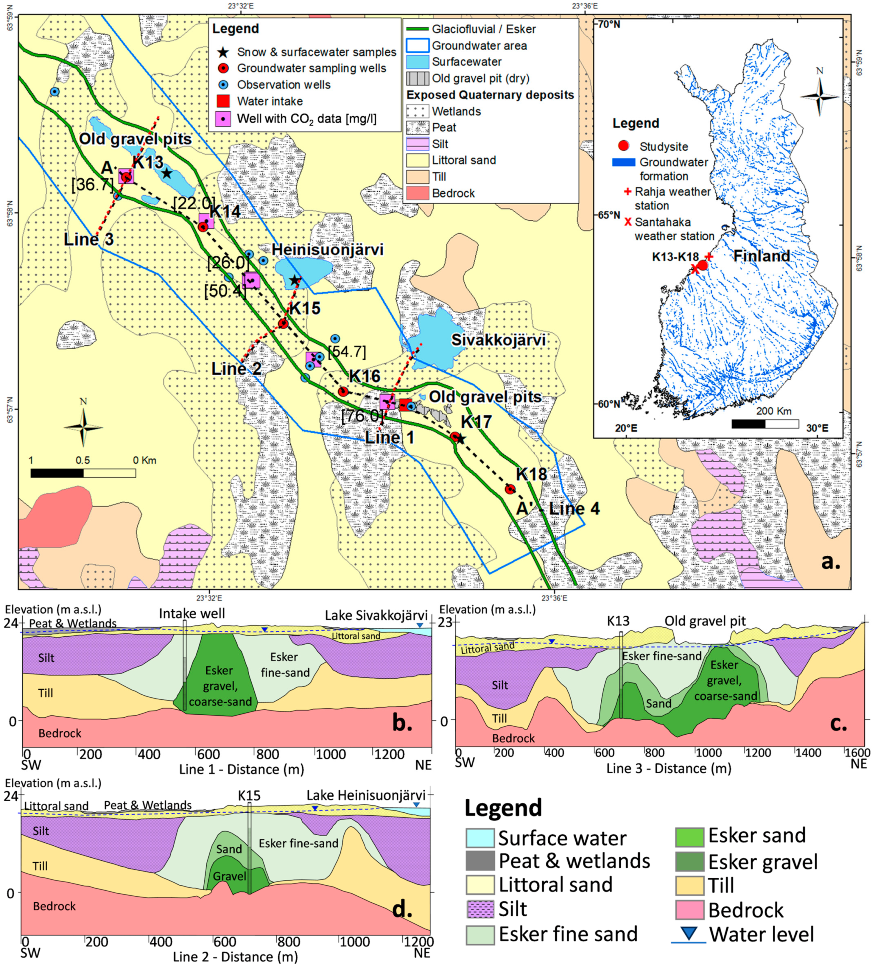
In this study, we characterized the geochemistry of groundwater in an unconfined esker aquifer in western Finland. The factors and processes controlling the geochemistry of the groundwater were identified based on a three-year seasonal data set collected during 2010–2013. Previous studies on groundwater quality in Finland have mainly provided snapshots, and water samples have been collected from one well per aquifer, which may not represent either the spatial or temporal variability in groundwater chemistry. Here, we aimed to demonstrate in a sub-Arctic cold environment that spatial, temporal, and seasonal variations in groundwater chemistry are clearly visible within the aquifer. We also aimed to demonstrate that seasonality (climate variability) affects the results in such a shallow unconfined esker aquifer.

2. Study Area

2.1. General Setting

The study area is located in western Finland (Figure 1) and covers an area of approximately 10 km². The Karhinkangas aquifer is an unconfined esker aquifer consisting of sand and gravel. It is classified as an important groundwater area for water supply [26], and the groundwater recharge rate is on average 12,700 m³/d [11]. There is a water intake plant in the area, having one intake well, where the average pumping rate has been 60 m³/d (Figure 1). However, the number of intake wells will increase, and the pumping rate is expected to increase to 10,000 m³/d to supply sufficient water for the municipality and local industry. The topography varies between 0 and 27 m a.s.l., and the land surface elevation decreases from the mainland to the northern coast of the Bothnia Sea (Figure 1). The Karhinkangas area is in the cold and humid climate zone, with the mean annual precipitation and temperature during 1981–2010 being 712.4 mm and +6 °C, respectively [27]. The lowest daily temperatures are generally recorded in January and February (with an average of −0.6 °C), and the highest during July and August (with an average of +14.8 °C).

2.2. Geological and Hydrogeological Background

The bedrock in the study area mainly consists of Precambrian crystalline bedrock, e.g., granodiorite, biotite-rich paragneiss and paraschist, granite, and a small proportion of graphite sulfide paraschist [28], overlain by Quaternary deposits, including till, glaciofluvial sand and gravel, marine and lacustrine clays and silts, littoral sediments, and peat (Figure 1), which were deposited during the Weichselian and Holocene deglaciation of the Scandinavian Ice Sheet [2,29]. The Karhinkangas aquifer belongs to the interlobate esker complex of porous sand and gravel, which runs in a NW–SE direction from the mainland in the south to the Bothnian Sea in the north. Figure 1b–d illustrate geological cross-sections of the Quaternary deposits and surface water along lines 1–3 (Figure 1), which were built based on the interpretation of the GPR profiles as described in [11]. The aquifer is unconfined, and the average soil thickness is approximately 20 m. The groundwater table in the study area follows the topography and decreases almost linearly from 23 m a.s.l. inland to 0 m a.s.l. on the Baltic Sea coast. Based on the results of pumping tests and soil sample analysis, the hydraulic conductivity of the aquifer varies from 1.67 × 10⁻⁵ to 2.31 × 10⁻³ m/s from sand to gravel, respectively [11].

Groundwater recharge occurs twice a year during spring (April) and late autumn (November to December) due to spring snowmelt and rainfall, respectively. In summer, the evapotranspiration rate is high, and the groundwater table decreases. Groundwater flows northwest towards the coastal area and discharges into low-lying areas consisting of peatlands and wetlands. In the study area, two small lakes (Lakes Sivakkojärvi and Heinisuonjärvi) exist in the east and in a gravel excavation pit adjacent to observation borehole K13, where some parts of the old pits have filled with water (Figure 1). Another small old gravel pit is located near borehole K17. This pit is dry, but the removed soil has reduced the unsaturated soil thickness, with the average groundwater table being less than 0.5 m below the ground surface.

3. Materials and Methods

The data used in this study were collected in a field investigation and consist of drill borehole data, as well as ground-penetrating radar, seismic refraction, and gravity measurement data reported in [11]. Groundwater sampling for geochemical analysis was collected quarterly from autumn 2010 to autumn 2013 (no sampling was performed in autumn 2011) and was carried out in two parts: (1) the regional study; and (2) the site-specific study with the monitoring of groundwater geochemistry in this study area. The regional groundwater geochemistry from autumn 2010 (6 to 12 October 2010) revealed variability in redox zones and elevated Fe and Mn concentrations. The monitoring of groundwater geochemistry was then carried out from six observation boreholes (K13–K18) covering the high variation in the redox zone (Figure 2) from winter 2011 to autumn 2013. The sampling was conducted according to the groundwater level (i.e., seasonal sampling) during periods of high and low groundwater. In addition, three snow samples were taken next to K17 and analyzed during winter 2011 and winter and spring 2012. The methods used consisted of the integration of geochemical analysis utilizing the Piper diagram, which is a plot of the relative concentrations of major dissolved species of anions and cations [30], by using the program GW_Chart [31], and multivariate statistical analysis (principal component analysis (PCA) and hierarchical cluster analysis (HCA)). Details of the data and methods applied are presented in the sections below.

3.1. Groundwater and Snow Sampling and Analysis

The field investigation consisted of down-hole water profile logging and field measurement of water samples. The profile logging was performed to investigate the vertical distribution of physical and chemical parameters in groundwater at the screen intervals of the observation wells, and the sampling depths in profiled water sampling were selected based on the results of these logs. Measurements were performed by using a YSI Professional Plus (IP-67) multi-parameter recording device for the measurement of pH, electrical conductivity (EC), dissolved oxygen (DO), and temperature. However, alkalinity was measured by using automatic potentiometric titration immediately upon arrival of the samples at the laboratory. Before the profile logging and the water sampling were performed, groundwater from the observation boreholes was pumped out until the water parameter readings (e.g., temperature, EC) were constant. For the profile sampling, the partition samples were taken by placing an inflatable packer at the discrete depth of the selected zones (Figure 2), and a single groundwater sample was collected at a time at a low pumping rate (approximately at rate of 0.5 L/min) to minimize the disturbance of water across the sampling interval. The samples were initially taken from the top section and continued downwards to the bottom section.

A total of 181 groundwater samples consisted of 143 profiled samples from three observation boreholes (K13, K14, and K17) (Figure 2). Three profiled samples were taken from borehole K15 (K151, K152, and K153) in autumn 2010, while the rest of the samplings representing the whole screen interval were taken from K152, K16, and K18 (total 38 samples).

In addition to the water sampling campaign in 2010–2013, the geochemistry of surface water samples taken by [32] from Lakes Sivakkojärvi and Heinisuonjärvi on 5 June and 15 July 2019, and by [33] from Lake Heinisuonjärvi on 20 May 2015, as well as the concentrations of dissolved carbon dioxide gas (CO₂) and total organic carbon (TOC) in groundwater measured in 2011 by [11] from six observation boreholes as shown in Figure 1, were used to support the interpretation.

In this paper, for example, K13 refers to observation borehole 13, K131 denotes sample 1 taken from K13 (Figure 2), and K131/1 to K131/12 represent sample 1 from K13 taken from data sets 1 (autumn 2010, first data set) to 12 (autumn 2013, final data set). The abbreviations w, sp, s, and a denote the seasons winter (March), spring (May), summer (August), and autumn (November), respectively (Figure 3).

For cation analysis, water samples were filtered through 0.45 µm membrane filters and collected into 100 mL high-density polyethylene (HDPE) bottles. The samples were acidified with 0.5 mL HNO₃/100 mL water (to prevent the precipitation of metals) and analyzed in the accredited laboratory of Labtium Ltd in Espoo. Filtered and acidified water samples were analyzed for major and minor elements (Ag, Al, As, B, Ba, Be, Bi, Cd, Co, Cr, Cu, I, K, Li, Mn, Mo, Ni, P, Pb, Rb, Sb, Se, Sr, Th, Tl, U, V, Ca, Fe, Mg, Na, Si, Zn, and S) using inductively coupled plasma atomic emission and mass spectrometry (ICP-AES and ICP-MS). Alkalinity (as HCO₃), EC, pH, and KMnO₄ consumption were measured from unfiltered and unpreserved samples immediately upon arrival of the samples at the laboratory. The samples were also analyzed for anions (Br, Cl, F, NO₃, PO₄, and SO₄) and NH₄ using an ion chromatography (IC) technique. Total dissolved solids (TDS) were calculated from the sum of all dissolved concentrations for each water sample. At each sampling season, one blank sample was prepared from distilled water and one duplicated groundwater sample was analyzed. The analytical error for measured parameters varies from 3 to 15%. Analytical results for blank and duplicate samples indicated no field contamination. The charge balance error (CBE) and the concentration of dissolved CO₂ gas were calculated by using PHREEQC Interactive version 3.3.9 [34] with the wateqf4.dat thermodynamic database [35] for all samples. According to the results, 172 samples had CBE values less than ±5%, while 9 samples had CBE values between ±5% and ±10%. Appelo and Postma [36] recommended a CBE cutoff of less than ±5% for good water analysis, while [37,38] used a CBE cutoff of ±10% due to the presence of high organic acid concentrations in groundwater samples. In this study, the CBE cutoff of ±10% was applied and all water samples were included in the analysis.

The groundwater table and temperature were monitored hourly at all observation wells during the same period. The measurement was performed by installing a Solinst LeveloggerTM Model 3001 data logger and pressure transducer at the bottom of each observation well. Daily climate data (air temperature and precipitation) in the same period were obtained from the Santahaka–Kokkola weather station (approximately 30 km southwest of the study area) [27]. Microsoft Excel was used for data storage and performing basic calculations. Interpolation of geochemical and profile logging data was performed in ArcGIS/ArcMap version 10.8.2.

3.2. Stable Isotopic Composition of Oxygen and Hydrogen

The stable isotopic composition of oxygen (δ¹⁸O) and hydrogen (δD) was used to identify the source of groundwater and the degree of groundwater and surface water interactions from the mixing processes of isotopically distinct water masses and evaporation in surface water reservoirs [13,39,40]. Water samples for the stable isotope analysis consisted of 124 groundwater samples taken from the six observation boreholes (K13–K18) during 2011–2013, three snow samples taken at the site of K17 during the winters of 2011, 2012, and 2013, and four surface water samples taken during summer 2016 from Lakes Sivakkojärvi and Heinisuonjärvi and a pond in an old gravel pit (close to K13) (Figure 1). For analysis of the stable isotopes δ¹⁸O and δD, non-filtered samples were taken into 60 mL HDPE bottles, sealed, and kept in a dark cooler box while being transported to the Research Laboratory of the Geological Survey of Finland in Espoo. The isotopic composition of δ¹⁸O and δD was analyzed by laser-based cavity ring-down spectroscopy (CRDS) using a Picarro isotopic water analyzer. In the CRDS method, the absolute abundances of water molecules with different combinations of the stable isotopes of δ¹⁸O and δD are measured from a vaporized sample in an optic chamber. The isotopic composition of water is reported using the δ notation per mill (‰) relative to the Vienna Standard Mean Ocean Water (VSMOW). The repeatability of analyses was <0.1‰ (1 σ) for δ¹⁸O and 0.5‰ for δD. Deuterium excess (d-excess) was calculated as an index of the evaporation effect for each water sample using the following equation [41]:

d-excess = δD – 8δ¹⁸O

(1)

3.3. Statistical Analysis

Statistical analysis was performed using IBM SPSS statistical software version 28 [42] to determine the variables that represent the controlling factors behind the geochemistry of all the water samples. Two multivariate statistical approaches, principal component analysis (PCA) and hierarchical cluster analysis (HCA), were used to group the water samples or variables.

PCA is a factor analysis method that is used to extract components representing the information contained in the data that explain the pattern of correlations and differences within a group of variables [42,43]. The number of factors or components was extracted by PCA with varimax rotation based on Kaiser normalization. Although PCA measures the variance of the data set using the eigenvector technique, which is applied in the space domain, by applying PCA to the normalized time series data, the principal component loadings should be able to identify the similarity of the variables, and consequently reveal the processes and factors controlling the geochemistry of groundwater [8,13,16].

HCA is a classification method that reveals natural groupings or clusters within a data set by reorganizing the data into homogeneous groups and linking the two most similar clusters until all the variables are joined in a complete classification tree [42,43]. The results of HCA are presented in a dendrogram, which is constructed using Ward’s method [44] with the Euclidean distance as a measure of similarity between the samples. Ward’s method is one of the most widespread hierarchical clustering methods for the classification of hydrogeochemical data by using the minimum variance to evaluate the distances between the clusters [13,45,46,47].

The data used for PCA and HCA comprised of the chemical parameters, pH, DO, CO₂, EC, and temperature. In the case of values below the detection limit (DL), the value of DL/2 was used for the analysis [48]. All parameters were examined for deviations from a normal distribution by using the P–P (probability–probability) plot [42]. The data set includes variables having normal or close to normal distributions from the chemical parameters (Ba, K, Mg, Na, Cl, Si, SO₄, CO₂(g), temperature, pH, alkalinity (as HCO₃)). The variables with a non-normal distribution (Al, As, Ca, Fe, Mn, PO₄, Co, Cr, Cu, Ni, Zn, EC, DO, and KMnO₄ consumption) were log-transformed prior to statistical analysis. The variables with non-normal distribution (B, Li, Rb, U, and V) and more than 45–95% of values below or close to the detection limit (Ag, Be, Bi, Cd, I, Pb, Sb, Se, Th, Tl, Br, F, NO₃, and NH₄) were excluded from the analysis. The valid data were standardized by subtracting the sample mean from each variable and dividing the resulting value by the standard deviation (Z-score standardization) prior to multivariate analysis to ensure that each variable was weighted equally.

4. Results

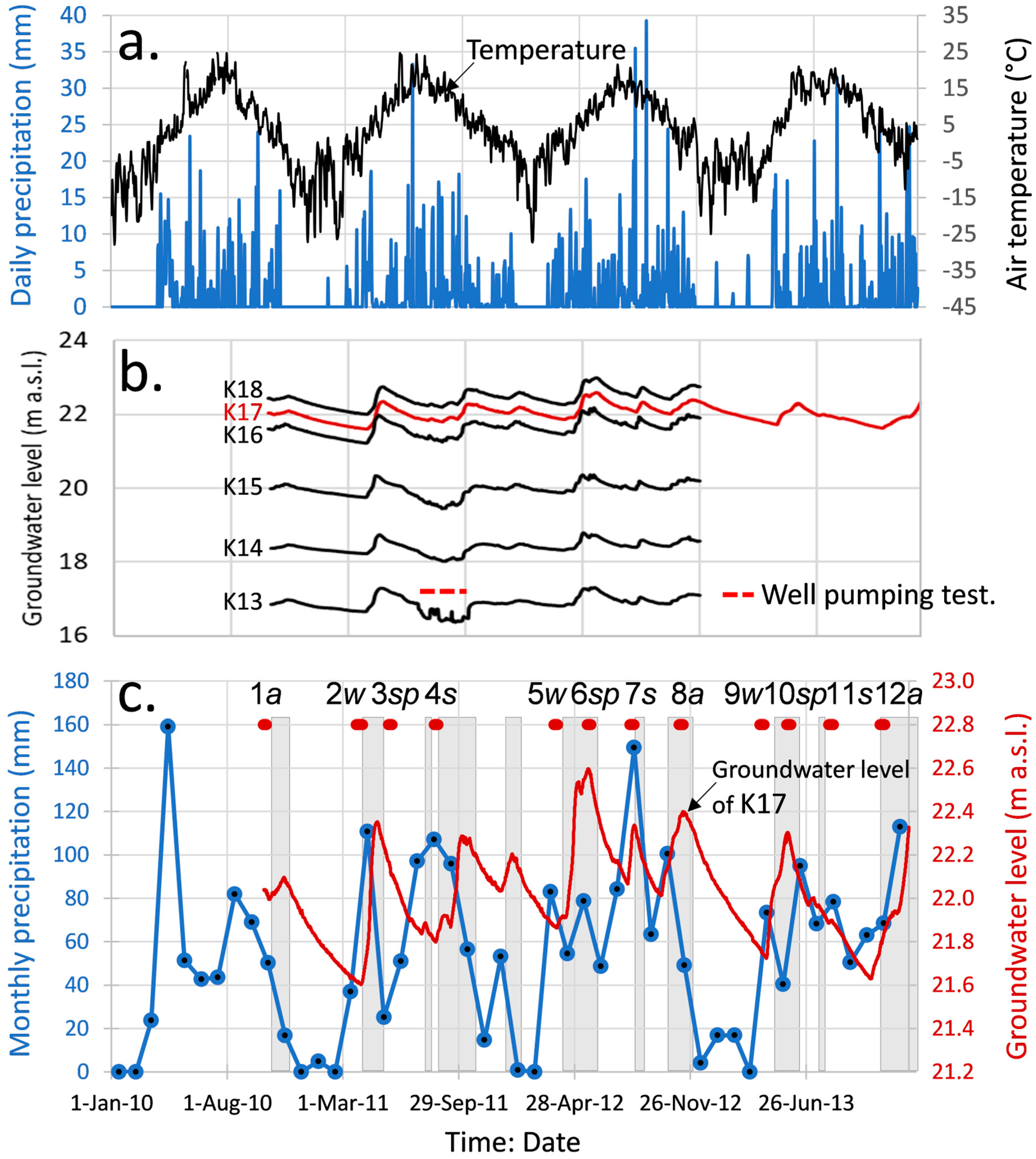
4.1. Groundwater Level

Figure 3 presents the groundwater levels recorded from K13 to K18, the groundwater sampling periods, daily temperature, daily precipitation, and monthly precipitation from the Santahaka–Kokkola weather station [27] from January 2010 to December 2013. The variations in the groundwater level indicated two groundwater recharge periods (Figure 3c): during spring (early May), immediately after the snowmelt period, and during late autumn (October to December), when evapotranspiration is low and there is no snow cover. Groundwater reached the lowest levels during the winter and late summer due to snow cover and evapotranspiration, respectively. From 2010 to 2013, the mean groundwater level varied between 17 m a.s.l. in K13 and 23 m a.s.l. in K18 (approximately 0.9–3.9 m b.g.s.), and the average horizontal hydraulic gradient between these wells was 0.0012.

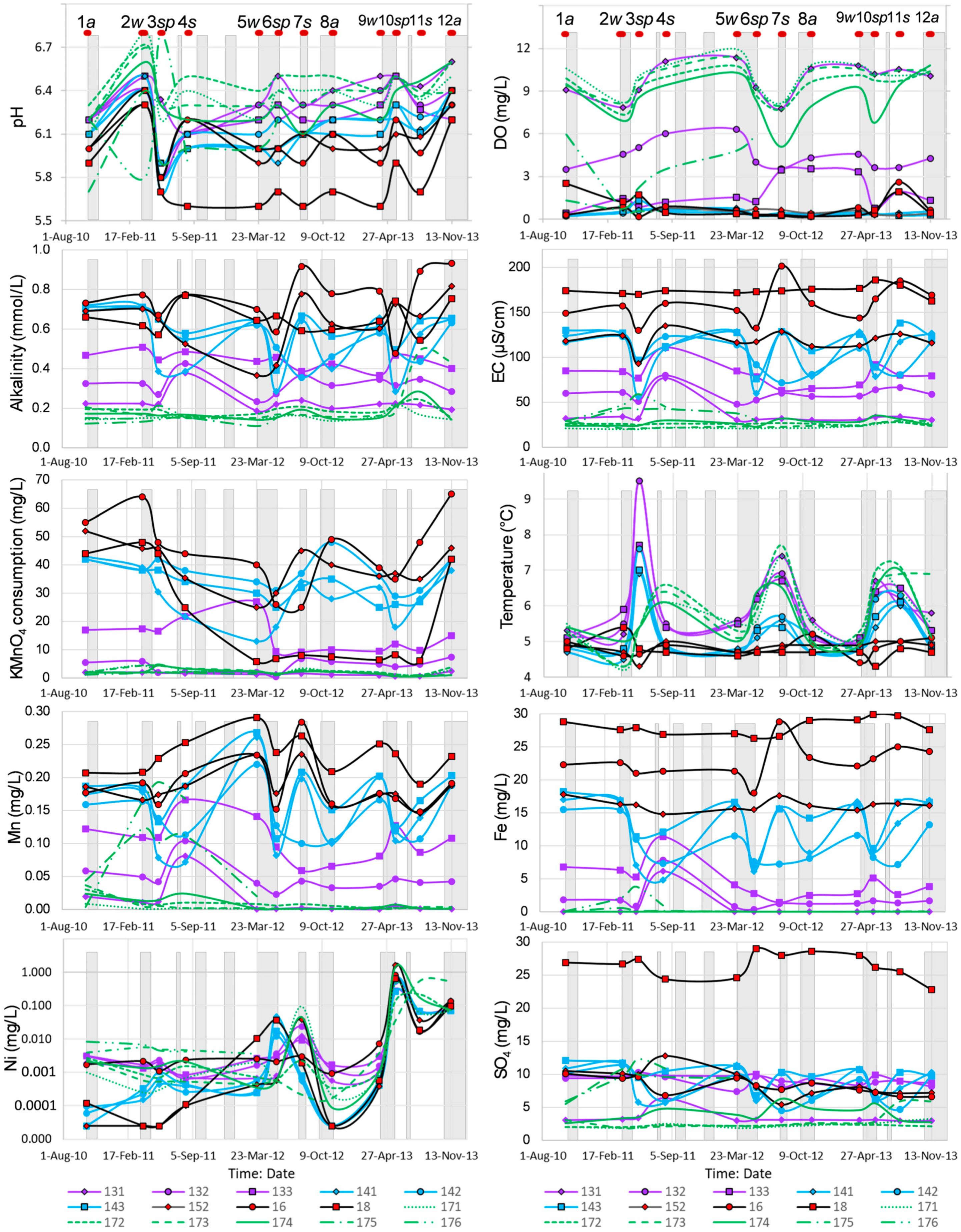
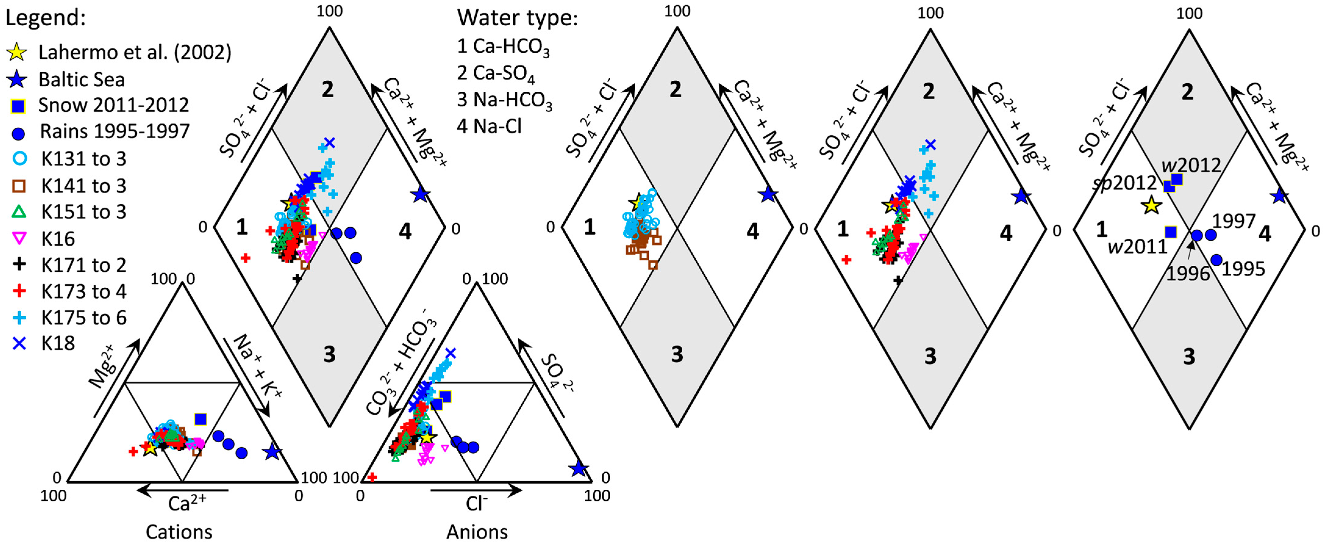
4.2. Hydrogeochemistry

Table 1. Characteristics of groundwater (mean, median, min, max) in the Karhinkangas area (number of samples, n = 181), the median values for groundwater in each season, and the suggested limit values or range of drinking water values based on [52]. Values that exceed the drinking water limit are bolded. For the seasonal data, the values that are higher than the previous data set are highlighted with a gray background.

Variable	Unit	Min.	Median	Mean	Max.	Winter	Spring	Summer	Autumn	Drinking
n		181				45	45	44	47	Water
Temp.	°C	4.20	5.30	5.52	9.50	4.90	6.10	6.10	5.10
DO	mg/L	0.17	2.21	4.53	13.01	3.31	2.21	2.06	2.50	5.00
pH		5.60	6.28	6.23	6.80	6.30	6.20	6.20	6.20	6.50–9.50
EC	µS/cm	20.00	59.90	73.92	201.40	57.00	52.40	69.05	60.00	2500.00
TDS	mg/L	28.47	57.75	78.79	193.14	57.05	50.81	67.27	57.71
CO2	mg/L	3.36	23.40	29.90	82.43	18.77	22.90	28.15	23.00
Alkalinity	mmol/L	0.11	0.32	0.37	0.92	0.33	0.27	0.36	0.33
K	mg/L	0.58	1.23	1.24	2.44	1.34	1.18	1.23	1.21
Ca	mg/L	1.43	3.99	4.06	8.16	4.03	3.16	4.32	4.31
Mg	mg/L	0.43	1.26	1.29	2.70	1.57	0.96	1.23	1.50
Na	mg/L	0.88	2.77	3.17	11.00	2.76	2.56	3.17	3.04	200.00
Cl	mg/L	0.41	1.60	2.13	12.00	1.50	1.40	1.78	1.73	250.00
Si	mg/L	4.61	6.92	7.11	11.30	7.08	6.79	6.97	6.59
SO4	mg/L	0.59	6.80	7.58	29.00	8.33	6.20	6.10	7.15	250.00
Fe	mg/L	<0.03	1.75	7.59	29.90	1.75	0.97	2.03	2.07	0.20
NO3	mg/L	<0.20	<0.20	<0.20	1.30	<0.20	<0.20	<0.20	<0.20	50.00
NH4	mg/L	<0.05	<0.05	<0.05	0.43	<0.05	<0.05	<0.05	<0.05	0.50
PO4	mg/L	<0.02	<0.02	0.09	0.47	<0.02	<0.02	<0.02	<0.02
KMnO4	mg/L	0.44	5.50	16.18	65.00	4.90	4.40	5.45	7.40	20.00
Mn	µg/L	0.38	78.50	90.76	291.00	80.90	78.50	76.45	65.60	50.00
Ba	µg/L	3.01	17.10	23.86	91.10	17.70	15.80	17.25	16.20
Al	µg/L	1.60	34.50	76.98	1280.00	16.00	43.70	41.15	45.20	200.00
As	µg/L	<0.05	0.21	0.29	1.57	0.19	0.22	0.29	0.22	10.00
Co	µg/L	<0.02	0.20	0.51	3.63	0.15	0.30	0.27	0.14
Cr	µg/L	<0.20	1.25	2.30	11.60	0.63	2.17	1.65	1.12	25.00
Cu	µg/L	<0.10	0.23	0.44	3.84	0.46	0.32	0.18	0.18	2000.00
Ni	µg/L	<0.05	1.72	66.53	1660.00	0.87	3.64	7.03	1.74	20.00
Zn	µg/L	<0.20	2.36	2.86	12.10	2.02	2.90	2.19	2.21

presents a statistical summary of the groundwater chemistry in Karhinkangas and

Table 2. The median values of groundwater variables in the Karhinkangas area for all water samples (GW) and for all seasons compared with data on the median values for shallow groundwater in Finland (Finland) from [17]; snow samples taken during winter 2011, winter 2012, and spring 2012 (Snow); rainfall data (Rain) from [49,50,51], and surface water from Lakes Sivakkojärvi (Sivakjv) and Heinisuonjärvi (Heinisjv) taken during 20 May 2015, 5 June 2019, and 15 July 2019 from [32,33]. Values that are higher than the median values in Finland are bolded. For the seasonal data, values that are higher than the previous data set are highlighted with a gray background.

Variable	Unit	GW	Winter	Spring	Summer	Autumn	Finland	Snow	Rain	Sivakjv.	Heinisjv.
n		181	45	45	44	47	739	3	31	2	3
Temp.	°C	5.30	4.90	6.10	6.10	5.10	6.80
DO	mg/L	2.21	3.31	2.21	2.06	2.50	7.40			8.57	9.83
pH		6.28	6.30	6.20	6.20	6.20	6.40	5.00	4.92	6.24	7.24
EC	µS/cm	59.90	57.00	52.40	69.05	60.00	125.00		17.45	22.70	33.00
TDS	mg/L	57.75	57.05	50.81	67.27	57.71		20.67
CO2	mg/L	23.40	18.77	22.90	28.15	23.00	34.00
Alkalinity	mmol/L	0.32	0.33	0.27	0.36	0.33	0.55	0.07	0.03
K	mg/L	1.23	1.34	1.18	1.23	1.21	2.78	0.93	0.44
Ca	mg/L	3.99	4.03	3.16	4.32	4.31	11.40	2.74	0.24
Mg	mg/L	1.26	1.57	0.96	1.23	1.50	2.38	0.71	0.13
Na	mg/L	2.77	2.76	2.56	3.17	3.04	4.18	0.71	0.44
Cl	mg/L	1.60	1.50	1.40	1.78	1.73	4.46	0.80	0.80		1.10
Si	mg/L	6.92	7.08	6.79	6.97	6.59	12.90	5.23
SO4	mg/L	6.80	8.33	6.20	6.10	7.15	10.40	3.00	0.60		3.20
Fe	mg/L	1.75	1.75	0.97	2.03	2.07	<0.03	<0.03			1.48
NO3	mg/L	<0.20	<0.20	<0.20	<0.20	<0.20	3.19	1.10	0.32	<2.00	<2.00
NH4	mg/L	<0.05	<0.05	<0.05	<0.05	<0.05		0.14	0.32	<0.03	<0.03
PO4	mg/L	<0.02	<0.02	<0.02	<0.02	<0.02	<0.02	<0.02	0.03	0.16	0.12
KMnO4	mg/L	5.50	4.90	4.40	5.45	7.40	4.50
Mn	µg/L	78.50	80.90	78.50	76.45	65.60	4.36	2.45			3.00
Ba	µg/L	17.10	17.70	15.80	17.25	16.20	18.10	5.43
Al	µg/L	34.50	16.00	43.70	41.15	45.20	101.00	4.94			150.00
As	µg/L	0.21	0.19	0.22	0.29	0.22	0.14	0.11		<1.00	<1.00
Co	µg/L	0.20	0.15	0.30	0.27	0.14	0.09	0.22		<0.50	<0.50
Cr	µg/L	1.25	0.63	2.17	1.65	1.12	0.20	0.25		0.83	0.63
Cu	µg/L	0.23	0.46	0.32	0.18	0.18	2.49	0.24		<1.00	<1.00
Ni	µg/L	1.72	0.87	3.64	7.03	1.74	0.84	1.06		<3.00	<3.00
Zn	µg/L	2.36	2.02	2.90	2.19	2.21	10.40	3.13		27.60	18.30

presents the median values for the groundwater, snow, and surface water (Lakes Sivakkojärvi and Heinasuonjärvi) chemistry of Karhinkangas, the shallow groundwater in Finland from [17], and rainwater collected from the Rahja weather station in Kalajoki, approximately 25 km northeast of the study area, from [49,50,51]. Snow and rainfall contained low values of TDS (20.67 mg/L), EC (17.45 µS/cm), pH (4.92–5.00), and alkalinity (0.03–0.07 mmol/L) (Table 2). Overall, groundwater contained low values of TDS (28.47–193.14 mg/L), EC (20.00–201.40 µS/cm), pH (5.60–6.80), and alkalinity (0.11–0.92 mmol/L) (Table 1). The median concentrations of major ions in the groundwater were lower than the median values reported for Finnish shallow groundwater by [17], except for the median values of Fe, Mn, KMnO₄ consumption, As, Co, Cr, and Ni. In particular, the elevated concentrations of dissolved Fe and Mn exceeded the drinking water limits [52]. Groundwater geochemistry displayed seasonal variation, with the lowest DO values and the highest TDS, EC, CO₂, and concentrations of major ions and Fe during summer (Table 1). However, the median concentrations of K, Mg, Si, SO₄, Ba, and Mn were highest during winter. During spring, when the groundwater table was at the highest level due to snow melt, the EC value and the concentrations of ions and Fe were lowest.

Figure 4 illustrates the variability in pH, DO, alkalinity, EC, KMnO₄ consumption, temperature, and concentrations of Mn, Fe, Ni, and SO₄ in groundwater samples from autumn 2010 to autumn 2013. Figure 5 presents the longitudinal sections (north–south direction), showing the interpolated values of pH, DO, EC, temperature, KMnO₄ consumption, alkalinity, concentrations of major ions (Ca, Mg, K, Na, Cl, SO₄), Fe, and Mn, and d-excess of groundwater samples in spring 2011. The groundwater profile revealed distinct oxidizing and reducing zones. The oxidizing zone contained >0.5 mg/L DO and was mainly evident in shallow water samples, such as in K131, K132, K171, K172, K173, and K174. Borehole K13 is located in sand and gravel deposits near the gravel excavation pits (Figure 1), while K17 is located in the esker ridge forest area, where the main aquifer materials consist of sand and fine sand (Figure 2). The reducing zone was detected in the deeper part of the aquifer, such as in samples K133, K175, and K176. The DO concentrations in K14, K15, and K16 were found to be low from the upper part down to the bottom of the boreholes (Figure 5). These boreholes are located in the sand and gravel of the esker core area (i.e., the center of the esker formation), which is close to the ground surface (Figure 2) and covered by peat and wetlands with a high organic matter content. Except for DO, the dissolved solute concentrations, EC, KMnO₄ consumption, and CO₂ concentration were higher in the reducing zone than in the oxidizing zone (Table 4). The CO₂ concentrations presented in Table 1, Table 2, and Table 4 were obtained from PHREEQC calculation. These CO₂ concentrations are in alignment with the measured CO₂ data from [11], which varied between 22.0 and 36.7 mg/L in the oxidizing zone and up to 76 mg/L in the reducing zone (Figure 1a), similarly to TOC, which varied between 7.2 and 8.3 mg/L and 45 and 58 mg/L in the oxidizing and reducing zones (Figure not shown), respectively. The concentrations of ammonium (NH₄) and phosphate (PO₄) were low and displayed the same patterns as the other parameters, with higher concentrations in the reducing zone and values below the detection limit in the oxidizing zone (Table 1, Figures not shown). Most of the nitrate (NO₃) concentrations were below the detection limit, except for K141, where three samples from spring 2011, spring 2012, and autumn 2012 contained NO₃ concentrations of 0.38, 1.30, and 0.41 mg/L, respectively. Water sampled from K18 contained the highest concentrations of dissolved Fe, Mn, and SO₄ and the lowest pH value (pH 5.60) compared to the other samples. The DO concentrations in K18 varied between 0.20 and 2.50 mg/L (Figure 4).

The groundwater in the Karhinkangas aquifer was found to be mainly of the Ca-HCO₃ type, except for the water samples from K18, K175, and K176, which were more of the Ca-HCO₃-SO₄ type (Figure 6). These samples contained higher dissolved sulfate concentrations compared to the others (Figure 4). The snow samples taken from K17 were of the same water type as the groundwater. Due to the short distance from the seashore, rainwater samples taken from the Rahja weather station, approximately 25 km northeast of the study area [49,50,51], were of the Na-Cl type. Groundwater samples in this study displayed no evidence of saltwater intrusion.

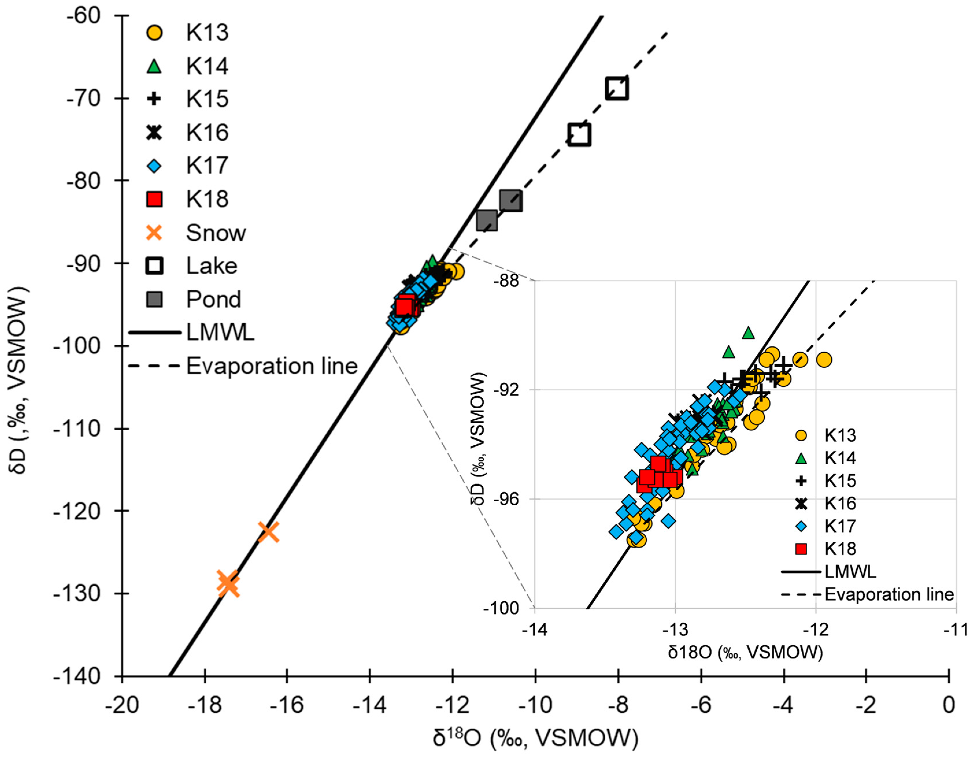
4.3. Stable Isotopes of Oxygen and Hydrogen

The stable isotopes δ¹⁸O and δD and d-excess values of the water samples are summarized in

Table 3. A statistical summary of the values for the stable isotopes δ¹⁸O and δD and d-excess in the water samples. All values are reported as per mil.

Variable	Min.	Median	Mean	Max.
Surface water (lakes and pond), (n = 4)
δD	−84.70	−71.50	−78.48	−68.70
δ18O	−11.18	−8.50	−9.88	−8.05
d-excess	−4.30	−3.50	0.56	4.74
Snow (n = 3)
δD	−129.20	−128.40	−126.70	−122.50
δ18O	−17.44	−17.41	−17.10	−16.46
d-excess	9.18	10.08	10.13	11.12
Groundwater (n = 124)
δD	−97.50	−93.50	−93.71	−89.90
δ18O	−13.31	−12.81	−12.82	−11.94
d-excess	4.60	9.00	8.85	11.70

. Figure 7 presents a plot of δ¹⁸O versus δD in the groundwater, snow, and surface water (lakes and pond) samples. The local meteoric water line (δD = 7.67 δ¹⁸O + 5.79‰ [53]) and the local evaporation line were plotted for comparison. There were differences in the stable isotope composition between the groundwater and surface water samples (Figure 7). All groundwater samples, except K13 and K15, were situated on the local Finnish meteoric water line, while groundwater samples from K13 and K15 were situated on the evaporation line with the surface water samples.

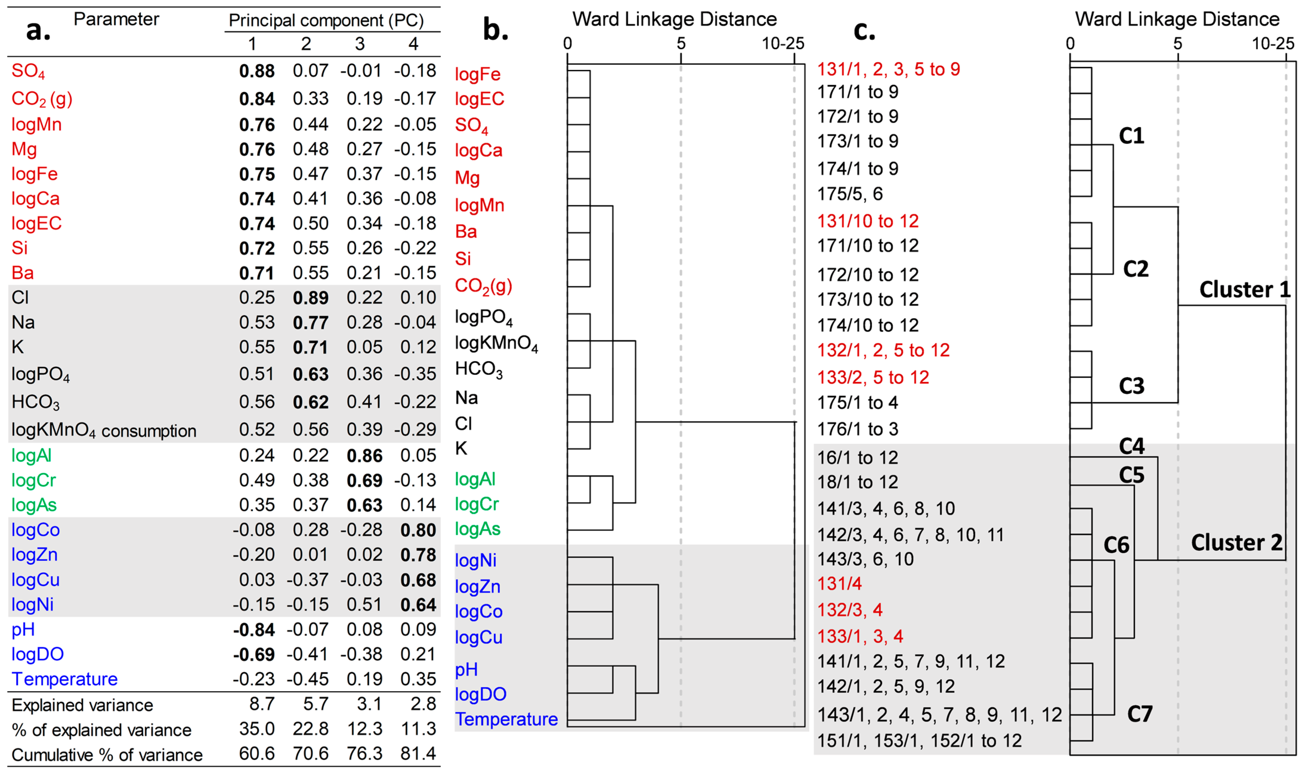
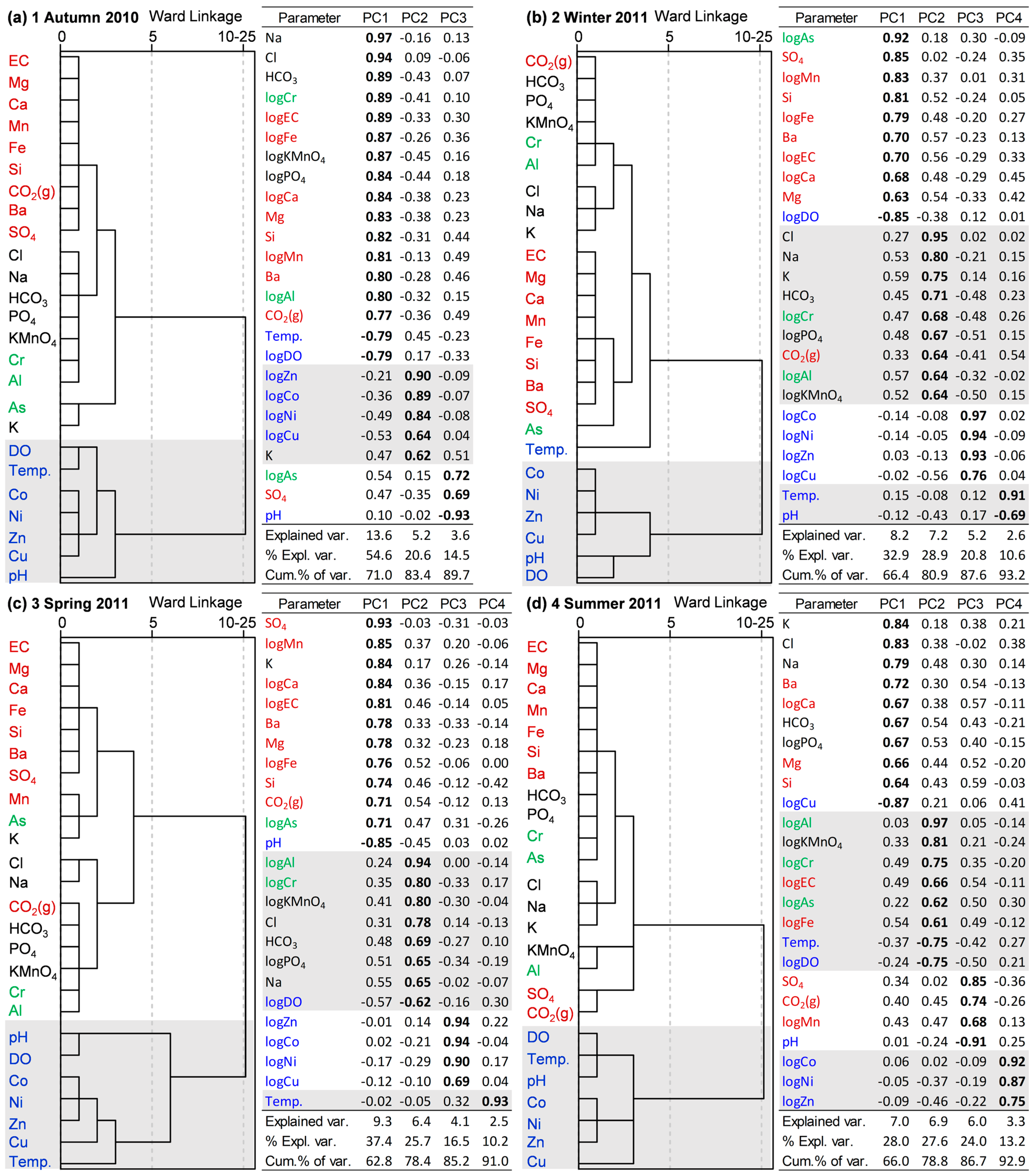
4.4. Principal Component Analysis (PCA) and Hierarchical Cluster Analysis (HCA)

Figure 8 presents a panel of the PC loadings from principal component analysis and the explained variances of geochemical variables for all groundwater samples from autumn 2010 to autumn 2013 (n = 181) (8a), as well as the hierarchical clustering results (dendrogram) for water samples based on both variables (8b) and locations (sampling depth/sampling period) (8c). For all groundwater samples, all variables (K, Mg, Na, Cl, SO₄, HCO₃, Si, Ba, CO₂(g), pH, temperature, logDO, logEC, logCa, logFe, logMn, logPO₄, logAl, logAs, logCo, logCr, logCu, logNi, logZn, logKMnO₄ consumption) were classified into the four main principal components (PC) with eigenvalues > 1, explaining over 81.4% of the total variance observed.

PC1 explained 35.0% of the variance and has strong positive loadings for SO₄, CO₂(g), Mn, Mg, Fe, Ca, EC, Si, and Ba, and negative loadings for pH and DO. KMnO₄ consumption has similar positive loadings of 0.52 and 0.56 for PC1 and PC2, respectively.

PC2 explained 22.8% of the variance and has high positive loadings for Cl, Na, K, PO₄, and HCO₃.

PC3 explained 12.3% the variance and has high positive loadings for Al, Cr, and As.

PC4 explained 11.3% the variance and has high positive loadings for trace metals (Co, Zn, Cu, and Ni).

Temperature has a poor negative loading for PC1 and PC2 and a poor positive loading for PC3 and PC4. The PC classification is similar to the sub-clusters of HCA, as illustrated in Figure 8b.

The groundwater samples were clustered into hierarchical clusters (Ward’s method) based on the linkage distance in the dendrogram, indicating the level of similarity of variables between the clusters. The shorter the linkage distance, the higher the similarity of variables between clusters. For all groundwater samples, the water was classified into two main clusters based on the linkage distance at 25 for both variable and location categories, as illustrated in Figure 8b and Figure 8c, respectively. Based on the locations of the samples (Figure 8c), the median values of variables in each HCA sub-cluster are presented in

Table 4. Median values of variables in the HCA sub-clusters from groundwater samples (n = 181) taken from autumn 2010 to autumn 2013. Lists of samples in each cluster are presented in Figure 8c. The minimum values are highlighted with a gray background and the maximum values with a gray background and bolding.

HCA Cluster	1 (Oxidizing Zone)			2 (Reducing Zone)
Sub-Cluster	1	2	3	4	5	6	7
Number of samples (n)	54	21	26	12	12	22	34
Temperature (°C)	5.45	6.40	5.50	4.80	4.70	5.45	4.80
DO (mg/L)	9.46	10.20	3.37	0.47	0.45	0.39	0.42
pH	6.37	6.50	6.30	6.00	5.70	6.10	6.10
EC (µS/cm)	26.00	27.70	60.05	158.40	173.35	80.80	123.65
TDS (mg/L)	35.85	39.04	57.34	160.92	135.32	88.57	126.82
CO2 (mg/L)	9.99	7.16	20.69	57.85	51.67	39.57	53.93
Alkalinity (mmol/L)	0.17	0.20	0.33	0.77	0.64	0.44	0.65
K (mg/L)	0.89	0.91	1.38	2.13	1.56	1.19	1.50
Ca (mg/L)	1.94	2.49	4.37	5.70	7.47	4.37	6.03
Mg (mg/L)	0.58	0.59	1.58	2.04	2.35	1.49	1.95
Na (mg/L)	1.41	1.38	2.75	8.02	4.71	3.82	4.58
Cl (mg/L)	0.75	0.71	1.69	8.28	1.81	2.18	3.18
Si (mg/L)	5.38	5.20	6.70	9.81	9.78	7.68	8.95
SO4 (mg/L)	2.58	2.90	9.39	8.00	26.80	6.57	10.15
Fe (mg/L)	<0.03	<0.03	1.67	22.45	27.75	7.47	16.15
NO3 (mg/L)	<0.20	<0.20	<0.20	<0.20	<0.20	<0.20	<0.20
NH4 (mg/L)	<0.05	<0.05	<0.05	0.15	<0.05	<0.05	0.08
PO4 (mg/L)	<0.02	<0.02	<0.02	0.39	<0.02	<0.02	0.20
KMnO4 (mg/L)	2.00	1.00	5.65	46.00	8.10	27.00	36.50
Mn (µg/L)	2.20	1.59	73.25	176.50	234.00	107.00	185.00
Ba (µg/L)	4.61	6.19	16.10	65.10	72.15	23.25	39.75
Al (µg/L)	10.00	50.70	21.25	85.60	25.65	143.00	91.60
As (µg/L)	0.09	0.15	0.19	0.64	0.47	0.42	0.29
Co (µg/L)	0.19	0.20	1.03	1.83	0.03	0.28	0.04
Cr (µg/L)	0.15	0.62	0.91	5.28	3.55	3.48	4.11
Cu (µg/L)	0.22	0.24	1.09	<0.10	<0.10	0.40	0.05
Ni (µg/L)	0.90	75.40	4.43	2.45	1.25	0.96	0.42
Zn (µg/L)	2.18	4.27	3.38	4.35	0.94	2.01	0.91

.

Cluster 1 (sub-clusters C1–C3, Figure 8c) consists of trace metals (Co, Zn, Cu, Ni), temperature, DO, and pH, and corresponded to the water samples from oxidizing zones, e.g., K131–133 and K171–176.

Cluster 2 (sub-clusters C4–C7, Figure 8c) consists of the major ions (K, Ca, Mg, Na, Cl, Si, SO₄), alkalinity (as HCO₃), Fe, Mn, Ba, Al, As, Cr, PO₄, KMnO₄ consumption, CO₂, and EC, and corresponded to the water samples from reducing zones, e.g., K141–143, K15, K16, and K18. Water samples from K131, K132, and K133 were normally in the oxidizing zone, with DO decreasing as a function of increasing depth, but the samples taken during periods 1, 3, and 4 (autumn 2010, spring 2011, and summer 2011, respectively) were classified into this cluster. A pumping test was conducted in a well near K13 during summer 2011, which caused groundwater flow from the area between K14 and K13 into the pumping well and K13.

Figure 9a–l present the hierarchical clustering dendrograms and the PC loadings and explained variances of geochemical variables for the individual seasonal groundwater samples from autumn 2010 to autumn 2013 (n = 181) (note that the dendrogram figure omits the word “log” for the log-transformed parameters). For the individual seasonal data sets, the data were classified into two main HCA clusters at the same linkage distance of 25, but the variables in the sub-clusters varied across seasons. For example, in winter 2012 (season 5), spring 2012 (season 6), and autumn 2013 (season 12), the dissolved concentrations of Ni were classified into cluster 2 (a group of major ions). In spring 2013 (season 10), the dissolved concentrations of trace metals (Ni, Co, and Cu from the cluster 1) increased and were classified into cluster 2 (a group of major ions), while Al was classified into cluster 1 (a group of trace metals). Within cluster 2, seasonal variability in certain parameters in the sub-clusters was observed, associated with DO, pH, and temperature. For example, SO₄ and KMnO₄ consumption remained in their own groups during autumn 2010 to spring 2011) (Figure 9a–c) and separated from their clusters in summer 2011 (Figure 9d). Later, in winter 2012 (Figure 9e), SO₄ was classified into the same cluster with Ni (no water sampling in autumn 2011). In spring 2012 (Figure 9f), with the increase in recharge and DO, SO₄ was classified into the same cluster with Ba, Si, and CO₂(g), while KMnO₄ consumption was classified into the same cluster with Al, As, and Ni. In summer 2012 (Figure 9g), with recharge continuing due to heavy rainfall, SO₄ dominated the other measurements and KMnO₄ consumption was classified into the same cluster with Mn, Fe, Cr, Al, and As. With the decrease in DO and temperature in autumn 2012 (Figure 9h), SO₄ was classified into the same cluster with the other major ions, while KMnO₄ consumption remained in the same cluster with Mn, Fe, Cr, Al, and As. During winter 2013 to autumn 2013 (Figure 9i–l), with the increase in DO, some parts of the reduced groundwater were oxidized and SO₄ was classified into the same cluster with Ba and CO₂(g). During these periods, the concentrations of trace metals, e.g., Zn, Co, Cr, Cu, and Ni, increased, especially in spring 2013 (Figure 9j), when the high dissolved concentrations of Cr, Ni, Co, and Cu were classified into cluster 2 (a group of major ions).

In the principal component analysis, the water samples were classified into three or four main PCs with eigenvalues > 1, explaining between 84.6% and 93.6% of the total variance observed. The PC loadings of the individual data sets were similar to the set of all groundwater samples and the HCA clusters. According to the results, PC1 and PC2 often have strong positive loadings for the sets of EC, Mg, Ca, Mn, Fe, Si, CO₂(g), Ba, SO₄, Cl, Na, HCO₃, PO₄, KMnO₄ consumption, Cr, Al, and As, which are found in HCA cluster 2, and strong negative loadings for pH, DO, and temperature, while PC3 or PC4 often have strong positive loadings for trace metals (Zn, Co, Cu, and Ni; HCA cluster 1).

The PC results revealed high seasonal variability in SO₄ associated with pH. Similarly to HCA, during the increase in DO, SO₄ was classified into the same group with Ba, CO₂(g), and pH. KMnO₄ consumption was found to associate with DO and temperature, especially during spring and summer, where the PCs have a strong positive loading for KMnO₄ consumption and a strong negative loading for DO and temperature. On the other hand, the PCs often have a poor positive loading for temperature in the group of trace metals. The other redox-sensitive elements, e.g., Fe, were found in the same group with Mn, except in summer 2011. The trace metal Cr was often found in the same group with As and Al, rather than with the other trace metals, e.g., Zn, Co, Cu, and Ni.

5. Discussion

Groundwater in the Karhinkangas esker aquifer is mainly of the Ca-HCO₃ type, and locally of the Ca-HCO₃-SO₄ type. The aquifer is characterized by low alkalinity, TDS, EC, and pH values (Table 1 and Table 2). The median values of these parameters and the other elements, except for Fe, Mn, KMnO₄, As, Co, Cr, and Ni, are less than the median values reported for Finnish groundwater [17]. Groundwater with a low pH and low alkalinity (<0.64 mmol/L) is commonly found in the Fennoscandian Shield, as the low values are predominantly associated with the main bedrock types in the area, e.g., felsic igneous and metamorphic rocks with no carbonate rock [28,54,55]. In addition, the low pH of snow and rainfall contributes to the low groundwater pH in this area [56]. Groundwater reduction/oxidation (redox) conditions and pH affect the solubility and mobility of ions and trace metals in groundwater. The variability in redox conditions and pH in groundwater and its effects on the geochemistry of groundwater are discussed below:

5.1. Redox Conditions

The aquifer displays high spatial variability in the redox zones, and the physical and geochemical characteristics associated with these zones (Figure 4 and Figure 5). The PCA and HCA results clearly classified groundwater into two main groups that correspond to the redox zones (Figure 8 and Figure 9). Groundwater under an oxidizing condition contains higher amounts of DO than 0.5 mg/L [19] but low values for physical parameters and geochemical concentrations, and some dissolved elements (e.g., Fe, NO₃, NH₄, and PO₄) are below the detection limit (Table 4), except for the concentrations of dissolved Cu, Ni, and Zn, which are high in the oxidation zone. The opposite patterns are found in groundwater under a reducing condition. The concentrations of dissolved Al, Fe, Mn, and KMnO₄ consumption, in particular, are very high and exceed the drinking water limits (Table 1 and Table 4) [52]. Erickson et al. [10] applied an iron concentration threshold of 0.10 mg/L as an indicator of redox conditions, with higher Fe indicating more reduced conditions [19]. This approach assumes that Fe is not substantially removed from the solution by precipitation with sulfide produced by sulfate reduction [10].

The availability of DO in groundwater is crucial for the redox conditions in the aquifer. Oxidizing conditions are found in the esker crest areas around K13 and K17. K13 is located close to large old gravel pits filled with water (Figure 1), while K17 is located close to a small old gravel pit with the groundwater table less than 0.5 m below the ground surface. The removed soil layers in the gravel pits and the ponds shorten the infiltration pathways to the groundwater and DO remains high (Figure 4).

The distribution of groundwater temperatures (Figure 4 and Figure 5) could also indicate rapid percolation. This can be observed in K13 and K17, where the temperature close to the groundwater table changed from 4.27.0 °C throughout the aquifer section during winter, spring, and late autumn to higher values of 5.4–7.7 °C during summer. The groundwater temperature remains rather constant in the deeper part of the aquifer, close to the bedrock, where temperatures vary between 4.3 and 6.2 °C during winter, spring, and late autumn and 4.7 and 6.3 °C during summer.

Generally, DO depletes with increasing depth and the aquifer becomes more reducing [22,36]. In K14, K15, and K16, the esker core extends close to the ground surface, which is covered with wetland and peatland, and reducing conditions occur in the upper part of the aquifer due to the influence of organic matter decomposition. This is indicated by the high values for KMnO₄ consumption, CO₂(g), and TOC, but very low DO in groundwater in this area (Table 4, Figure 1 and Figure 4). The PCA results demonstrate a strong positive loading for KMnO₄ consumption and a strong negative loading for DO and temperature, especially during spring and summer. These findings indicate ongoing decomposition of organic matter (CH₂O) in the area. The bioactivity in this area, such as root respiration and the decomposition of organic matter, consumes oxygen and releases CO₂. In this case, the highly porous media of the esker core provide a preferential pathway for liquid and solute transportation, which impacts the redox conditions and geochemistry of the groundwater.

5.2. pH of Groundwater

Groundwater in Karhinkangas is acidic, with the pH varying between 5.60 and 6.80 and being lower than the median value reported for groundwater in Finland [17]. A low groundwater pH can be of geogenic origin, resulting from aquifer media that have undergone weathering of felsic igneous and metamorphic rocks, together with the low pH of snow and rainfall (pH 4.92–5.00). Low pH groundwater is mainly found in the K13 area (pH 5.70–6.00), and follows the same spatial pattern as temperature (Figure 5), which could indicate rapid percolation during recharge in this area.

The pH is high in the middle of the study area, in K15 and K16 (pH 5.80–6.50) (Figure 5). The upper part of the aquifer in the area of boreholes K14, K15, and K16 is covered by wetland and peat areas. The water samples from these boreholes displayed high values for KMnO₄ consumption and high CO₂(g) and TOC, but very low DO. As mentioned earlier, the bioactivity in this area, such as root respiration and the decomposition of organic matter (CH₂O), consumes oxygen and releases CO₂. The atmosphere could be another source of CO₂ [20]. From both sources, CO₂ gas dissolves into the solution and generates carbonic acid (H₂CO₃) and consequently HCO₃⁻ and H⁺ in the solution.

H⁺ is consumed in silicate weathering, which produces silicic acid (H₄SiO₄), clay minerals, Fe, Mn, and other elements (e.g., Ca, Na, Mg, K, and Al) from the silicate mineral compounds. The excess of HCO₃⁻ in the solution over H⁺ will enhance the pH and the buffering capacity. However, the dissolution of silicate is a very slow process. High CO₂(g) in this area (Table 4) could indicate a stronger influence of organic matter on the geochemistry of the groundwater compared with the weathering of rock-forming minerals.

Postma et al. [22] reported that organic matter was the main reducing agent in the reduced zone of an unconfined sandy aquifer in Denmark. It consumes oxygen and causes groundwater to become more reduced, and more dissolved elements are consequently released into the groundwater. On the other hand, in the same study region, Jakobsen and Postma [57] found that the reduction of iron oxides by organic matter could enhance the pH-buffering mechanism as follows:

CH₂O + 4FeOOH +7H⁺ → 4Fe²⁺ + HCO₃⁻ + 6H₂O

(2)

This process could also prevent the spread of the organic matter into the aquifer. Although the high activity of organic matter in K14, K15, and K16 could consume more DO and generate more acid in the groundwater, the pH values of groundwater in Karhinkangas still remain between 5.80 and 6.50, which indicates an efficient pH-buffering capacity of the aquifer. The reduction of iron oxides by organic matter could possibly take place in this area.

Low pH groundwater was locally found in K18 (Figure 4 and Figure 5). The characteristics of groundwater in K18 are opposite to the low pH groundwater in K13. For example, the groundwater is of the Ca-HCO₃-SO₄ type and is under a reducing condition, with high TDS and the highest concentrations of Ca, Mg, SO₄, Fe, Mn, and Ba (Table 4 (HCA-C5), Figure 4), especially the concentration of SO₄, which is approximately 2.5 times higher in K18 than the other observation boreholes (Figure 4). A high concentration of SO₄ in groundwater could come from many sources. The bedrock in the study area consists of biotite-rich paragneiss and paraschist, granite, and a small proportion of graphite sulfide paraschist [28]. Weathering of rock-forming minerals from the parent rock or oxidation of sulfide minerals, e.g., pyrite, could provide sources of Fe and SO₄, and generate more acid in groundwater [36]. In groundwater under reducing conditions, with a high concentration of Mn (>50 µg/L), Fe (>0.1 mg/L), and SO₄ (>0.5 mg/L), the reduction of Mn(IV), Fe(III), and SO₄²⁻ could take place and could generate more acid in the groundwater [19,36]. All water samples contained more than 0.5 mg/L SO₄, and under reducing conditions, groundwater contains elevated concentrations of Fe and Mn. The PCA results indicated the predominant variability in SO₄ associated with pH, Ba, and CO₂ during the incursion of DO, e.g., from groundwater recharge. Furthermore, HCA indicated the mobility of trace metals across the clusters during these recharge periods. The influence of pH and the redox potential could trigger the mobility of redox-sensitive elements, e.g., Fe, Mn, As, Cu, Zn, Co, and Ni, in the groundwater (e.g., [55,58,59]). Further studies are needed to clarify the sources of Fe, Mn, and SO₄, as well as the impacts of pH and redox condition on the mobilities of those elements and trace metals in the groundwater.

5.3. Groundwater and Surface Water Interactions

Surface water in the study area consists of ponds that have formed in old gravel pits and Lakes Sivakkojärvi and Heinisuonjärvi (Figure 1). The aquifer mapping revealed that the lakes are separated from the esker by a fine-grained marine (silt) layer and should have no or very poor hydraulic connections with the aquifer [11]. On the other hand, the ponds in the old gravel pits are located in the esker crest, consisting of sand and gravel, and are hydraulically connected to the aquifer. The stable isotope compositions (δ¹⁸O and δD) of all groundwater samples in Karhinkangas, except K13 and K15, follow the local Finnish meteoric water line (LMWL) in Finland [53], while some of the groundwater samples from K13 and K15 show influences of evaporation, in line with surface water (Figure 7). The d-excess values of the surface water (lakes and ponds) ranged between −4.30 and 4.74‰ (median −3.50‰ and mean 0.56‰). According to [60], d-excess values less than 10‰ represent waters influenced by evaporation. Rautio et al. [39] reported the mean d-excess values of shallow groundwater in southern Finland to vary between 9.30 and 9.90‰ (n = 20). In this study, the d-excess values of snow varied between 9.18 and 11.12‰ (median 10.08‰, mean 10.13‰). The d-excess values of all groundwater samples combined varied between 4.60 and 11.70‰ (median 9.00‰, mean 8.85‰), and those of all groundwater samples except K13 and K15 varied between 7.60 and 11.70‰ (median 9.30‰, mean 9.40‰). More than half of the water samples from K13 had d-excess values that varied between 4.60 and 9.00‰, indicating a strong influence of evaporation from surface water in this area. Water samples from K15 displayed a smaller influence of surface water, with d-excess values varying between 6.70 and 8.60‰. Lake Heinisuonjärvi is located approximately 400 m downstream of K15, and a thick silt layer separates the aquifer from the lake. There is no or only a poor hydraulic connection between the aquifer and the lake at this location. However, the location of borehole K15 is covered with peat, and the evaporated water could therefore percolate from the peatland into the aquifer. The influences of evaporated water from wetland and mires on underlying aquifers have been reported, for example, by [40,61]. The influences of surface water from ponds on the aquifer at K13 were also observed as high DO concentrations and high temperatures, as mentioned in the previous section.

5.4. Spatial and Temporal Variability in Groundwater Geochemistry

Temporal variability in groundwater geochemistry was recorded. The groundwater contained the lowest DO and the highest EC and CO₂, as well as the highest concentrations of major ions and Fe during summer (Table 1), when the groundwater table was low due to high evapotranspiration and low recharge. A high temperature further increases bioactivity, which consumes more DO. However, the median concentrations of K, Mg, Si, SO₄, Ba, and Mn were highest during winter (Table 1), when the groundwater table reached its lowest level due to the lack of recharge because of permanent snow cover, minor snow melt, and soil frost. During spring, when the groundwater table was at the highest level due to snow melt, EC and the concentrations of ions and Fe were at the lowest level. These results are similar to previous findings in Finland in similar types of aquifers [8,13].

Samples from K13 and K17 are predominantly in cluster 1 (oxidizing zone) and display less seasonal variability compared with K14 (Figure 4 and Figure 8c). The samples from shallower sections from K131 and K171 to K174 changed from C1 (lowest TDS) to C2 (higher TDS) after season 9 (autumn 2012). There was exceptionally heavy rainfall in summer 2012 (season 8) and high precipitation during autumn 2012 (season 9) (Figure 3). Subsequently, with an increase in precipitation and temperature, KMnO₄ consumption, EC, alkalinity, and Mg, Ca, Mn, Fe, and Si concentrations also increased, and they are often found associated in the same cluster (Figure 9). The existence of KMnO₄ consumption indicates an influence of surface water or dissolved organic matter [13,16].

The samples from deeper sections of the aquifer from K132, K133, K175, and K176 belong to C3, which has higher TDS than C1 and C2 (Figure 8c, Table 4). After the pumping test at a well next to K13 in summer 2011 (season 4), the geochemistry of groundwater in K13 changed from C3 in cluster 1 (oxidizing zone) to C6 in cluster 2 (reducing zone) (Figure 8c). The pumping test probably changed the groundwater flow direction and velocity. In this case, more reduced water with high concentrations of dissolved solids from K14 could flow into the oxidizing zone in K13. The pumping could have an effect on the redox zones, which could trigger trace metals to release from the soil and mineral grain coating into the water under suitable pH and redox conditions [19,23,62]. Increasing concentrations of arsenic in pumped groundwater were observed from the groundwater pumping station in The Netherlands, and are related to redox transitions and sorption/desorption reactions of a mixed groundwater during the pumping [25]. However, the effect of pumping on the mobilities of trace metals was not clearly observed under the scarce water samples from this study (Figure 4).

The well pumping test was only performed in summer 2011. However, the seasonal variability in Ni and trace metals was also observed during the later years (e.g., Figure 4 and Figure 9e,f). The concentrations of trace metals and redox-sensitive elements are controlled by pH and redox conditions, which are linked to the variability in groundwater recharge driven by climate parameters. PC1 and PC2 have a strong loading for DO, temperature, and KMnO₄ consumption (Figure 8a), which indicates ongoing decomposition of organic matter (CH₂O) and bioactivity in the area. PC1 also has a strong loading for SO₄ and pH, corresponding to the availability of DO, e.g., from groundwater recharge. PC3 and PC4 results indicate a strong positive loading for trace metals and a poor positive loading for temperature. Although there is no clear linear correlation between temperature and the geochemistry of groundwater, an increase in temperature will lead to greater bioactivity and consequently to impacts on groundwater pH and redox conditions, and to the decomposition of organic matter, which consumes DO and releases CO₂. The dissolution of CO₂ increases the pH and the buffering capacity of the aquifer, while increasing precipitation would add more DO to the groundwater. Klaus [63] found that across Sweden, dissolved inorganic carbon (DIC) and CO₂ increased in groundwater from 1980 to 2020 due to an increase in soil respiration and a decrease in atmospheric acid decomposition. Klaus [63] also noted that an increase in air temperature affects forest productivity, which enhances the organic supply and soil respiration, shifting the carbonate equilibrium towards more CO₂ production.

Due to global warming and changes in climate systems, the average temperature in Finland is estimated to increase by 4–6 °C and the average precipitation could increase by 15–25% by 2080 compared with the current situation [64]. In sub-Arctic and Arctic regions in general, the expected increase in temperature will be 2–4 times faster than elsewhere, and extreme weather events, such as storms, droughts, and heavy rains, are likely to increase [65]. With the strong seasonal dynamics of geochemistry in Karhinkangas, the expected impacts of global warming on seasonality could also affect the geochemistry of groundwater in the aquifer in as yet unknown ways.

6. Conclusions

The geochemistry of groundwater in an unconfined esker aquifer in western Finland was characterized and controlling factors were investigated based on monitoring data from 181 water samples taken from six observation boreholes from autumn 2010 to autumn 2013. The geochemistry of groundwater in the Karhinkangas esker aquifer is mainly of the Ca-HCO₃ type, and locally of the Ca-HCO₃-SO₄ type. The aquifer is characterized by low alkalinity, TDS, EC, and pH due to rapid percolation of the low pH of snowmelt water and rainfall and its association with the main bedrock types of felsic igneous and metamorphic rocks with no carbonate rock. However, the median levels of Fe, Mn, KMnO₄ consumption, As, Co, Cr, and Ni are higher than the median values reported for Finnish groundwater in unconfined esker aquifers. The composition of the stable isotopes δ¹⁸O and δD and d-excess clearly suggest that the aquifer recharges directly from meteoric water, with contributions of surface water from ponds in old gravel excavation pits and possible influences of surface water from peatlands above the aquifer. No influence of water from Lakes Sivakkojärvi and Heinisuonjärvi was observed.

The aquifer displays high spatial variability in the redox zones and the physical and geochemical characteristics associated with these zones. Groundwater under oxidizing conditions contains more than 0.5 mg/L DO and low values of TDS and EC, but the concentrations of dissolved Cu, Ni, and Zn are high in the oxidation zone. Groundwater under reducing conditions has high TDS and EC values, and the concentrations of Al, Fe, and Mn, and KMnO₄ consumption, in particular, exceed the drinking water limits.

The highly conductive media of the esker core provides a preferential pathway for the reduced groundwater and solutes transported from the high organic matter peatland areas on the ground surface into the aquifer. Groundwater of the Ca-HCO₃-SO₄ type is found under a reducing condition, with a low pH and high TDS and EC. Groundwater in this zone contains the highest concentrations of SO₄, Fe, Mn, Ba, Ca, and Mg, which could derive from the weathering of rock-forming minerals or the oxidation of pyrite, possibly generating more acid in the groundwater.

In this study, the groundwater pH and redox conditions were found to be affected by water pumping, bioactivity, and possibly pyrite oxidation. Groundwater pumping caused changes in flow direction and velocity, and it could affect the redox conditions and mobilities of elements and trace metals in the groundwater. An increasing temperature promotes bioactivity and increases the decomposition of organic matter, which consumes DO and releases CO₂. The dissolution of CO₂ enhances the pH and the buffering capacity of the aquifer, while increasing precipitation would add more DO to the groundwater. The aquifer areas that contain pyrite grains could promote more pyrite oxidation and add more acid to the aquifer. The expected future increases in temperature, precipitation, and extreme weather events could have further impacts on the geochemistry of groundwater in this area.

The integration of PCA and HCA with the conventional classification of groundwater types using the Piper diagram, as well as with hydrogeochemical data, provided effective tools for classifying groundwater samples from different locations and seasons into different groups, revealing factors and hydrogeological processes that influence the geochemistry of groundwater in the study area. Furthermore, information was obtained on the aquifer areas that are sensitive to changes in these factors, providing a better understanding of complex groundwater flow systems for future aquifer vulnerability assessment and groundwater management. Additional studies are needed to clarify the sources of Fe and Mn, as well as the impacts of pH and redox conditions on the mobility of Fe, Mn, and trace metals in groundwater under different stresses, e.g., pumping rates and climate change variables.

References

1. Punkari, M. Glacial and glaciofluvial deposits in the interlobate areas of the Scandinavian ice sheet. Quaternary Sci. Rev. 1997, 16, 741–753. [Google Scholar] [CrossRef]
2. Ahokangas, E.; Mäkinen, J. Sedimentology of an ice lobe margin esker with implications for the deglacial dynamics of the Finnish Lake District lobe trunk. Boreas 2014, 43, 90–106. [Google Scholar] [CrossRef]
3. Maries, G.; Ahokangas, E.; Mäkinen, J.; Pasanen, A.; Malehmir, A. Interlobate esker architecture and related hydrogeological features derived from a combination of high-resolution reflection seismic and refraction tomography, Virttaankangas, southwest Finland. Hydrogeol. J. 2017, 25, 829–845. [Google Scholar] [CrossRef]
4. Cummings, D.I.; Gorrell, G.; Guilbault, J.-P.; Hunter, J.A.; Logan, C.; Ponomarenko, D.; Pugin, A.J.-M.; Pullan, S.E.; Russell, H.A.J.; Sharpe, D.R. Sequence stratigraphy of a glaciated basin fill, with a focus on esker sedimentation. GSA Bull. 2011, 123, 1478–1496. [Google Scholar] [CrossRef]
5. Yager, R.M.; Kauffman, L.J.; Soller, D.R.; Haj, A.E.; Heisig, P.M.; Buchwald, C.A.; Westenbroek, S.M.; Reddy, J.E. Characterization and Occurrence of Confined and Unconfined Aquifers in Quaternary Sediments in the Glaciated Conterminous United States (Ver. 1.1, February 2019); U.S. Geological Survey Scientific Investigations Report 2018—5091; U.S. Geological Survey: Reston, VA, USA, 2019. [CrossRef]
6. Artimo, A.; Mäkinen, J.; Berg, R.C.; Abert, C.C.; Salonen, V.-P. Three-dimensional geologic modeling and visualization of the Virttaankangas aquifer, southwestern Finland. Hydrogeol. J. 2003, 11, 378–386. [Google Scholar] [CrossRef]
7. Rautio, A.; Korkka-Niemi, K. Characterization of groundwater-lake water interactions at Pyhäjärvi, a lake in SW Finland. Boreal Environ. Res. 2011, 16, 363–380. Available online: https://www.borenv.net/BER/archive/pdfs/ber16/ber16-363.pdf (accessed on 21 September 2024).
8. Okkonen, J.; Kløve, B. Assessment of temporal and spatial variation in chemical composition of groundwater in an unconfined esker aquifer in the cold temperate climate of Northern Finland. Cold Reg. Sci. Technol. 2012, 71, 118–128. [Google Scholar] [CrossRef]
9. Britschgi, R.; Rintala, J.; Puharinen, S.T. Groundwater areas—A guide for their designation and classification and preparation of protection plans. In Environmental Administration Guidelines 3/2018 (In Finnish with English Summary); Ministry of the Environment: Helsinki, Finland, 2018. Available online: https://julkaisut.valtioneuvosto.fi/handle/10024/161164 (accessed on 21 September 2024).
10. Erickson, M.L.; Yager, R.M.; Kauffman, L.J.; Wilson, J.T. Drinking water quality in the glacial aquifer system, northern USA. Sci. Total Environ. 2019, 694, 133735. [Google Scholar] [CrossRef]
11. Paalijärvi, M.; Okkonen, J. Water Supply Research and Groundwater Flow Modeling of the Karhinkangas and Sivakkokangas Groundwater Areas During 2011–2014; Investigation Report 64/2014; Geological Survey of Finland: Kokkola, Finland, 2014. [Google Scholar]
12. Ala-Aho, P.; Rossi, P.M.; Kløve, B. Interaction of esker groundwater with headwater lakes and streams. J. Hydrol. 2013, 500, 144–156. [Google Scholar] [CrossRef]
13. Luoma, S.; Okkonen, J.; Korkka-Niemi, K.; Hendriksson, N.; Backman, B. Confronting vicinity of the surface water and seashore in a shallow glaciogenic aquifer in southern Finland. Hydrol. Earth Syst. Sci. 2015, 19, 1353–1370. [Google Scholar] [CrossRef]
14. Kløve, B.; Ala-Aho, P.; Bertrand, G.; Gurdak, J.J.; Kupfersberger, H.; Kværner, J.; Muotka, T.; Mykrä, H.; Preda, E.; Rossi, P.; et al. Climate change impacts on groundwater and dependent ecosystems. J. Hydrol. 2014, 518, 250–266. [Google Scholar] [CrossRef]
15. Backman, B.; Lahermo, P.; Väisänen, U.; Paukola, T.; Juntunen, R.; Karhu, J.; Pullinen, A.; Rainio, H.; Tanskanen, H. The Effect of Geological Environment and Human Activities on Groundwater in Finland—The Results of Monitoring in 1969–1996; Report of Investigation 147; Geological Survey of Finland: Espoo, Finland, 1999. [Google Scholar]
16. Korkka-Niemi, K. Cumulative Geological, Regional and Site-Specific Factors Affecting Groundwater Quality in Domestic Wells in Finland; Monographs of the Boreal Environment Research, 20; Finnish Environment Institute: Helsinki, Finland, 2001; Available online: http://hdl.handle.net/10138/39327 (accessed on 21 September 2024).
17. Lahermo, P.; Tarvainen, T.; Hatakka, T.; Backman, B.; Juntunen, R.; Kortelainen, N.; Lakomaa, T.; Nikkarinen, M.; Vesterbacka, P.; Väisänen, U.; et al. One Thousand Wells-the Physical-Chemical Quality of Finnish Well Waters in 1999; Report of Investigation 155; Geological Survey of Finland: Espoo, Finland, 2002; Available online: http://tupa.gtk.fi/julkaisu/tutkimusraportti/tr_155.pdf (accessed on 21 September 2024).
18. Rossi, P.M.; Ala-Aho, P.; Doherty, J.; Kløve, B. Impact of peatland drainage and restoration on esker groundwater resources: Modeling future scenarios for management. Hydrogeol. J. 2014, 22, 1131–1145. [Google Scholar] [CrossRef]
19. McMahon, P.B.; Chapelle, F.H. Redox Processes and Water Quality of Selected Principal Aquifer Systems. Groundwater 2008, 46, 259–271. [Google Scholar] [CrossRef] [PubMed]
20. Keating, E.H.; Fessenden, J.; Kanjorski, N.; Koning, D.J.; Pawar, R. The impact of CO2 on shallow groundwater chemistry: Observations at a natural analog site and implications for carbon sequestration. Environ Earth Sci. 2010, 60, 521–536. [Google Scholar] [CrossRef]
21. Luoma, S.; Okkonen, J. Impacts of Future Climate Change and Baltic Sea Level Rise on Groundwater Recharge, Groundwater Levels, and Surface Leakage in the Hanko Aquifer in Southern Finland. Water 2014, 6, 3671–3700. [Google Scholar] [CrossRef]
22. Postma, D.; Boesen, C.; Kristiansen, H.; Larsen, F. Nitrate reduction in an unconfined sandy aquifer: Water chemistry, reduction processes, and geochemical modeling. Water Resour. Res. 1991, 27, 2027–2045. [Google Scholar] [CrossRef]
23. Ayotte, J.D.; Szabo, Z.; Focazio, M.J.; Eberts, S.M. Effects of human-induced alteration of groundwater flow on concentrations of naturally occurring trace elements at water-supply wells. Appl. Geochem. 2011, 26, 747–762. [Google Scholar] [CrossRef]
24. McMahon, P.B.; Böhlke, J.K.; Kauffman, L.J.; Kipp, K.L.; Landon, M.K.; Crandall, C.A.; Burow, K.R.; Brown, C.J. Source and transport controls on the movement of nitrate to public supply wells in selected principal aquifers of the United States. Water Resour. Res. 2008, 44, 1–17. [Google Scholar] [CrossRef]
25. Appelo, C.; de Vet, W. Modeling in situ iron removal from groundwater with trace elements such as As. In Arsenic in Ground Water; Welch, A.H., Stollenwerk, K.G., Eds.; Springer: Boston, MA, USA, 2003. [Google Scholar] [CrossRef]
26. Britschgi, R.; Antikainen, M.; Ekholm-Peltonen, M.; Hyvärinen, V.; Nylander, E.; Siiro, P.; Suomela, T. Mapping and Classification of Groundwater Areas; Finnish Environment Institute: Helsinki, Finland, 2009; Available online: https://helda.helsinki.fi/bitstream/handle/10138/38830/yo_2009_pohjavesi_11_5_09.pdf?sequence=1 (accessed on 21 September 2024).
27. FMI. Finnish Meteorological Institute (FMI): Download Observations. Available online: https://en.ilmatieteenlaitos.fi/download-observations#!/ (accessed on 24 June 2022).
28. Neuvonen, K.J. The Bedrock Map of Kannus Area (Map Sheet Number 2324); Geological Survey of Finland: Espoo, Finland, 1971. [Google Scholar]
29. Huttunen, T. The Quaternary Geological Map of the Lohtaja Area (Map Sheet Numbers 2413 01 and -04); Geological Survey of Finland: Espoo, Finland, 2003. [Google Scholar]
30. Piper, A.M. A graphic procedure in the geochemical interpretation of water analyses. Am. Geophys. Union Trans. 1944, 25, 914–923. [Google Scholar] [CrossRef]
31. Winston, R.B. Graphical User Interface for MODFLOW, Version 4; U.S. Geological Survey Open-File Report 00-315. 2000. Available online: http://water.usgs.gov/nrp/gwsoftware/GW_Chart/GW_Chart.html (accessed on 24 June 2021).
32. Envineer. EIA Report for the Application of Water Intake in Karhinkangas, Kokkola (Kokkolan Karhinkankaan vedenoton YVA-selostus, in Finnish); Kokkola Vesi: Kokkola, Finland, 2020. [Google Scholar]
33. Lindsberg, E. Groundwater Protection plan in Kokkola Area (Kokkolan Pohjavesialueiden Suojelusuunnitelma, in Finnish); Investigation report; Geological Survey of Finland: Kokkola, Finland, 2015. [Google Scholar]
34. Parkhurst, D.L.; Appelo, C.A.J. Description of Input and Examples for PHREEQC Version 3—A Computer Program for Speciation, Batch-Reaction, One-Dimensional Transport, and Inverse Geochemical Calculations; Techniques and Methods, Book 6, Chap. A43; U.S. Geological Survey: Denver, CO, USA, 2013. Available online: http://pubs.usgs.gov/tm/06/a43/ (accessed on 21 September 2024).
35. Ball, J.W.; Nordstrom, D.K. WATEQ4F-User’Smanual with Revised Thermodynamic Data Base and Test Cases for Calculating Speciation of Major, Trace and Redox Elements in Natural Waters; U. S. Geological Survey Open-File Report 91-183; U. S. Geological Survey: Menlo Park, CA, USA, 1991. [CrossRef]
36. Appelo, C.A.J.; Postma, D. Geochemistry, Groundwater and Pollution, 2nd ed.; A.A. Balkema: Leiden, The Netherlands, 2005. [Google Scholar]
37. Drever, J.I. The Geochemistry of Natural Waters, Surface and Groundwater Environments, 3rd ed.; Prentice Hall: Upper Saddle River, NJ, USA, 1997. [Google Scholar]
38. Harbison, J.E. Groundwater Chemistry and Hydrological Processes within a Quaternary Coastal Plain, Pimpama, Southeast Queensland. Ph.D. Thesis, Queensland University of Technology, Queensland, Australia, 2007. Available online: https://eprints.qut.edu.au/16647 (accessed on 21 September 2024).
39. Rautio, A.; Kivimäki, A.-L.; Korkka-Niemi, K.; Nygård, M.; Salonen, V.-P.; Lahti, K.; Vahtera, H. Vulnerability of groundwater resources to interaction with river water in a boreal catchment. Hydrol. Earth Syst. Sci. 2015, 19, 3015–3032. [Google Scholar] [CrossRef]
40. Åberg, S.C.; Korkka-Niemi, K.; Rautio, A.; Salonen, V.-P.; Åberg, A. Groundwater recharge/discharge patterns and groundwater–surface water interactions in a sedimentary aquifer along the River Kitinen in Sodankylä, northern Finland. Boreal Environ. Res. 2019, 24, 155–187. Available online: https://www.borenv.net/BER/archive/pdfs/ber24/ber24-155-187.pdf (accessed on 10 April 2023).
41. Dansgaard, W. Stable Isotope in Precipitation. Tellus 1964, 16, 436–468. [Google Scholar] [CrossRef]
42. IBM SPSS Statistics. Data and Statistical Analysis Software System Version 28. 2018. Available online: https://www.ibm.com/docs/en/spss-statistics/28.0.0 (accessed on 8 October 2021).
43. Reimann, C.; Filzmoser, P.; Garrett, R.G.; Dutter, R. Statistical Data Analysis Explained: Applied Environmental Statistics with R; John Wiley and Sons Ltd.: Chichester, UK, 2008. [Google Scholar]
44. Ward, J.H. Hierarchical grouping to optimize an objective function. J. Am. Stat. Assoc. 1963, 58, 236–244. [Google Scholar] [CrossRef]
45. Cloutier, V.; Lefebvre, R.; Therrien, R.; Savard, M.M. Multivariate statistical analysis of geochemical data as indicative of the hydrogeochemical evolution of groundwater in a sedimentary rock aquifer system. Hydrogeol. J. 2008, 353, 294–313. [Google Scholar] [CrossRef]
46. Güler, C.; Thyne, G.D.; McCray, J.E.; Turner, A.K. Evaluation of graphical and multivariate statistical methods for classification of water chemistry data. Hydrogeol. J. 2002, 10, 455–474. [Google Scholar] [CrossRef]
47. Templ, M.; Filzmoser, P.; Reimann, C. Cluster analysis applied to regional geochemical data: Problems and possibilities. Appl. Geochem. 2008, 23, 2198–2213. [Google Scholar] [CrossRef]
48. Farnham, I.M.; Singh, A.K.; Stetzenbach, K.J.; Johannesson, K.H. Treatment of nondetects in multivariate analysis of groundwater geochemistry data. Chemom. Intell. Lab. Syst. 2002, 60, 265–281. [Google Scholar] [CrossRef]
49. Järvinen, O.; Vänni, T. Rainwater Quality and Bulk Deposition in Finland in 1994; The Finnish Environment 13; Finnish Environment Institute: Helsinki, Finland, 1996. [Google Scholar]
50. Järvinen, O.; Vänni, T. Rainwater Quality and Bulk Deposition in Finland in 1995; The Finnish Environment 78; Finnish Environment Institute: Helsinki, Finland, 1997. [Google Scholar]
51. Järvinen, O.; Vänni, T. Rainwater Quality and Bulk Deposition in Finland in 1996; The Finnish Environment 120; Finnish Environment Institute: Helsinki, Finland, 1998. [Google Scholar]
52. EU Drinking Water Directive. Directive (EU) 2020/2184 of the European Parliament and of the Council of 16 December 2020 on the Quality of Water Intended for Human Consumption. 2020. Available online: https://eur-lex.europa.eu/eli/dir/2020/2184/oj (accessed on 24 July 2022).
53. Kortelainen, N. Isotopic Fingerprints in Surficial Waters: Stable Isotope Methods Applied in Hydrogeological Studies. Ph.D. Thesis, University of Helsinki, Helsinki, Finland, 2007. Available online: http://hdl.handle.net/10138/21197 (accessed on 21 September 2024).
54. Salminen, R., (Chief-editor); Batista, M.J.; Bidovec, M.; Demetriades, A.; De Vivo, B.; De Vos, W.; Duris, M.; Gilucis, A.; Gregorauskiene, V.; Halamic, J.; et al. Geochemical Atlas of Europe. In Part 1—Background Information, Methodology and Maps; Geological Survey of Finland: Espoo, Finland, 2005; Available online: http://www.gtk.fi/publ/foregsatlas/index.php (accessed on 21 September 2024).
55. Edmunds, W.M.; Kinniburgh, D.G.; Moss, P.D. Trace metals in interstitial waters from sandstones: Acidic inputs to shallow groundwaters. Environ. Pollut. 1992, 77, 129–141. [Google Scholar] [CrossRef]
56. Backman, B. Groundwater Quality, Acidification, and Recovery Trends between 1969 and 2002 in South Finland, Geological Survey of Finland Bulletin 401; Geological Survey of Finland: Espoo, Finland, 2004; Available online: https://tupa.gtk.fi/julkaisu/bulletin/bt_401.pdf (accessed on 27 October 2024).
57. Jakobsen, R.; Postma, D.J. Redox zoning, rates of sulfate reduction and interactions with Fe-reduction and methanogenesis in a shallow sandy aquifer, Rømø, Denmark. Geochim. Cosmochim. Acta 1999, 63, 137–151. [Google Scholar] [CrossRef]
58. Christensen, J.B.; Jensen, D.L.; Christensen, T. Effect of dissolved organic carbon on the mobility of cadmium, nickel and zinc in leachate polluted groundwater. War. Res. 1996, 30, 3037–3049. [Google Scholar] [CrossRef]
59. van Beek, C.G.E.M.; Cirkel, D.G.; de Jonge, M.J.; Hartog, N. Concentration of Iron (II) in Fresh Groundwater Controlled by Siderite, Field Evidence. Aquat. Geochem. 2021, 27, 49–61. [Google Scholar] [CrossRef]
60. Brooks, J.R.; Wigington, P.J., Jr.; Phillips, D.L.; Comeleo, R.; Coulombe, R. Willamette River Basin surface water isoscape (δ18O and δ2H): Temporal changes of source water within the river. Ecosphere 2012, 3, 1–21. [Google Scholar] [CrossRef]
61. Ferlatte, M.; Quillet, A.; Larocque, M.; Cloutier, V.; Pellerin, S.; Paniconi, C. Aquifer–peatland connectivity in southern Quebec (Canada). Hydrol. Process 2015, 29, 2600–2612. [Google Scholar] [CrossRef]
62. Ford, R.G.; Wilkin, R.T.; Puls, R.W. Monitored Attenuation of Inorganic Contaminants in Ground Water Volume 2—Assessment for Non-Radionuclides Including Arsenic, Cadmium, Chromium, Copper, Lead, Nickel, Nitrate, Perchlorate, and Selenium; EPA/600/R-07/140; U.S. Environmental Protection Agency: Washington, DC, USA, 2007.
63. Klaus, M. Decadal increase in groundwater inorganic carbon concentrations across Sweden. Commun. Earth Environ. 2023, 4, 221. [Google Scholar] [CrossRef]
64. Marttila, V.; Granholm, H.; Laanikari, J.; Yrjölä, T.; Aalto, A.; Heikinheimo, P.; Honkatuki, J.; Järvinen, H.; Liski, J.; Merivirta, R.; et al. Finland’s National Strategy for Adaptation to Climate Change; Ministry of Agriculture and Forestry of Finland: Vammala, Finland, 2005.
65. Seneviratne, S.; Zhang, X.; Adnan, M.; Badi, W.; Dereczynski, C.; Luca, A.D.; Ghosh, S.; Iskandar, I.; Kossin, J.; Lewis, S.; et al. Weather and Climate Extreme Events in a Changing Climate. In Climate Change 2021: The Physical Science Basis. Contribution of Working Group I to the Sixth Assessment Report of the Intergovernmental Panel on Climate Change; Cambridge University Press: Cambridge, UK; New York, NY, USA, 2021; pp. 1513–1766. [Google Scholar] [CrossRef]
Figure 1. (a) Location of the study area; and (bd) geological cross-sections of the Quaternary deposits along lines 1–3. Groundwater areas © the Finnish Environment Institute (SYKE). Quaternary deposit map © Geological Survey of Finland 2024.
Water 16 03301 g001
Figure 2. Profile logging and profile sampling points along cross-section line 4. Water sampling locations are indicated in Figure 1.
Water 16 03301 g002
Figure 3. (a) Daily temperature (black line) and precipitation (blue bars) from January 2010 to December 2013 from the Santahaka–Kokkola weather station [27]. (b) Groundwater levels from observation boreholes K13 to K18 from October 2010 to December 2013 with the mark of well pumping test period from July to September 2011. (c) Monthly precipitation and groundwater levels from K17 during the same periods. Gray shading represents the recharge periods. The sampling periods (1–12) are presented as red dots along the top of (c), where w, sp, s, and a denote winter, spring, summer, and autumn, respectively.
Water 16 03301 g003
Figure 4. Variability in pH, DO, alkalinity, EC, KMnO4 consumption, temperature, and concentrations of Mn, Fe, Ni and SO4 in groundwater samples from autumn 2010 to autumn 2013. Gray shading represents the recharge periods. The sampling periods (1–12) are presented as red dots along the top of the figures, where w, sp, s, and a denote winter, spring, summer, and autumn, respectively.
Water 16 03301 g004
Figure 5. Longitudinal section (north–south direction) showing the interpolated values of pH, DO, EC, temperature, KMnO4 consumption, alkalinity, concentrations of major ions (Ca, Mg, K, Na, Cl, SO4), Fe, and Mn, and d-excess of groundwater samples in spring 2011. Plus signs (+) represent the depths of profile logging and dots represent the water sampling depths. The locations of the sampling boreholes are presented in Figure 1.
Water 16 03301 g005
Figure 6. Piper diagram illustrating the major ion chemistry of groundwater samples from Karhinkangas from autumn 2010 to autumn 2013, snow samples during winter 2011, winter 2012, and spring 2012, the median values of rainfall from [49,50,51], the median value of Finnish aquifers [17], and the Baltic Sea [13]. The three diagrams on the right present the detailed locations of the overlapping data points.
Water 16 03301 g006
Figure 7. Plot of the δ18O and δD data for groundwater, snow, and surface water samples, with the Finnish local meteoric water line (LMWL: δD = 7.67 δ18O + 5.79‰ [53]) (solid line) and the local evaporation line (dash line) for comparison. Water sampling locations are indicated in Figure 1.
Water 16 03301 g007
Figure 8. A panel of (a) principal component (PC) loadings and explained variances for geochemical variables of groundwater samples from autumn 2010 to autumn 2013 (n = 181) (factor loadings > 0.6 are bolded); (b) hierarchical clustering results (dendrogram) for groundwater samples based on variables and (c) locations (sampling depth/sampling period).
Water 16 03301 g008
Figure 9. (ad) Panels of hierarchical clustering dendrograms and principal component (PC) loadings and the explained variances for geochemical variables of groundwater samples from autumn 2010 to summer 2011 (n = 181) (factor loadings > 0.6 bolded). (eh) Panels of hierarchical clustering dendrograms and principal component (PC) loadings and the explained variances for geochemical variables of groundwater samples from winter to autumn 2012 (n = 181) (factor loadings > 0.6 bolded). (il) Panels of hierarchical clustering dendrograms and principal component (PC) loadings and the explained variances for geochemical variables of groundwater samples from winter to autumn 2013 (n = 181) (factor loadings > 0.6 bolded).
Water 16 03301 g009aWater 16 03301 g009bWater 16 03301 g009c