Abstract
Accurate streamflow forecasting is crucial for effectively managing water resources, particularly in countries like Colombia, where hydroelectric power generation significantly contributes to the national energy grid. Although highly interpretable, traditional deterministic, physically-driven models often suffer from complexity and require extensive parameterization. Data-driven models like Linear Autoregressive (LAR) and Long Short-Term Memory (LSTM) networks offer simplicity and performance but cannot quantify uncertainty. This work introduces Sparse Variational Gaussian Processes (SVGPs) for forecasting streamflow contributions. The proposed SVGP model reduces computational complexity compared to traditional Gaussian Processes, making it highly scalable for large datasets. The methodology employs optimal hyperparameters and shared inducing points to capture short-term and long-term relationships among reservoirs. Training, validation, and analysis of the proposed approach consider the streamflow dataset from 23 geographically dispersed reservoirs recorded during twelve years in Colombia. Performance assessment reveals that the proposal outperforms baseline Linear Autoregressive (LAR) and Long Short-Term Memory (LSTM) models in three key aspects: adaptability to changing dynamics, provision of informative confidence intervals through Bayesian inference, and enhanced forecasting accuracy. Therefore, the SVGP-based forecasting methodology offers a scalable and interpretable solution for multi-output streamflow forecasting, thereby contributing to more effective water resource management and hydroelectric planning.
1. Introduction
Water resources represent one of the most fundamental natural resources. They play an indispensable role in sustaining life and human civilization, serving essential functions from facilitating agricultural irrigation to enabling power generation. Due to their importance, water resource forecasting models emerge to support operative activities such as flood mitigation, drought management, and hydropower optimization [1]. These models deepen our understanding of hydrology and facilitate ecological research [2,3] and informed decision-making [4]. Nowadays, streamflow forecasting emerges with force to mitigate climate change by supporting hydroelectric power generation [5]; utilizing water generation as a resource possesses the potential to significantly mitigate reliance on thermoelectric power plants, thereby alleviating the necessity for fossil fuel combustion and consequent emissions. The above becomes relevant mainly in countries with geographically dispersed reservoir systems due to the complex management required for multiple reservoirs with varying behaviors [6].
One country heavily dependent on hydroelectric power generation with a dispersed reservoir system is Colombia. The country projects a hydroelectric generation of more than 60% of the national demand by 2030 [7,8]. Colombia also conducts comprehensive studies on hydroelectric systems aiming at the established environmental sustainability objectives and policies for adopting renewable energies. Hence, studying these systems allows for a better understanding of their potential, efficient management, and contribution to environmental objectives, fostering the country’s energy autonomy. However, Colombia’s unique geographical and climatic characteristics introduce additional challenges in the operation and management of hydroelectric systems. The overall climatic diversity causes high heterogeneity in hydrology, both temporally and spatially, presenting challenges in understanding and prediction [9]. Accordingly, hydrological models must explain the time-varying water resources and quantify their impact on hydroelectric planning and generation.
A first approach for addressing the prediction of water resources involves using deterministic physically-driven models, which establish the laws and natural interactions governing time series and thus present a high physical interpretation. However, these models enclose significant challenges as they require considerable effort to achieve acceptable results; anyway, they depend on abundant information about specific parameters. Moreover, the non-stationary and nonlinear characteristics of hydrological systems result in highly complex models with limited feasibility and intractable solutions [10,11,12]. Another source of complexity arises from the diverse time-series dynamics and data distributions among reservoirs being geographically distributed nationwide [13]. These intricacies necessitate the development of advanced, scalable forecasting models capable of adapting to the complex and stochastic nature of hydrological systems.
In contrast to physically-driven models, data-driven approaches allow for modeling inherent complexities in time series without relying on physical processes [14]. Data-driven models have demonstrated higher performance than physically-driven models in simulating streamflow within high-flow regimes, turning them into practical and accurate tools for hydrological regression [15]. In an autoregressive context, data-driven models leverage past time-series values to project into the future, considering a designated prediction horizon. Moreover, the prediction horizon dictates the importance of the forecast. Short-term projections are critical for resource management, impacting economic and contractual considerations, whereas medium-term forecasts assist in anticipating dry or rainy seasons. The model order, determined by the historical time indices utilized for predictions, captures temporal dependencies within the model if they exist.
Linear Autoregressive (LAR) models are the first choice among the data-driven models for time-series forecasting due to their simplicity and interpretability. The linear autoregression predicts the forthcoming value of a target time series as a linear combination of its past values; thus, the weighting coefficients thoroughly explain the model’s decision-making [16]. Despite the acceptable performance on short-time hydrological forecasting, the augmented randomness and nonlinearity on longer prediction horizons overwhelm the LAR simplicity [17].
On the other hand, Long Short-Term Memory (LSTM) networks deal with LAR limitations by processing sequential data with nonlinear models of varying complexity. Unlike classical recurrent networks, LSTM addresses the gradient vanishing problem that often constrains the training from lengthy data sequences. The LSTM has been extensively applied in hydrological time-series prediction. It excels beyond traditional artificial neural networks and conventional recurrent networks. This success stems from its ability to manage memory effectively, allowing it to remember, forget, and update information as needed [18,19]. For instance, an assembly of LSTM over other neural architectures enhanced individual deep models at hourly forecasting of the energy produced in the Songloulou hydropower plant because the ensemble leverages the strengths of all individual models whereas reducing the overall forecast variance [20]. However, the poor parameter interpretability turns these networks into black boxes [12]. The lack of interpretability in model parameters not only reduces trust (due to it not being clear how the model makes its predictions) but also complicates the identification of errors and can lead to ineffective decision-making [21].
Further, the hydrological power-scheduling task involves strategic decision-making and action-planning processes requiring quantifying the prediction uncertainty to alleviate operational and economic risks [22]. Unfortunately, the LSTM lacks uncertainty quantification, making it unable to identify outlying samples and warn of unreliable predictions [23]. This approach cannot provide reliable information for decision-making. Point predictions may lead to high-risk decisions and scenarios with high uncertainty can halt operations, necessitating intervention strategies [24].
To overcome the above LSTM constraints, the stochastic models provide predictive distributions instead of deterministic predictions [25]. In this regard, Gaussian Processes (GPs) are the stochastic model of choice for time-series analysis. GPs associate a multivariate normal distribution to each time instant, appropriately representing the stochastic nature of the underlying phenomenon. Such models efficiently handle high-dimensional data projection through a kernel function that models temporal correlations and inherent nonlinearities [26]. An application in the energy-forecasting field was developed by [27] in which the authors used a Sparse Variational GP (SVGP) to describe day-ahead power wind and demonstrated its robustness. Another application for short-term electricity demand forecasting was proposed by [28] based on the SVGP and LSTM models. The results showed that the GP model achieves higher prediction accuracy than the LSTM model. Due to the extensive applicability of the Gaussian distributions in describing various phenomena and their ease of implementation, GPs have been successfully used in hydrological time-series prediction, yielding satisfactory results [29,30,31].
Real-world scenarios often require simultaneous prediction of multiple time series, known as multi-output forecasting. A straightforward multi-output model extends the single-output model to generate various predictions simultaneously instead of training several output-wise models. Since all target variables influence the parameter training of such a multi-output approach, the outputs borrow statistical dependencies. For instance, extending nonlinear regression models for incorporating layers dedicated to each task improved the simultaneous forecasting of multiple time series [32]. Another multi-output model uses auxiliary tasks to boost the performance of a primary task. The information from such auxiliary outputs regularizes the hypothesis selected by the main task [33]. Additionally, modeling the correlations among various tasks improves the forecasting accuracy for all related outputs compared to independent predictions by exploiting the shared underlying influencing factors [34]. In the same spirit, the GP model extension to multi-output scenarios allowed approximating the correlation among target outputs through kernel functions [35].
Nonetheless, the SVGP approach increases its tunable and trainable parameters, intensifying the complexity of modeling target correlations [36,37]. Particularly for hydrological applications, such complex models generally outperform simpler ones at the cost of reduced stability due to an over-parameterized structure for extracting the time-series information. Then, the over-parameterization poses challenges for reliable parameter estimation and validation in multi-output forecasting of hydrological time series [38].
Considering the previous challenges, this work develops a methodology for scalable forecasting multiple hydrological reservoir streamflows based on Sparse Variational Gaussian Processes (SVGPs). The proposed SVGP-based forecasting includes a kernel-based covariance matrix to exploit target dependencies and nonlinearities where the provided prediction is not a point-wise estimate, but a predictive distribution. Further, the variational treatment yields a set of inducing points shared by all outputs that reduce the model complexity compared to conventional multi-output Gaussian Processes. The kernel-based covariance and shared inducing points endow the SVGP with interpretability thanks to the automatic relevance determination criterion and latent data distribution modeling. This work also contrasts the SVGP against baseline Linear Autoregressive and Long-Short Term Memory models in the simultaneous forecasting of 23 streamflow time series from Colombian reservoirs daily recorded over twelve years. The three contrasted approaches operate within a multi-output forecast framework from one- to thirty-day horizons. The attained results prove the advantage of the proposed SVGP-based approach over LAR and LSTM by reducing the mean-squared prediction error and mean standardized log-likelihood in a two-year testing period with three additional benefits: The provided predictive distribution to handle forecast uncertainty, the inherent modeling of reservoir relationships through kernel functions and shared inducing points, and the reduction in model complexity through the variational strategy and independent kernel.
This work considers the following agenda for developing the proposed methodology: Section 2 details the theoretical foundations for the SVGP-based forecasting methodology. Section 3 develops the hyperparameter tuning, the interpretability analysis, and the performance assessment. Section 4 concludes the work with the findings and future research directions.
2. Mathematical Framework
2.1. Problem Setting
Consider a time-series vector of hydrological resources observed across all D outputs at the n-th time instant, denoted as . Our model employs the entire sequence of resource vectors from time n back to as input to predict the resource vector at the future time step . Here, T represents the model order, and H denotes the prediction horizon. Consequently, we define the input vector as follows:
and the target output vector as follows:
The above formulation enables the model to leverage historical hydrological data for accurate future predictions. Accordingly, we build a dataset comprising N input–output pairs, where represents the dimensional input space. The target function is a vector-valued function where comprises the observations of all outputs (tasks) at the same input .
2.2. Gaussian Process Regression Framework
The Gaussian Process (GP) model offers an elegant framework for formulating non-parametric and probabilistic fashion regression tasks, yielding a point estimate and capturing the associated uncertainty through a Gaussian distribution. This model assigns a multivariate Gaussian distribution to every finite set of output points, thereby capitalizing on inherent correlations. By taking advantage of the Gaussian distribution, it becomes feasible to establish a prior distribution over the target function, which can then be conditioned on an observation dataset to derive the posterior distribution, effectively integrating the prior distribution knowledge and the data information.
In the context of the GP framework, the dataset supports the learning of a random mapping function that captures the relationship between and . Thus, we pose a GP distribution over as follows:
where represents the vector-valued function responsible for mapping the input space, and symbolizes the cross-covariance matrix function, parameterized by vector . Adding i.i.d zero mean Gaussian noise to each task with diagonal covariance matrix as a regularization term, the model prediction given by Equation (1) turns into , corresponding to a noise observation of the latent variable .
Let be a collection of test points with test output vector as the same way as . The joint Gaussian distribution over the above vector is specified as follows:
Here, the vector is associated with a prior distribution, and where is formed by evaluation of the scalar covariance function at all pairs of input vectors in , and and are formed evaluating the covariance function across all pairs of test inputs in and test-train inputs, respectively. This notation allows for deriving the conditional distribution named posterior as follows:
with
Notice from Equation (4) and (5) that the mean function lies near the observations and the variance decreases where test points are close to train points. In contrast, the posterior distribution tends to the prior for test instances far from the training ones, merging the data and prior knowledge. Furthermore, the prediction performance archived by the conditional distribution depends on the selected parameter set and observation noise matrix . Both parameters are calculated by maximizing the marginal log-likelihood from Equation (2) where as follows:
2.3. Variational Inference for Gaussian Processes
The primary challenge in implementing Gaussian Process (GP)-based model exposed in Equation (3) is their computational complexity of and storage demand of due to inverting the matrix , a procedure usually accomplished through Cholesky decomposition. That complexity becomes impractical for datasets containing a few thousand samples [39]. A common approach to address this issue, consist the introduction of a reduced set of inducing locations, denoted by , containing vectors , and an inducing variable vector . This approach leads to the following extended prior distribution:
Here, and represent the block covariance matrices evaluated at the inducing point pairs and between the inducing points and training inputs, respectively. We call this model the Sparse Variational Gaussian Process (SVGP). From above, we can recover the following conditional distribution:
and . The posterior joint distribution over the latent variable and inducing variable takes the following form:
However, in most cases, is computationally expensive to evaluate. To address this, we employ a deterministic approximation of the posterior distribution using variational inference. Hence, the actual posterior can be approximated via a parametric variational distribution with and as follows:
Accordingly, the approximation of the posterior distribution consists of estimating the variational parameters and . Such an estimation is performed by maximizing an evidence lower bound (ELBO). Such ELBO is obtained from the log marginal likelihood:
resulting from the Jensen’s inequality. As presented by [40], we can use the previous expression to derive the following ELBO:
where the i.i.d assumption allows factorizing the likelihood function of over observations and outputs as follows:
being the latent function value of output d-th at input n-th, and its corresponding label. Thus, we can re-write the lower-bound as follows:
Here, KL represents the Kullback–Leibler divergence between the Gaussian-shaped distributions and , offering a closed-form solution for the KL term, and represent the random vector of inducing points for output d-th. The first term of Equation (13) involves N one-dimensional integrals, which can be computed efficiently using Monte Carlo methods or Gaussian–Hermite quadrature. The summation over D and N also facilitates training through a mini-batch fashion. Additionally, we have defined:
Such a posterior approximation approach offers a notable benefit by reducing complexity to due to the inversion of the matrix being smaller than . Consequently, the model can efficiently handle an increased number of samples N, providing an opportunity to gather more information from the dataset at a reduced cost. We highlight that the derived ELBO is also used to estimate the model’s hyperparameters, including the inducing point locations , the kernel and , and the likelihood hyperparameters. Of note, to ensure remains positive definite, we represent it as , factorized in lower triangular form. Optimizing guarantees the restriction of .
Given the ELBO maximization, we make predictions over new points by adding the Gaussian noise contained in to the latent posterior vector distributed as follows:
2.4. Model Setup
The proposed approach factorizes the GP scalar covariance function on two kernel functions: models input correlations through relative distances [35], and models task pair-wise correlation as following in Equation (16):
where is the Kronecker delta function between task indices, is the output scale corresponding with task d and the diagonal matrix gathers the positive lengthscale factors from each input dimension corresponding with task d, and thus, the trainable covariance parameters become . Notice that the input kernel implements the widely used squared-exponential kernel function in Equation (17), allowing smooth data mapping. In contrast, the task kernel given in Equation (18) does not model the correlations between tasks to avoid making the model unstable due to there being a high amount of hyperparameters to train, and making the matrix diagonal by blocks, reducing the computational complexity even more to . Although the correlations are not modeled by the output kernel , because the autoregressive model uses as inputs the values of the time series in previous steps, the lengthscale values of the kernel and shared inducing points set may support the exploration of dependencies between tasks with fewer parameters.
To evaluate the performance of our model, we use three metrics: Mean Squared Error (MSE), Mean Standardized Log Likelihood (MSLL), and the Continuous Ranked Probability Score (CRPS). The MSE, defined in Equation (19), measures the average squared difference between the observed outcome at the n-th test time step for the d-th output, denoted as , and the expected value of the predicted outcome, denoted as , over test observations.
Note that the MSE metric does not account for the prediction uncertainty. Conversely, the MSLL computes the quality of probabilistic predictions by considering the log-likelihood of the observed values under the predicted distribution. This metric is handy for evaluating models producing probabilistic forecasts. Assuming normally distributed errors, the MSLL is defined as [41]:
where , , and stand for the predicted variance, the mean, and variance of the training data for the d-th output, respectively. In this context, the MSLL compares the model’s predictions to a Gaussian distribution baseline model with a mean and variance derived from the training data. A positive MSLL value indicates that the model performs worse than the baseline, zero implies a performance on par with the baseline, and negative suggests an improvement over the baseline model, as follows.
Lastly, the CRPS evaluates the quality of probabilistic predictions by measuring the area of the squared difference between the predicted cumulative distribution function (CDF) and the empirical degenerate CDF of the observed values. For a Gaussian predictive distribution, the CRPS becomes the following:
with being the zero-mean unit variance standardization of the random variable , and a standard Gaussian for predictive distribution .
3. Results and Discussions
3.1. Dataset Collection
The hydrological forecasting task for validating the proposed Sparse Variational Gaussian Process (SVGP) regressor considers time-series data of streamflow contributions from 23 Colombian reservoirs. These streamflow contributions were recorded daily from 1 January 2010 to 28 February 2022, resulting in a dataset of 4442 samples. It is worth noting that whereas these contributions represent volumetric values, they are reported in kilowatt-hours (kWh) by the hydroelectric power plants, which is a more practical unit for their daily operational considerations. Figure 1 locates the reservoirs on a hydrological map for contextualizing the task. Note that reservoirs distribute along the mountains to profit from the streamflow produced by every precipitation.
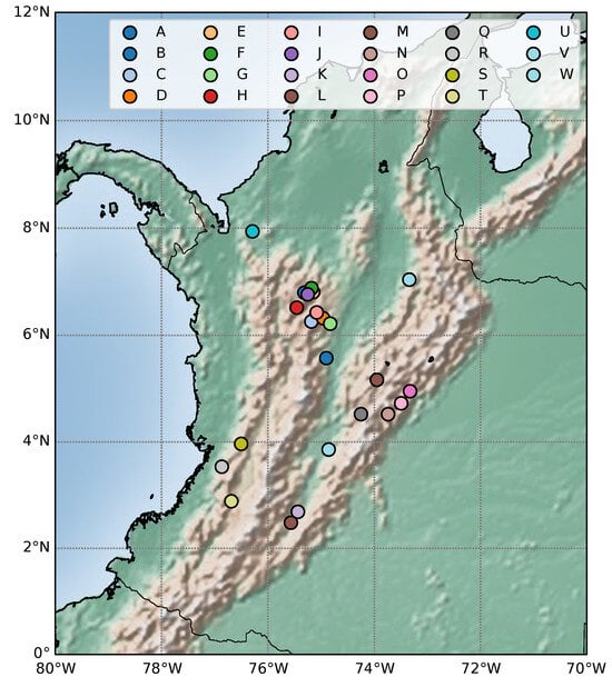
Figure 1.
Reservoir locations in Colombia.
Figure 2 depicts the reservoir-wise data distribution. Firstly, note the wide span of streamflow contributions among reservoirs due to differing power generation capacities. Secondly, most reservoirs hold a non-Gaussian distribution, including platykurtic (such as reservoir C), negatively skewed (reservoir A), positively skewed (reservoir B), long-tailed (reservoir F), and bimodal (reservoir O). The factors leading to the above varying distributions include the atypical rainy days, prolonged dry seasons prevalent in Colombian weather conditions, and operational decisions for enforcing water conservation or maximizing the generation. Further, reservoir Q, which consistently reported zero streamflow, allows for assessing the forecasting performance in trivial cases. For validation purposes, the last two years of data assess the SVGP performance as the testing subset, whereas the first ten years become the training subset with samples.
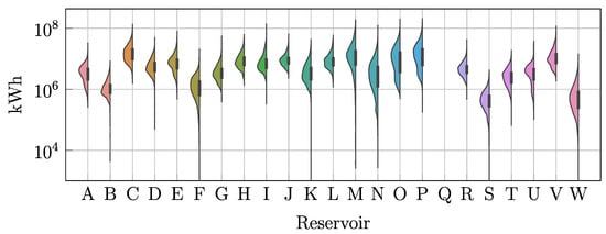
Figure 2.
Time-series Violin plot depicting the streamflow contribution for each reservoir within the dataset.
3.2. Hyperparameter Tuning and Model Interpretability
Given the Colombian streamflow dataset, the hydrological forecasting task corresponds to predicting the reservoir contributions at instant based on the contributions at day n. H stands for the forecasting horizon, including short (up to a week ahead ) and medium-term (up to one month ahead ). To this end, the SVGP demands a fixed number of inducing points M and order size T. Figure 3 presents the grid search results for tuning M and T by minimizing the MSLL and MSE in a ten-fold cross-validation on the training subset at the fixed one-day-ahead forecasting horizon (). Results evidence that the median MSLL and MSE generally decrease when increasing the number of inducing points, up to , after which the error increases, and increase for large values of T. The above is because a few inducing points are more sensitive to initialization and fail to capture the intrinsic phenomenon distribution, thereby underfitting the regression task. On the contrary, too many inducing points and a high order monotonically increase both metrics, indicating a model overfitting. Consequently, the hyperparameter tuning designates inducing points and as the most accurate and consistent within the grid search.
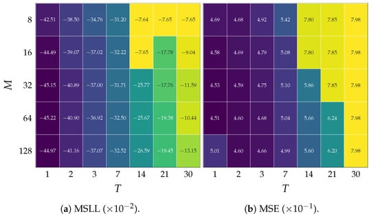
Figure 3.
Grid search results for tuning the model order T and the number of inducing points M. Ten-fold average is reported for MSLL and MSE metrics. The yellow to blue transition indicates a change from worse to better hyperparameters.
Using the tuned number of inducing points M and model order T, Figure 4 presents the trained reservoir-wise output scales and the estimated noise variance for different horizons (H). Overall, the longer the horizon, the smaller the output scale for all reservoirs. The above suggests a reduction in correlation for long horizons, making the SVGP approximate the prior distribution with a time-uncorrelated function. Nonetheless, for reservoirs P and V, an output scale increment at long horizons follows the initial reduction, implying the existence of relevant periodicity components within such time series. Lastly, reservoir Q consistently renders low scale values along horizons to enforce the expected zero streamflow.
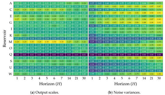
Figure 4.
Trained model Output scales and noise variance parameters for each forecasting horizon and input reservoir. Yellow and blue colors denote large and small parameters values, respectively.
Regarding the noise variance, the heightened unpredictability in the output data at long horizons yields an increment in , which also supports the positive definiteness of the covariance matrix in Equation (4). For such horizons, the model uncertainty mainly depends on the noise variance rather than the output scale. Therefore, the SVGP model exploits the data correlations at short horizons, yielding a low uncertainty while understanding the lack of information for long-horizon forecasting as a zero-mean isotropic Gaussian posterior. Notice that the SVGP is capable of inferring null variance for reservoir Q due to zero streamflow.
The lengthscale analysis relies on its capacity to deactivate nonessential features on a kernel machine according to the Automatic Relevance Determination (ARD) criterion [42,43]. Hence, a small lengthscale value implies a high relevance for predicting the future streamflow of a reservoir from the past of another [44]. Figure 5 depicts the trained lengthscales in Equation (17) from each input feature (columns) to each output task (rows) for prediction horizons of one day (left), two weeks (center), and one month (right). At first glance, reservoir Q exhibits notably small lengthscales, for predicting other reservoirs (Q-th column) and high lengthscales as the target reservoir (Q-th row), misinterpreted as highly relevant according to ARD. As the target reservoir, the zero streamflow during the observation period tunes high lengthscales values due to no relevant features being found. Hence, the SVGP turns off the corresponding rows in (in Equation (4)) and the influence of every reservoir on the posterior mean for the reservoir Q despite its lengthscale. As the predicting reservoir, Q holds N zero terms within the vector in Equation (4), yielding a zero contribution to build the mean posterior of every other reservoir. In either case, the SVGP identifies the influence lack of the reservoir Q and fixes the corresponding lengthscales (rows and columns) to the default value of .
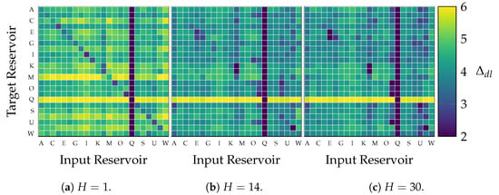
Figure 5.
Trained lengthscales from input feature (columns) to each output task (rows) for three prediction horizons.
The shortest horizon (one day ahead prediction, ) distributes the smallest lengthscale values over the main diagonal contrary to the high off-diagonal values. This result proves the relevance of short-term memory components within each streamflow. At a longer horizon of fourteen days (), the lengthscales over the main diagonal become higher, losing relevance, and several off-diagonal become lower, gaining relevance, than at a one-day horizon. Such a change implies that a reservoir provides less information to predict itself at longer horizons, leading the model to look for knowledge in other reservoirs. The longest horizon () illustrates even less relevant lengthscales, indicating that the SVGP restrains the number of relevant features. Thus, the lengthscale variations across different prediction horizons reveal the dynamic interplay between reservoirs and highlight the Gaussian Process’s ability to select relevant features adaptively.
For visual interpretation of SVGP inner workings, Figure 6 maps in 2D the reservoir data along with the optimized inducing points using the t-distributed Stochastic Neighbor Embedding (t-SNE) technique for each target reservoir. The input-space similarity measure demanded by t-SNE was tailored to the kernel in Equation (17) with the tuned lengthscales for each task, guaranteeing the mapping of the same latent space designed by the SVGP. The filled contours outline the density distribution of training data, whereas the color scatter locates the optimized inducing points. We strategically labeled three inducing points for analyzing the SVGP behavior. Since the forecasting tasks share the inducing points, not the kernel parameters, each target reservoir holds a different t-SNE mapping.
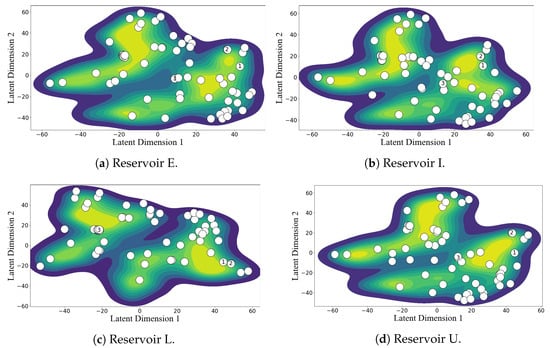
Figure 6.
t-SNE-based two-dimensional mapping of the SVGP latent space and inducing points’ locations for four target reservoirs. We numbered three inducing points for analyzing the model behavior.
The 2D plots exhibit multi-modal distributions for all tasks, indicating clustered information and varying dynamics within a reservoir. Hence, the SVGP trades off the location of the inducing points between the within-task centroids and the among-task relationships. For instance, the locations of points 1 and 2 inducing points emerge near a mode of the four distribution plots, representing global information shared by most tasks. The locations of point 3 also pose a remarkable insight. Simultaneously, the inducing point 3 appears far from any cluster of reservoir E while near a mode of reservoirs L and U, adding information that improves the performance of a few related tasks. Therefore, the shared inducing points allow for the capturing of the task-wise, group-wise, and global information about the streamflow dynamics.
3.3. Performance Analysis
In the case of LSTM, we set up a single multi-output model to forecast all reservoirs simultaneously. The LSTM holds the number of hidden units as a hyperparameter, which we tuned in a grid search strategy, yielding an optimum of one unit.
For performance analysis, the proposed SVGP-based forecasting is contrasted against the straightforward Linear AutoRegressive model (LAR) and the nonlinear Long-Short-Term Memory network (LSTM) [19,45,46,47,48]. Particularly for LAR, we trained a single output model for each task. Further, the frequentist perspective treats the model weights as random estimators following a Gaussian distribution. Such a treatment turns the LAR into a probabilistic model, allowing it to generate confidence intervals for its predictions. In the case of LSTM, we set up a single multi-output model to forecast all reservoirs simultaneously. To tune the number of hidden units of the LSTM, we run a grid search, yielding an optimum of one unit. As a deterministic model, LSTM lacks a predictive distribution and cannot be assessed with the probabilistic performance metrics MSLL and CRPS.
Figure 7 illustrates the testing time series of streamflow contributions and their corresponding one-day ahead predictions generated by the contrasted models for three reservoirs strategically chosen to show different forecasting complexities. The red dots correspond to test data and the green lines denote the LSTM predictions. The yellow and blue lines and regions represent the mean and 95% confidence intervals for the LAR and SVGP predictive distribution, respectively.
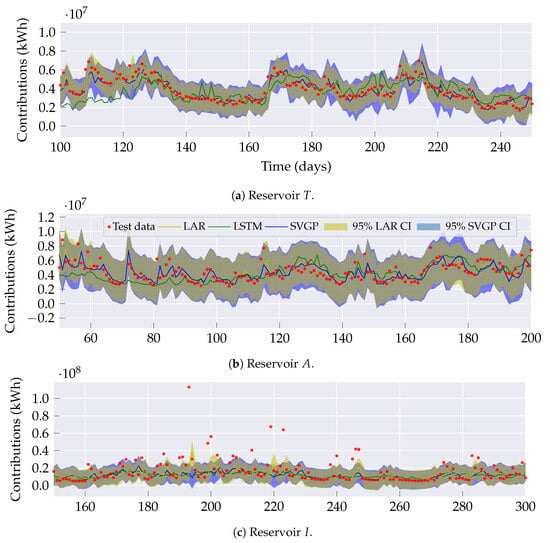
Figure 7.
Test data for reservoirs T (low complexity), A (medium complexity), and I (high complexity) in a one day ahead model’s prediction (). Yellow and blue shaded areas represent the 95% centered confidence interval for the LAR and SVGP predictions, respectively.
Reservoir T in Figure 7a presents the challenge of changing dynamics within the time series, from a steady low variance to a rapidly evolving streamflow. For such a reservoir, SVGP outperforms by better adapting the forecasted dynamics. Reservoir A in Figure 7b portrays a scenario with reduced smoothness with a few abruptly changing segments. Even for those segments, the proposed model tracks the actual curve more closely than LAR and LSTM. Further, the SVGP effectively explains the existence of sudden shifts through its intrinsic confidence intervals. In contrast, reservoir I in Figure 7c exhibits a heavily varying streamflow. Despite the forecasting for the three models diverging from the actual peak values within the time series, the predictive distribution provided by the LAR and SVGP interprets them as outliers. In general, the SVGP is the most adaptative and suitable model to exploit the changing within- and between-reservoir time series, explaining their stochastic nature through the inherent predictive distribution.
Figure 8 and Figure 9 display the overall MSE and MSLL scores achieved by the baseline approaches of LAR and LSTM and the proposed SVGP-based streamflow forecasting over a testing period of two years. Each row represents one target reservoir, whereas the columns indicate the forecasting horizon. The lower plot indicates the grand-average metric along the horizon.
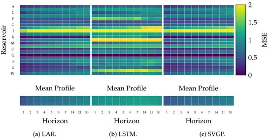
Figure 8.
Achieved MSE for LAR, LSTM, and SVGP forecasting models at each horizon and reservoir.
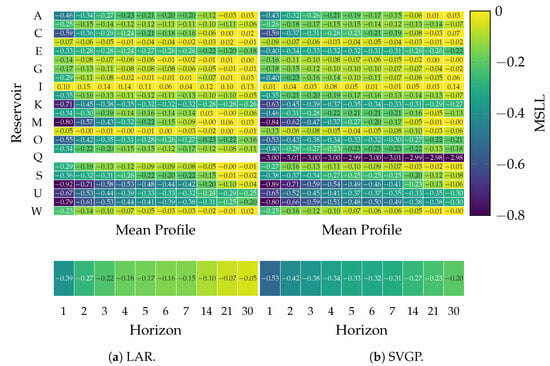
Figure 9.
Achieved MSLL for LAR and SVGP forecasting models at each horizon and reservoir.
As expected, the longer the horizon, the larger the error for all approaches, implying more challenging future forecasting. However, the prediction difficulty varies among reservoirs, with D, H, I, and N as the most demanding, suggesting a lack of information from external factors. In contrast, reservoirs M, T, and V exhibit a less complex streamflow dynamic due to a lower MSLL and MSE. A remarkable observation pertains to reservoir Q, for which the LAR model yields a null MSLL, and the proposed SVGP model achieves the lowest log-likelihood due to a constant zero streamflow. Hence, between the two probabilistic models, the frequentist LAR and the Bayesian SVGP, the latter better represents the steady behavior of reservoir Q.
From one to seven day horizons, the proposed SVGP outperforms MSE in contrast to LAR and LSTM in reservoirs A, C, E, F, and K. Hence, the SVGP effectively captures short-term dependencies in the data. Particularly on reservoir E, the SVGP considerably reduces the error of LSTM, indicating a benefit in capturing short-term dynamics compared to a nonlinear model. As the prediction horizon extends from 14 to 30 days, the SVGP performance remains competitive since its MSE increases slower than LAR and LSTM along the horizon, especially in reservoirs like L, T, and V. Such a fact can also be seen in the grand average MSLL and MSE, where SVGP error remains considerably slower than the baseline models. Concludingly, the Gaussian Process excels in all tested horizons mainly due to the capabilities of nonlinear mapping the data into an infinitely high-dimensional feature space and task-wise adaptation to varying dynamics.
Finally, Table 1 summarizes the MSE, MSLL, and CRPS metrics for the three models (LAR, LSTM, and SVGP), averaged over outputs for each considered horizon. Bold and asterisk indicate that SVGP metrics significantly improve LAR and LSTM in a paired t-test with a 1% p-value. The SVGP model generally outperforms all models except for LAR at horizon H = 1. Such a result indicates a high linear dependence between previous and current time instants. As the horizon increases, the linear dependencies diminish, and the SVGP model unravels the input–output relationships in a high-dimensional feature space via kernel functions. Finally, the grand average over all horizons shows that the SVGP significantly enhances the contrasted models, with the additional advantage of providing a predictive distribution to evaluate forecasting confidence.

Table 1.
Performance metrics for LAR, LSTM, and SVGP on the considered horizons H. Bold and asterisk denote a p-value in a one-tailed paired t-test for LAR vs. SVGP and LSTM vs. SVGP.
4. Concluding Remarks
This work develops a scalable and interpretable streamflow-forecasting methodology based on Sparse Variational Gaussian Processes (SVGPs). Compared to the conventional GPs, the proposed methodology diminishes the computational complexity from cubic to linear regarding the number of samples, becoming more scalable to forecasting tasks on large datasets. In this sense, the proposed SVGP focuses on predicting 23 of Colombia’s reservoir streamflow contributions, geographically distributed nationwide. Due to the widespread locations, time-series dynamics and data distribution vary among reservoirs.
Regarding the hyperparameters, the optimal number of inducing points performs as an inherent regularization by encoding the most information from the data while avoiding overfitting. Such an optimal hyperparameter allows interpretation of the Gaussian Process model in terms of the inducing points and the kernel parameters. On the one hand, the t-SNE-based distribution plots reveal that the proposed model strategically places the shared inducing points to capture task-wise, group-specific, and global dynamics despite the complex, multi-modal nature of reservoir data, trading off between capturing the reservoir-wise unique characteristics and the between-reservoir dependencies, thereby improving the overall performance in streamflow forecasting. On the other hand, the trained lengthscales prove that the GP model successfully adjusts its focus to prediction horizon changes between short-term memory components (using the past data of the reservoir itself) and long-term relationships (exploiting interactions between different reservoirs). This adaptability makes the Gaussian Process model robust and versatile for multiple-output forecasting tasks with varying time features.
The performance analysis evidences the advantage of the SVGP-based model over the baseline Linear Autoregressive (LAR) model and Long Short-Term Memory network (LSTM) for streamflow prediction in three main aspects. The performance analysis evidences the advantage of the proposed SVGP model over the baseline Linear Autoregressive (LAR) model and nonlinear Long Short-Term Memory network (LSTM) for streamflow prediction in three main aspects. Firstly, the proposed approach suitably adapts to changing dynamics within and between reservoirs, even on rapidly changing time series or abrupt shifts. Secondly, the Bayesian scheme makes the proposed methodology predict the streamflow as the mean of an intrinsic posterior distribution and provides informative confidence intervals through its posterior variance. Thirdly, the SVGP better copes with the enhanced forecasting complexity for long horizons than baseline approaches, as proved by the slower error growth. Overall, the proposed SVGP-based methodology efficiently captures and adapts to the complex and stochastic nature of the streamflow contribution time series, enhancing the forecasting task on multiple horizons.
For pursuing the research on SVGP-based hydrological forecasting, three directions are advised: The first research direction aims to integrate SVGP-based streamflow forecasting into the scheduling algorithms of thermoelectric power plants. Such an integrated approach will support a resilient and efficient energy system by optimizing the operation of hydroelectric and thermoelectric resources. Another future work is related to the fact that the reservoirs become operational at different dates. Then, the SVGP-based forecasting must focus on maintaining a suitable performance on missing data scenarios. One last research in the artificial intelligence field explores how to provide non-Gaussian likelihoods following a better fitting of the constraints of the output distribution, e.g., non-negative streamflow data. Such an approach can be extended to a chained GP framework, allowing each likelihood parameter to follow a GP and enhancing the model flexibility to handle the complex dynamic of hydrological time series.
Author Contributions
Conceptualization, J.D.P.-C. and D.A.C.-P.; methodology, J.D.P.-C.; validation, D.A.C.-P.; formal analysis, A.M.Á.-M.; resources, Á.A.O.-G.; data curation, J.G.-G.; writing—original draft preparation, J.D.P.-C.; writing—review and editing, D.A.C.-P. and Á.A.O.-G.; supervision, Á.A.O.-G. All authors have read and agreed to the published version of the manuscript.
Funding
Under grants provided by research projects 1110-852-69982 (funded by MINCIENCIAS), E6-24-3 (funded by UTP), and the graduate program of Maestría en Ingeniería Eléctrica (UTP).
Data Availability Statement
The data supporting the findings of this study are available on request from the corresponding author, Julián David Pastrana-Cortés. The data are not publicly available due to confidential agreements.
Conflicts of Interest
The authors declare no conflicts of interest.
References
- Tofiq, Y.M.; Latif, S.D.; Ahmed, A.N.; Kumar, P.; El-Shafie, A. Optimized Model Inputs Selections for Enhancing River Streamflow Forecasting Accuracy Using Different Artificial Intelligence Techniques. Water Resour. Manag. 2022, 36, 5999–6016. [Google Scholar] [CrossRef]
- Hojjati-Najafabadi, A.; Mansoorianfar, M.; Liang, T.; Shahin, K.; Karimi-Maleh, H. A review on magnetic sensors for monitoring of hazardous pollutants in water resources. Sci. Total. Environ. 2022, 824, 153844. [Google Scholar] [CrossRef] [PubMed]
- Mensah, J.K.; Ofosu, E.A.; Yidana, S.M.; Akpoti, K.; Kabo-bah, A.T. Integrated modeling of hydrological processes and groundwater recharge based on land use land cover, and climate changes: A systematic review. Environ. Adv. 2022, 8, 100224. [Google Scholar] [CrossRef]
- Sulamo, M.A.; Kassa, A.K.; Roba, N.T. Evaluation of the impacts of land use/cover changes on water balance of Bilate watershed, Rift valley basin, Ethiopia. Water Pract. Technol. 2021, 16, 1108–1127. [Google Scholar] [CrossRef]
- Huang, J.; Cang, J.; Zhou, Z.; Gholinia, F. Evaluation effect climate parameters change on hydropower production and energy demand by RCPs scenarios and the Developed Pathfinder (DPA) algorithm. Energy Rep. 2021, 7, 5455–5466. [Google Scholar] [CrossRef]
- Beça, P.; Rodrigues, A.C.; Nunes, J.P.; Diogo, P.; Mujtaba, B. Optimizing Reservoir Water Management in a Changing Climate. Water Resour. Manag. 2023, 37, 3423–3437. [Google Scholar] [CrossRef]
- Departamento Nacional de Planeación. Bases del Plan Nacional de Inversiones 2022–2026; Documento en Línea; Departamento Nacional de Planeación: Bogota, Columbia, 2023. [Google Scholar]
- Unidad de Planeación Minero Energética (UPME). Mapa Energético de Colombia; Documento en líNea; UPME: Bogota, Columbia, 2019. [Google Scholar]
- Coronado-Hernández, Ó.E.; Merlano-Sabalza, E.; Díaz-Vergara, Z.; Coronado-Hernández, J.R. Selection of Hydrological Probability Distributions for Extreme Rainfall Events in the Regions of Colombia. Water 2020, 12, 1397. [Google Scholar] [CrossRef]
- Yaseen, Z.M.; Allawi, M.F.; Yousif, A.A.; Jaafar, O.; Hamzah, F.M.; El-Shafie, A. Non-tuned machine learning approach for hydrological time series forecasting. Neural Comput. Appl. 2018, 30, 1479–1491. [Google Scholar] [CrossRef]
- H. Kashani, M.; Ghorbani, M.A.; Dinpashoh, Y.; Shahmorad, S. Integration of Volterra model with artificial neural networks for rainfall-runoff simulation in forested catchment of northern Iran. J. Hydrol. 2016, 540, 340–354. [Google Scholar] [CrossRef]
- Li, P.; Zha, Y.; Shi, L.; Tso, C.H.M.; Zhang, Y.; Zeng, W. Comparison of the use of a physical-based model with data assimilation and machine learning methods for simulating soil water dynamics. J. Hydrol. 2020, 584, 124692. [Google Scholar] [CrossRef]
- Lo Iacono, G.; Armstrong, B.; Fleming, L.E.; Elson, R.; Kovats, S.; Vardoulakis, S.; Nichols, G.L. Challenges in developing methods for quantifying the effects of weather and climate on water-associated diseases: A systematic review. PloS Neglected Trop. Dis. 2017, 11, e0005659. [Google Scholar] [CrossRef] [PubMed]
- Cheng, M.; Fang, F.; Kinouchi, T.; Navon, I.; Pain, C. Long lead-time daily and monthly streamflow forecasting using machine learning methods. J. Hydrol. 2020, 590, 125376. [Google Scholar] [CrossRef]
- Kim, T.; Yang, T.; Gao, S.; Zhang, L.; Ding, Z.; Wen, X.; Gourley, J.J.; Hong, Y. Can artificial intelligence and data-driven machine learning models match or even replace process-driven hydrologic models for streamflow simulation?: A case study of four watersheds with different hydro-climatic regions across the CONUS. J. Hydrol. 2021, 598, 126423. [Google Scholar] [CrossRef]
- Baur, L.; Ditschuneit, K.; Schambach, M.; Kaymakci, C.; Wollmann, T.; Sauer, A. Explainability and interpretability in electric load forecasting using machine learning techniques—A review. Energy AI 2024, 16, 100358. [Google Scholar] [CrossRef]
- Sit, M.; Demiray, B.Z.; Xiang, Z.; Ewing, G.J.; Sermet, Y.; Demir, I. A comprehensive review of deep learning applications in hydrology and water resources. Water Sci. Technol. 2020, 82, 2635–2670. [Google Scholar] [CrossRef] [PubMed]
- Guo, J.; Liu, Y.; Zou, Q.; Ye, L.; Zhu, S.; Zhang, H. Study on optimization and combination strategy of multiple daily runoff prediction models coupled with physical mechanism and LSTM. J. Hydrol. 2023, 624, 129969. [Google Scholar] [CrossRef]
- Sahoo, B.B.; Jha, R.; Singh, A.; Kumar, D. Long short-term memory (LSTM) recurrent neural network for low-flow hydrological time series forecasting. Acta Geophys. 2019, 67, 1471–1481. [Google Scholar] [CrossRef]
- Tebong, N.K.; Simo, T.; Takougang, A.N. Two-level deep learning ensemble model for forecasting hydroelectricity production. Energy Rep. 2023, 10, 2793–2803. [Google Scholar] [CrossRef]
- Moon, J.; Park, S.; Rho, S.; Hwang, E. Interpretable short-term electrical load forecasting scheme using cubist. Comput. Intell. Neurosci. 2022, 2022, 6892995. [Google Scholar] [CrossRef]
- Gal, Y.; Ghahramani, Z. Dropout as a Bayesian approximation: Representing model uncertainty in deep learning. In Proceedings of the International Conference on Machine Learning, New York, NY, USA, 20–22 June 2016; pp. 1050–1059. [Google Scholar]
- Lakshminarayanan, B.; Pritzel, A.; Blundell, C. Simple and Scalable Predictive Uncertainty Estimation using Deep Ensembles. arXiv 2017, arXiv:1612.01474. [Google Scholar]
- Wang, B.; Li, T.; Yan, Z.; Zhang, G.; Lu, J. DeepPIPE: A distribution-free uncertainty quantification approach for time series forecasting. Neurocomputing 2020, 397, 11–19. [Google Scholar] [CrossRef]
- Quilty, J.; Adamowski, J. A stochastic wavelet-based data-driven framework for forecasting uncertain multiscale hydrological and water resources processes. Environ. Model. Softw. 2020, 130, 104718. [Google Scholar] [CrossRef]
- Cárdenas-Peña, D.; Collazos-Huertas, D.; Álvarez Meza, A.; Castellanos-Dominguez, G. Supervised kernel approach for automated learning using General Stochastic Networks. Eng. Appl. Artif. Intell. 2018, 68, 10–17. [Google Scholar] [CrossRef]
- Wen, H.; Ma, J.; Gu, J.; Yuan, L.; Jin, Z. Sparse Variational Gaussian Process Based Day-Ahead Probabilistic Wind Power Forecasting. IEEE Trans. Sustain. Energy 2022, 13, 957–970. [Google Scholar] [CrossRef]
- Eressa, M.R.; Badis, H.; George, L.; Grosso, D. Sparse Variational Gaussian Process with Dynamic Kernel for Electricity Demand Forecasting. In Proceedings of the 2022 IEEE 7th International Energy Conference (ENERGYCON), Riga, Latvia, 9–12 May 2022; pp. 1–6. [Google Scholar] [CrossRef]
- Niu, W.J.; Feng, Z.K. Evaluating the performances of several artificial intelligence methods in forecasting daily streamflow time series for sustainable water resources management. Sustain. Cities Soc. 2021, 64, 102562. [Google Scholar] [CrossRef]
- Sun, A.Y.; Wang, D.; Xu, X. Monthly streamflow forecasting using Gaussian Process Regression. J. Hydrol. 2014, 511, 72–81. [Google Scholar] [CrossRef]
- Sun, N.; Zhang, S.; Peng, T.; Zhang, N.; Zhou, J.; Zhang, H. Multi-Variables-Driven Model Based on Random Forest and Gaussian Process Regression for Monthly Streamflow Forecasting. Water 2022, 14, 1828. [Google Scholar] [CrossRef]
- Park, H.J.; Kim, Y.; Kim, H.Y. Stock market forecasting using a multi-task approach integrating long short-term memory and the random forest framework. Appl. Soft Comput. 2022, 114, 108106. [Google Scholar] [CrossRef]
- Liu, C.L.; Tseng, C.J.; Huang, T.H.; Yang, J.S.; Huang, K.B. A multi-task learning model for building electrical load prediction. Energy Build. 2023, 278, 112601. [Google Scholar] [CrossRef]
- Dong, L.; Li, Y.; Xiu, X.; Li, Z.; Zhang, W.; Chen, D. An integrated ultra short term power forecasting method for regional wind–pv–hydro. Energy Reports 2023, 9, 1531–1540. [Google Scholar] [CrossRef]
- Álvarez, M.A.; Rosasco, L.; Lawrence, N.D. Kernels for Vector-Valued Functions: A Review; Now Foundations and Trends; ACM: New York, NY, USA, 2012. [Google Scholar]
- Bruinsma, W.; Perim, E.; Tebbutt, W.; Hosking, S.; Solin, A.; Turner, R. Scalable Exact Inference in Multi-Output Gaussian Processes. In Proceedings of the 37th International Conference on Machine Learning, Virtual, 13–18 July 2020; Daumé, H., Singh, A., Eds.; ACM: New York, NY, USA, 2020; Volume 119, pp. 1190–1201. [Google Scholar]
- Liu, H.; Cai, J.; Ong, Y.S. Remarks on multi-output Gaussian process regression. Knowl.-Based Syst. 2018, 144, 102–121. [Google Scholar] [CrossRef]
- Ditthakit, P.; Pinthong, S.; Salaeh, N.; Weekaew, J.; Thanh Tran, T.; Bao Pham, Q. Comparative study of machine learning methods and GR2M model for monthly runoff prediction. Ain Shams Eng. J. 2023, 14, 101941. [Google Scholar] [CrossRef]
- Hensman, J.; Fusi, N.; Lawrence, N.D. Gaussian Processes for Big Data. arXiv 2013, arXiv:1309.6835. [Google Scholar] [CrossRef]
- Hensman, J.; Matthews, A.; Ghahramani, Z. Scalable Variational Gaussian Process Classification. In Proceedings of the 18th International Conference on Artificial Intelligence and Statistics, San Diego, CA, USA, 9–12 May 2015; Lebanon, G., Vishwanathan, S.V.N., Eds.; ACM: New York, NY, USA, 2015; Volume 38, pp. 351–360. [Google Scholar]
- Rasmussen, C.E.; Williams, C.K.I. Gaussian Processes for Machine Learning; Adaptive Computation and Machine Learning; MIT Press: Cambridge, MA, USA, 2006; pp. I–XVIII, 1–248. [Google Scholar]
- Liu, K.; Li, Y.; Hu, X.; Lucu, M.; Widanage, W.D. Gaussian Process Regression With Automatic Relevance Determination Kernel for Calendar Aging Prediction of Lithium-Ion Batteries. IEEE Trans. Ind. Inform. 2020, 16, 3767–3777. [Google Scholar] [CrossRef]
- Damianou, A.; Lawrence, N.D. Deep Gaussian Processes. In Proceedings of the 16th International Conference on Artificial Intelligence and Statistics, Scottsdale, AZ, USA, 29 April–1 May 2013; Carvalho, C.M., Ravikumar, P., Eds.; ACM: New York, NY, USA, 2013; Volume 31, pp. 207–215. [Google Scholar]
- Cárdenas-Peña, D.; Collazos-Huertas, D.; Castellanos-Dominguez, G. Enhanced Data Representation by Kernel Metric Learning for Dementia Diagnosis. Front. Neurosci. 2017, 11, 413. [Google Scholar] [CrossRef] [PubMed]
- Rahimzad, M.; Moghaddam Nia, A.; Zolfonoon, H.; Soltani, J.; Danandeh Mehr, A.; Kwon, H.H. Performance Comparison of an LSTM-based Deep Learning Model versus Conventional Machine Learning Algorithms for Streamflow Forecasting. Water Resour. Manag. 2021, 35, 4167–4187. [Google Scholar] [CrossRef]
- Kilinc, H.C.; Haznedar, B. A Hybrid Model for Streamflow Forecasting in the Basin of Euphrates. Water 2022, 14, 80. [Google Scholar] [CrossRef]
- Hu, Y.; Yan, L.; Hang, T.; Feng, J. Stream-Flow Forecasting of Small Rivers Based on LSTM. arXiv 2020, arXiv:2001.05681. [Google Scholar]
- Li, J.; Yuan, X. Daily Streamflow Forecasts Based on Cascade Long Short-Term Memory (LSTM) Model over the Yangtze River Basin. Water 2023, 15, 1019. [Google Scholar] [CrossRef]
Disclaimer/Publisher’s Note: The statements, opinions and data contained in all publications are solely those of the individual author(s) and contributor(s) and not of MDPI and/or the editor(s). MDPI and/or the editor(s) disclaim responsibility for any injury to people or property resulting from any ideas, methods, instructions or products referred to in the content. |
© 2024 by the authors. Licensee MDPI, Basel, Switzerland. This article is an open access article distributed under the terms and conditions of the Creative Commons Attribution (CC BY) license (https://creativecommons.org/licenses/by/4.0/).