Water Level Prediction and Forecasting Using a Long Short-Term Memory Model for Nam Ngum River Basin in Lao PDR

Abstract

The process of implementing neural networks in a computer system is known as deep learning. In this study, a deep learning model, namely long short-term memory (LSTM), was established to predict and forecast water levels for stations located at the Nam Ngum River Basin in Lao PDR. Water levels are predicted and forecasted based on the rainfall and water level data observed at previous time steps. It is proposed that the optimal sequence length for modeling should be determined based on the threshold of the correlation coefficient obtained from the water level and rainfall time series. The trained LSTM models in this study can be considered fair and adequate for water level prediction, as NSE values from 0.5 to 0.7 were mostly obtained from the model validations in the testing periods. The results showed that the autocorrelation and cross-correlation analysis did help in determining the optimal sequence length in an LSTM model. The performance levels of the LSTM model in forecasting future water levels in the Nam Ngum River Basin varied; the forecasted water level hydrographs for the Pakkayoung station generally corresponded with the observed ones, while the forecasted water level hydrographs for the other stations deviated significantly from the observed hydrographs.

1. Introduction

As our global community faces escalating water challenges driven by climate change, population growth, and pollution, the need for innovative solutions and informed decision making becomes increasingly urgent [1]. The application of machine learning for hydrological modeling has prevailed since its emergence about 40 years ago. More data are available at present, compared to the past, allowing the application of machine learning to blossom in various fields, growing exponentially in the last decade. Water level prediction and forecasting are crucial for water resource management and flood monitoring. Traditionally, various approaches such as using regression between gauges and rainfall–runoff modeling have been used to predict and forecast water levels [2,3,4,5,6].

The results of data-driven modeling such as deep learning simulations in hydrology are greatly dependent on the structure of the models and the composition of the input data used for learning. Therefore, significant research efforts have been devoted to determining the appropriate combinations of input data and model structures for deep learning simulations in hydrology. Kim and Kang [7] analyzed the prediction accuracy of the model obtained from various combinations of input data by considering different numbers of hidden layers of long short-term memory (LSTM), the amount of data used for learning, and the characteristics of the learning data. The optimized sets of input data were then used in an appropriate LSTM model structure to improve the prediction of runoff.

Lee and Hwang [8] proposed an artificial neural network (ANN)-based water level prediction model using the water level and rainfall observed at the nearby monitoring stations as the inputs to predict the water level of small- and medium-sized rivers with limited observed data. Again, several scenarios were adopted in the simulations in order to locate the best configuration of datasets to construct an appropriate water level prediction model for acquiring the most promising results. Hidayat et al. [9] attempted to estimate the water level of tidal streams affected by tidal waves using an ANN model; the authors also constructed a real-time water level prediction system using the observed upstream water level and discharge and the downstream tidal data as model learning data for runoff/outflow estimation. The best configurations of input data were identified by comparing the outputs from each configuration to the actual values with minimal errors.

Establishing a deep learning model for applications in hydrology requires a process of verifying the applicability of the model for practical use. Kim et al. [10] developed an LSTM model to predict the water level using the historical water level and rainfall data at the same point, and the applicability of the model was proven by evaluating the prediction accuracy of the model according to the lead time. Lee et al. [11] simulated the outflow at the lower Mekong River using both physical models and data-driven models, and the performance levels of these two models were evaluated. The authors concluded that the accuracy of the data-driven model was better, demonstrating that the data-driven model in fact outperformed the conventional physical model. Jung et al. [12] developed a water level prediction model for the Jamsu Bridge of the Han River through an LSTM model by utilizing the outflow discharged from the Paldang Dam, the tide level observed at the Ganghwa Bridge, and the historical water level time series data at Jamsu Bridge as learning data. In addition, the performance of the model was also evaluated according to the lead time. It was found that the optimized lead time for the constructed model was 1 h, and the prediction performance of the model decreased as the lead time increased.

Le et al. [13] constructed an LSTM model for the prediction of flood volume at the Hoa Binh catchment in the Da River Basin, Vietnam, using the historical observed daily discharge and rainfall levels as the input data. The performance of the model was evaluated according to various aspects such as the lead time and configurations as well as the characteristics of the input datasets. Hu et al. [14] computed a runoff estimation model by analyzing the relationship between the historical rainfall and runoff time series data using ANN and LSTM models. Twelve flood events were selected as learning materials, and it was found that the prediction accuracy decreased with an increasing lead time in both models.

Additionally, deep learning algorithms have also been applied for flood prevention and management. For example, Fang et al. [15] prepared a flood vulnerability map using an LSTM model to predict the likelihood of flooding according to the environmental and terrain characteristics of the basin. The terrain characteristics of the basin such as altitude, curvature, and land use were processed and extracted from a widely used Geographic Information System (GIS) software package called ArcGIS (https://www.sciencedirect.com/science/article/pii/S0022169420311951?via%3Dihub: accessed on 7 January 2024). The relationship between the flood occurrences and respective influencing terrain characteristics was analyzed through the LSTM model. Then, the weight of each factor was obtained, and a map indicating the flood vulnerability of the basin was produced.

Many studies have been conducted to assess the feasibility of data-driven modeling in estimating the streamflow or water level in a river by comparing to the results produced from the conventional, process-driven rainfall–runoff models such as the soil moisture accounting (SMA) model. The majority of these studies conclude that data-driven modeling using deep learning algorithms like LSTM outperforms conventional rainfall–runoff models, especially for basins with sufficient high-quality observed datasets. Recently, data-driven modeling has also been extended for application in ungauged basins where observed datasets are either not available or scarce. Even the IT giant Google has been actively involved in this field, recently releasing Flood Hub, an LSTM-based flood forecasting system, to the public. This system is developed for issuing flood warnings/alerts based on the forecasted future 7-day water level estimated from LSTM modeling for particular gauged and ungauged river basins located all over the world.

However, we noticed that many studies have concluded that the data-driven modeling performed better than the conventional rainfall runoff modeling based on the prediction results using historical observed data. In other words, they solely compared and evaluated the simulated results (streamflow or water level) obtained from both data-driven modeling and conventional rainfall runoff modeling for a single storm event or series of storm events that happened in the past. The assessment of data-driven modeling in forecasting streamflow or future water levels remains under-explored. Since there have already been many studies conducted on the performance of data-driven modeling for predicting either streamflow or water level, this study fills a research gap by not only studying the performance of an LSTM model in predicting historical water levels but also for forecasting future water levels. In addition, we propose defining the optimal sequence length for LSTM modeling based on the threshold of correlation coefficients obtained from water level and rainfall time series through autocorrelation and cross-correlation analysis.

2. Materials and Methods

2.1. Study Area

The Nam Ngum River Basin is of vital importance to the Lao PDR, as it plays the role of major food supplier to the country. The Nam Ngum River, the main river in the basin, originates from the north-east of the basin and flows down towards the south for about 420 km where it converges with its main tributary, the Nam Lik River. After joining with the Nam Lik River, the Nam Ngum River will eventually drain to Mekong River at Pak Ngum. The total catchment area for the Nam Ngum River Basin, which is indicated as a red boundary in Figure 1, is about 17,000 km².

The mean annual rainfall of the basin is about 2000 mm, ranging from 1200 mm to 3500 mm across the basin [16]. The wet season usually starts in June and ends in October, followed by a distinct dry season for the rest of the year. It is estimated that the Nam Ngum River Basin contributes an average annual discharge of about 21,000 million cubic meters (mcm) to the Mekong River [16].

The Nam Ngum reservoir, located downstream of the Nam Ngum River, has a surface area of about 370 km² and a storage capacity of 7010 mcm, thus facilitating Nam Ngum 1 (NN1), the largest hydropower station in the river basin. The NN1 station was completed in 1971 and boasts an installed capacity of 155 MW [16].

It has been mentioned by the Mekong River Commission (MRC) that the downstream regions of the Nam Ngum River Basin have been suffering from reoccurring floods, especially during the annual wet season. To this end, myriad studies and projects on flood prevention and mitigation have been initiated in recent years, and hydrological observation sites such as rainfall and water level stations have also been established along the Nam Ngum River to enable the close monitoring of flood occurrences within the river basin.

Relevant hydrological data have been collected from four hydrological stations located within the Nam Ngum River Basin, namely Phiangluang, Thalad, Pakkayoung, and Veunkham. The Phiangluang station is located upstream of the Nam Ngum River, while Thalad, Pakkayoung, and Veunkham stations are located downstream of the Nam Ngum reservoir and river. Figure 1 illustrates the location of the hydrological stations that will be utilized for analysis in this study, and the coordinates of the rainfall and water level stations are identical. The details of these selected hydrological stations are summarized in

Table 1. List of selected hydrological stations and respective locations.

No.	Station	Latitude	Longitude
1	Phiangluang	19°34′06″ N	103°04′17″ E
2	Thalad	18°31′26″ N	102°30′54″ E
3	Pakkayoung	18°25′53″ N	102°32′16″ E
4	Veunkham	18°10′37″ N	102°36′53″ E

.

Table 2. Statistical values of hydrological variables for selected stations in the Nam Ngum River Basin.

	Rainfall (mm)			Water Level (m)
Station	Annual Average	Max.	Average	Max.	Average	Min
Phiangluang	1283	155.8	3.8	8.72	0.79	0.35
Thalad	1515	118.5	4.5	10.95	6.09	0.64
Pakkayoung	1629	111.5	4.8	8.72	3.95	2.28
Veunkham	1651	142.8	4.9	9.10	2.71	0

summarizes the statistical values of the hydrological variables for the selected stations in the Nam Ngum River Basin. It is noteworthy that the highest annual average rainfall of 1651 mm was recorded at the Veunkham station, located downstream of the Nam Ngum River. Conversely, the lowest annual average rainfall of 1283 mm and highest daily rainfall of 155.8 mm were recorded at the Phiangluang station, located the furthest upstream of the Nam Ngum River. A similar pattern has also been observed in the average water level, where the lowest average water level was recorded at the Phiangluang station (located furthest upstream), and the stations located downstream recorded higher water level relatively.

2.2. Data Availability

The daily rainfall and water level data collected from the 4 selected stations located within the Nam Ngum River Basin will be used for training the deep learning model in this study. The data are available from January 2019 to October 2021 for each selected station. The periods with missing data will be dropped and excluded from the training of the model. The amount of missing data for stations Phiangluang, Thalad, and Veunkham is depicted in

Table 3. Availability of hydrological data in respective stations.

Station	Rainfall (RF)	Water Level (WL)	Amount of Available Data (Day)	Missing Data (Day)
Phiangluang	1 January 2019~14 October 2021	1 January 2019~14 October 2021	1017	1
Thalad	1 January 2019~11 October 2021	1 January 2019~11 October 2021	1014	1
Pakkayoung	1 January 2019~11 October 2021	1 January 2019~11 October 2021	1015	-
Veunkham	1 January 2019~10 October 2021	1 January 2019~10 October 2021	1012	2

. The plots of water levels against rainfall time series for each respective station are illustrated in Figure 2.

3. Methodology

3.1. Long Short-Term Memory Network (LSTM)

LSTM is a type of recurrent neural network (RNN), which is a branch of ANN introduced by [17]. LSTM is designed to solve the problem of long-term memory dependence, in which information from the previous point is not sufficiently transmitted as the interval between information points increases in the learning process of the existing recurrent neural network, and it is a technique that solves problems such as the oblique loss of existing recurrent neural networks [18]. Based on the literature reviews presented in previous section, LSTM has been identified as one of the appropriate DL algorithms capable of learning and describing the complex relationships in hydrological phenomena such as the generation of surface runoff and flood volume.

LSTM consists of an input layer, a memory cell, and an output layer. The main feature of LSTM is that it contains a hidden layer called a memory cell. Each memory cell has three gates composed of a forget gate, an input gate, and an output gate for adjusting the state of the cell. Here, the forgetting statement uses a sigmoid function to determine how well to remember the characteristics of each variable in the previous time step. The input statement updates the values (weights) associated with the current time step variables in the previous time step. The output statement uses the output of the previous time step and the variables of the current time step to calculate the output value in the current state [7]. Figure 3 demonstrates the typical architecture structure of an LSTM.

3.2. Structure of Input Data

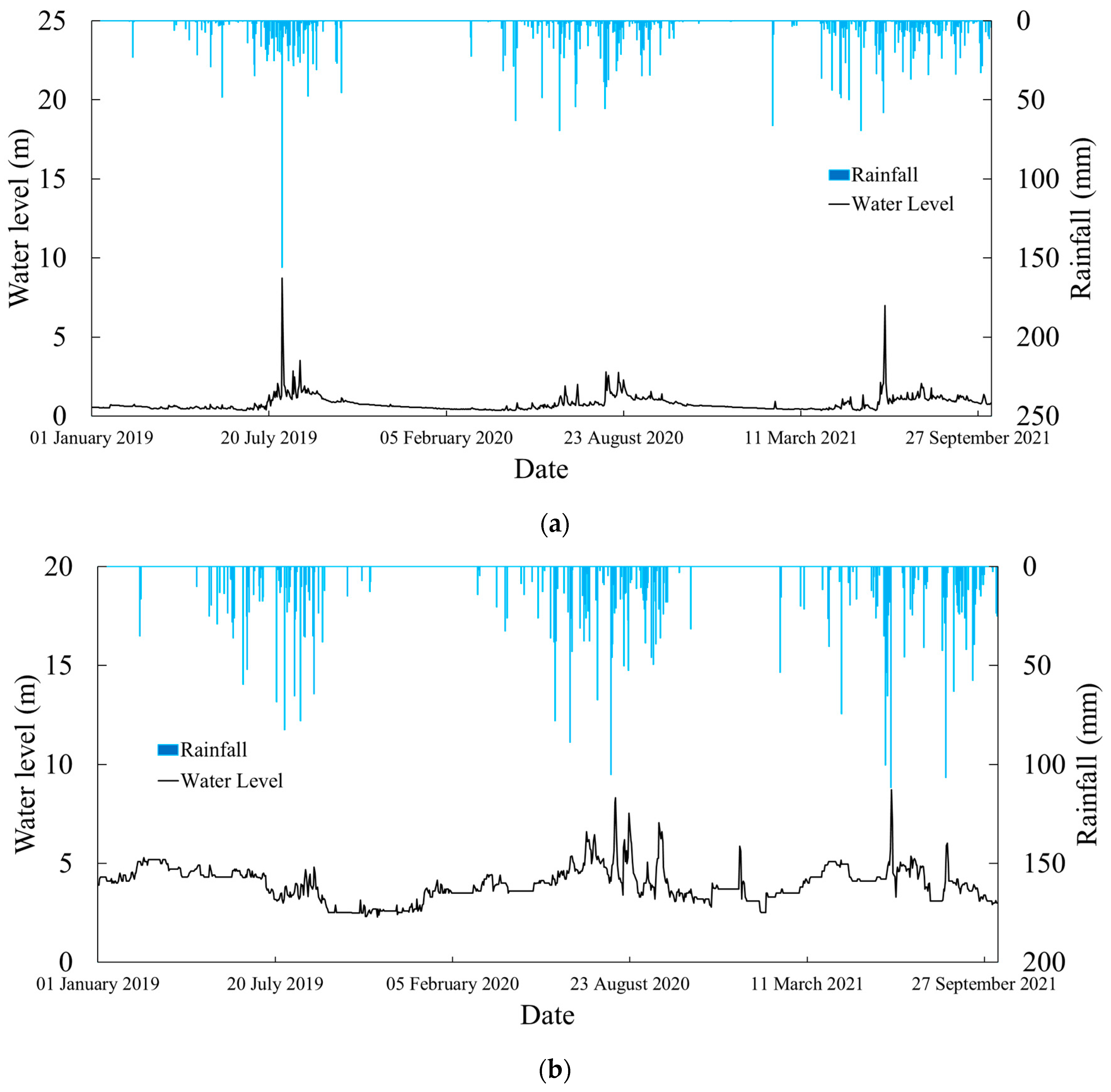
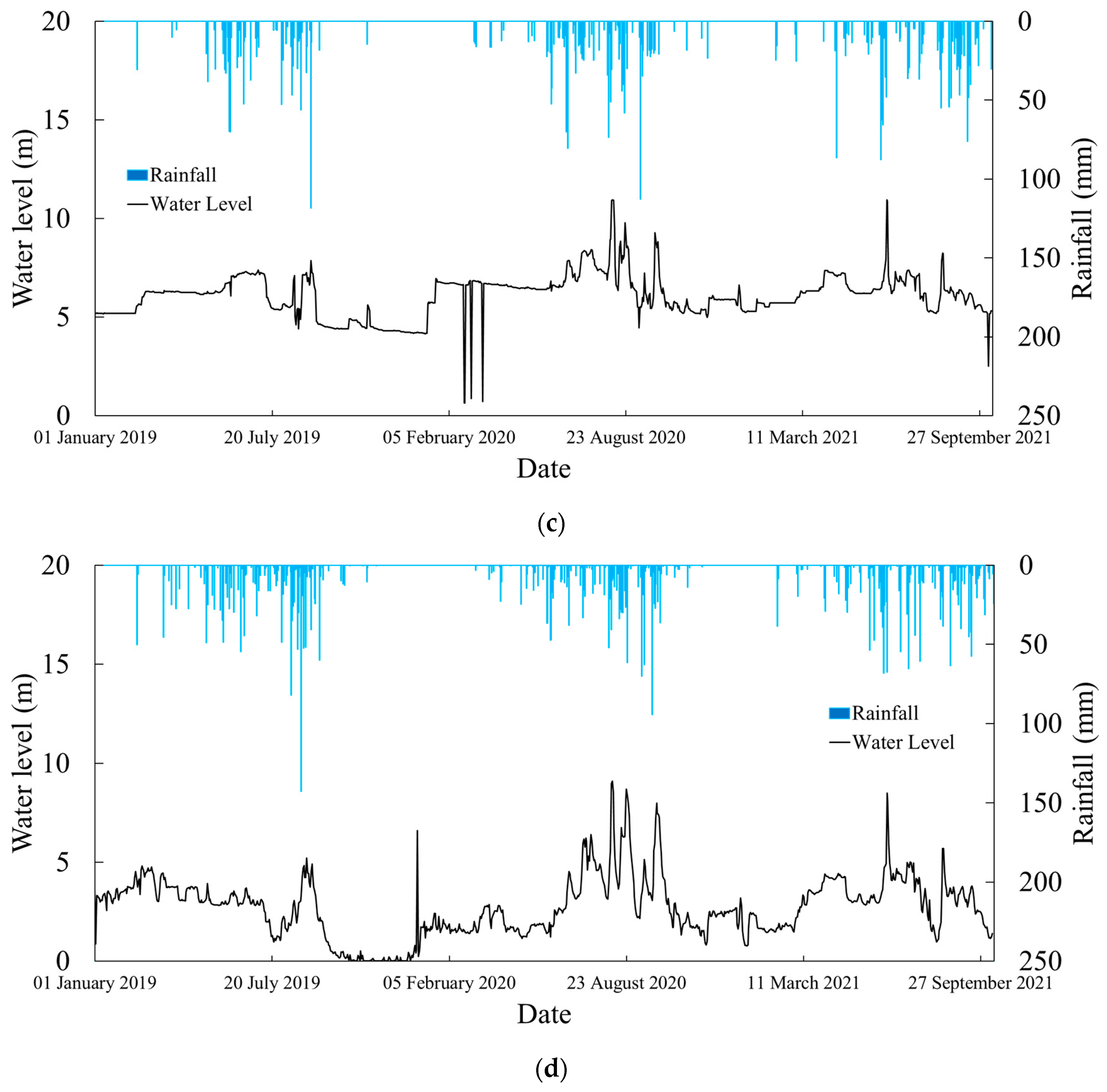
The input data required for water level prediction based on LSTM consist of independent variables and a dependent variable. In this study, the current rainfall (X₁) and water level (X₂) data were entered as the independent variables (X_1,2(t)), while the water level after 1 day was inserted as the dependent variable (Y₁(t + 1)). This type of learning algorithm is known as supervised learning. A conversion code has been written in Python to convert the raw input data into a format which is readable by the supervised learning algorithm in the LSTM model established in this study. In addition, the input data will also be converted into a three-dimensional form (x, y, z), which suits the input form of the LSTM cell. Again, this conversion will also be performed using Python’s reshape code.

In machine learning, sequence length refers to the period of time series data for learning. For example, if the sequence length of data with a time step of 1 day is set to 3, the data at current time X(t), 1 day ago X(t − 1), and 2 days ago X(t − 2) are used as the input variables, and the predicted/forecasted data for the next day Y(t + 1) will be produced as the output/result.

Table 4. The structures of inputs and output applied for LSTM modeling.

Inputs (X)		Output (Y)
Rainfall at current time	Water level at current time	Water level after n days
X1(t)	X2(t)	Y(t + n)

indicates the structures of the model. The setting of the forecast time can be changed by adjusting the lead time. Therefore, the sequence length as well as the lead time applied for modeling and forecasting will be based on the results concluded from the autocorrelation and cross-correlation analysis between the rainfall and water level time series, as explained in Section 3.6.

3.3. Normalization of Input Data

It is common to convert the numerical input data inserted in the model to numbers in a range between 0 and 1. This transformation is known as normalization. If the scale of each variable is different when training the model, it will induce a negative impact on the algorithm’s ability to determine the weight of the variable. Therefore, the data are normalized for the purpose of unifying the scale of each variable so that it reflects the same degree of weight. There are various methods for normalization, such as min–max normalization, Z-score normalization, and standard normalization. Min–max normalization, which uses the MinMax Scaler function of the sklearn package provided by Python 3.10.12, will be applied in this study, and it is described in Equation (1) as follows:

$$x_{norm}=\frac{x-X_{\min }}{X_{\max }-X_{\min }}$$

(1)

where x represents the value to be normalized, X_min and X_max refer to the minimum and maximum values of the variable set containing the value to be normalized, and x_norm describes the normalized value.

3.4. Separation of Data for Training and Testing

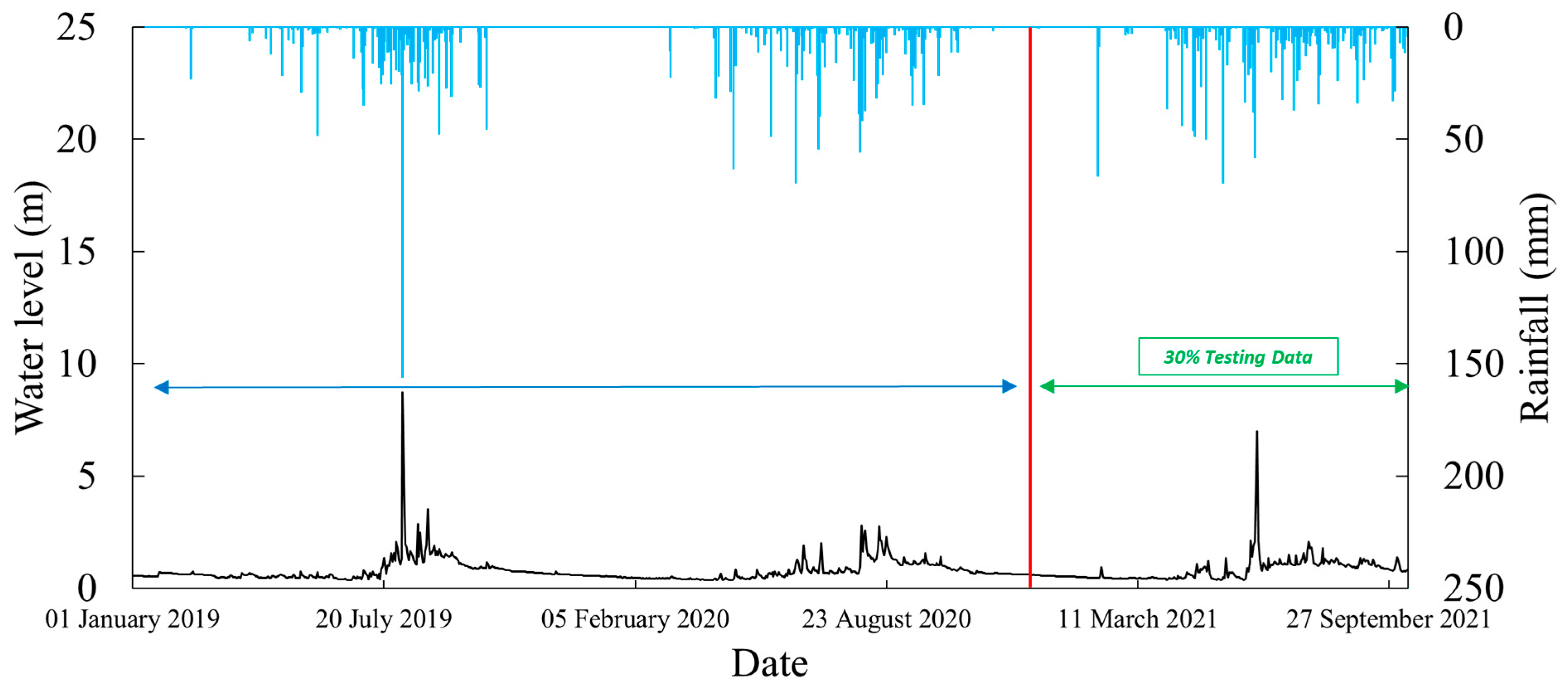
It is necessary to divide the collected data into two periods: training and testing. This is conducted for evaluating the efficiency of the trained LSTM models through modeling using the data in training and testing periods separately. The trained model is then diagnosed as to whether it is suffering from under-fitting or over-fitting by performing the simulations in training and testing periods. In this study, we have established that the first 70% of the data were used for training the model, while the remaining 30% of the data were adopted for testing purposes. Figure 4 illustrates an example of separating the data for into training and testing periods for the Phiangluang station. The first 70% of the collected data, which are from 01 January 2019 to 14 December 2020, have been used as the training data, while the remaining 30% of the data (which are from 15 December 2020 to 14 December 2021) have been applied as the testing data. The same ratio has been applied to separate the data in each respective station.

3.5. Architectures and Hyper-Parameters of LSTM Model

In order to design the structure of an LSTM model and to implement the established model, various parameter values must be specified. The parameters of the LSTM layer include the number of nodes, the return sequences, the activation function, and the input form of the data. In this study, an LSTM model with a series structure has been constructed in which one layer is connected to the next layer. This structure is called a sequential structure and is the most common structure adopted when designing a deep learning network for the first time.

The number of nodes informs the number of weights that can be recognized in the network. As the number of nodes increases, the model is more capable of recognizing complex patterns, but at the same time, the difficulty of learning will also be increasing. Moreover, if the number of data are insufficient, the model with a high number of nodes may also not be able to yield an appropriate level of learning.

The return sequences can be configured as a process of reaching a value of True or False based on a sequence-to-sequence or sequence-to-one format. When connecting LSTM layers continuously, the sequence of data must be maintained in a sequence-to-sequence format.

In a neural network, the activation function is responsible for transforming the summed weighted input from the node into the activation of the node or output for that input. In other words, an activation function is a function that limits or transforms the output of the network layer to a certain range. The rectified linear activation function (ReLU) applied in this study will output the input directly if the input is positive; otherwise, it will produce a value of zero. The ReLU function does not have a large computation cost and is simple to implement, so it has the advantage of a faster learning rate than the sigmoid function and the hyperbolic tangent function.

Most deep learning models are equipped with optimization tools and loss functions to optimize and further improve its learning ability and model efficiency. In this study, ADAM was used as the optimization function for hyper-parameter tuning, and MSE (mean square error) was used as the loss function to optimize the LSTM model established for water level prediction.

The fit function in Python was utilized to train the model in this study. It is necessary to specify the independent variables and the dependent variables in the fit function. Apart from that, it is also required to specify the number of times that the model will learn repeatedly through the epoch’s parameter. Last but not least, the batch size also has to be decided to allow for separating the training data whereby some portions of the training data will be allocated for validating the training model. The hyper-parameters adopted in this study are summarized in

Table 5. Adopted hyper-parameters in the LSTM model.

Parameters	Adopted Function/Value	Parameters	Adopted Function/Value
Activation Function	ReLU	Optimizer	ADAM
Loss Function	Mean Square Error	Batch Size	32
Epochs	60	Number of Nodes	64
Dropout	0.2	Learning Rate	0.0016

.

The architecture of the LSTM model applied in this study consists of an input layer, a hidden layer, and a dense layer that connects each input from the previous layer to each output neuron by providing learned linear transformations. The model is defined to have two inputs, rainfall and water level features, at the desired sequence length. The first hidden layer will be an LSTM layer with 64 units of neurons, and the output layer is a fully connected (dense) layer with a single neuron. Apart from that, the model is set to have a dropout rate of 0.2 to avoid the problem of over-fitting. Then, we fit the model with a run size of 60 epochs and a batch size of 32 for each sample, both in the training and testing datasets, with a learning rate of 0.0016. The architectures of the constructed LSTM model used in this study are also depicted in

Table 6. Summary of the architectures of the LSTM Model.

Model: “Sequential_5”
Layer (Type)	Output Shape	Parameters
lstm_5 (LSTM)	(None, 64)	17,152
dense_5 (dense)	(None, 1)	65
Total Parameters: 17,217
Trainable Parameters: 17,217
Non-trainable Parameters: 0

.

Only dynamic input data were used in training and testing the LSTM model in this study, which includes the daily point rainfall collected from nearby rainfall station and daily water level observed in respective water level station. The water levels recorded at particular previous time steps were also used as the dynamic input as it has been proven in previous studies [19,20] that the integration of previous water levels improved the forecasting performance of the LSTM model. These datasets were separated into training and testing datasets according to the criteria specified in the previous section. 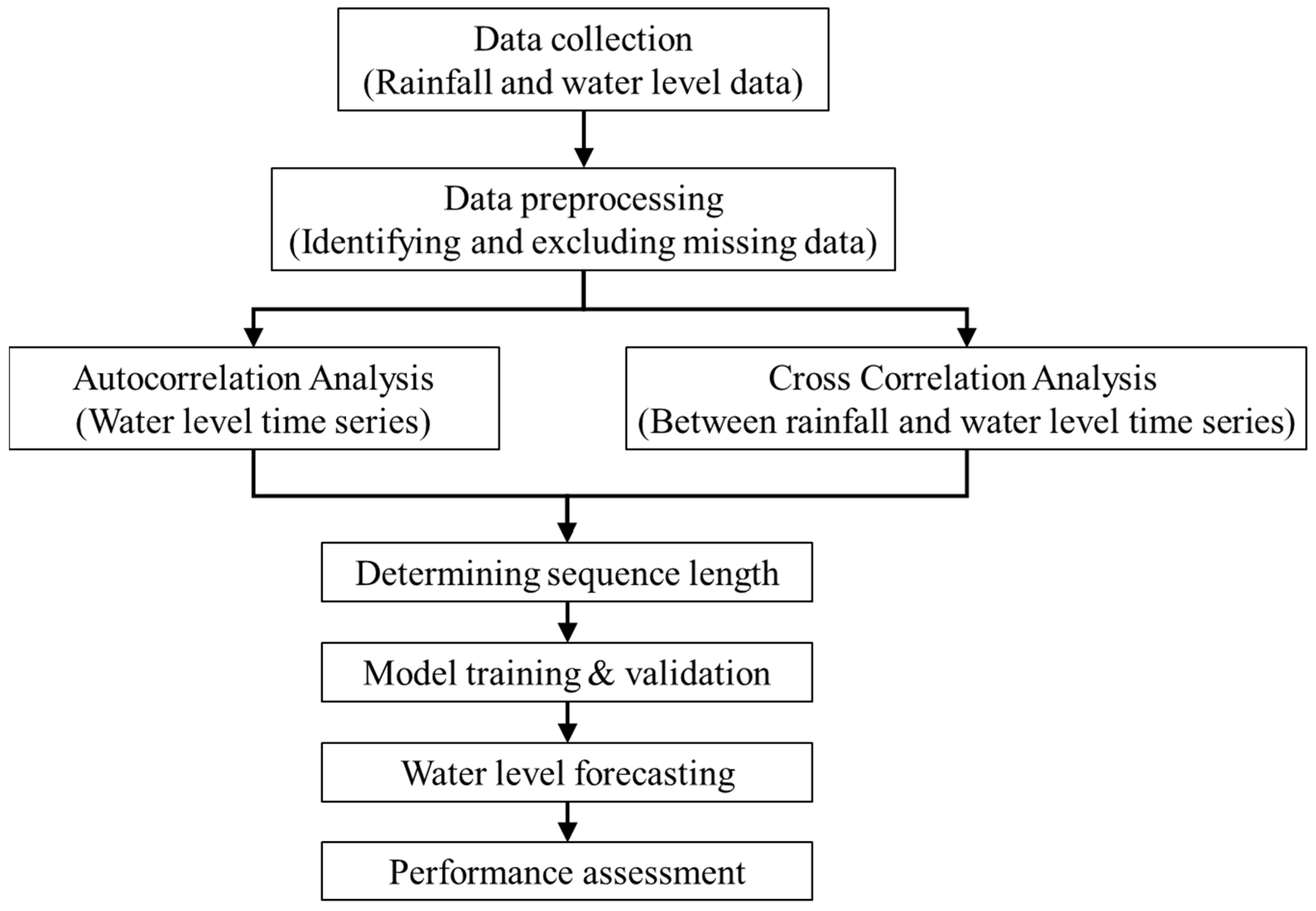Figure 5 depicts a flow chart summarizing the procedures involved in water level prediction and forecasting via the LSTM model used in this study.

3.6. Autocorrelation (acf) and Cross-Correlation (ccf)

The correlation relationship of a variable time series at current time step and its previous time step (lagged periods) is often obtained from a statistical analysis known as autocorrelation. In other words, autocorrelation analysis provides information about persistence of a variable by calculating the linear dependency of successive values over a given period [21]. The linear dependency is expressed in the range from −1 to 1, where a coefficient value close to 1 indicates a strong correlation. In this study, the water level time series is compared to itself with a discrete increase in lagged time/periods, and then the autocorrelation coefficient is calculated using Equations (2)–(4) [22].

$$A{C}_x\left(k\right)=\frac{C_x\left(k\right)}{C_x\left(0\right)}$$

(2)

$$C_x\left(k\right)=\frac{1}{N-k-1}{\displaystyle \sum _{i=1}^{N-k}\left(x_i-\overline{x}\right)}\left(x_{i+k}-\overline{x}\right)$$

(3)

$$C_x\left(0\right)=\frac{1}{N-k-1}{\displaystyle \sum _{i=1}^N{\left(x_i-\overline{x}\right)}^2}$$

(4)

where AC_x (k) represents the autocorrelation coefficient at lag time k, x is the cross-correlated time series (water level), $\overline{x}$ is the arithmetic mean of respective time series, N is the number of data, and C_x represents the auto-covariance. The graphical illustration of the cross-correlation coefficients calculated at each lag time is known as autocorrelogram.

While the correlation relationship between a similar time series shifted relatively in time is expressed as autocorrelation as presented in previous section, the correlation or comparison of two time series of different variables over a period of time can be obtained from the statistical method of cross-correlation. Similar to autocorrelation, the strength of correlation between the two time series variables at lagged periods is also expressed in range between −1 to 1, where positive values close to 1 indicate a strong correlation and negative values represent an anti/inverse correlation relationship. The cross-correlation between water level and rainfall in this study will be computed using Equations (5)–(7) [22], which are expressed as:

$$C{C}_{xy}\left(k\right)=\frac{C_{xy}\left(k\right)}{C_{xy}\left(0\right)}$$

(5)

$$C_{xy}\left(k\right)=\frac{1}{N-k-1}{\displaystyle \sum _{i=1}^{N-k}\left(x_i-\overline{x}\right)}\left(y_{i+k}-\overline{y}\right)$$

(6)

$$C_{xy}\left(0\right)=\frac{1}{N-k-1}{\displaystyle \sum _{i=1}^N\left(x_i-\overline{x}\right)}\left(y_i-\overline{y}\right)$$

(7)

where CCxy (k) represents the cross-correlation coefficient at lag time k, x and y are the cross-correlated time series (water level and rainfall), $\overline{x},\overline{y}$ are the arithmetic mean of the respective time series, N is the number of data in the respective time series, and C_xy represents the cross variance. The graphical illustration of the cross-correlation coefficients calculated at each lag time is also known as cross-correlogram.

The statsmodels Python library has been used to calculate the correlation coefficients of both autocorrelation and cross-correlation through the tsa.acf and tsa.stattools.ccf command functions. These correlation statistics will be used as the references for identifying the optimal sequence length to be adopted in the developed LSTM networks for predicting and forecasting water levels.

3.7. Performance Metrics of Predictions

The coefficient of determination (R²), root mean square error (RMSE), and Nash Sutcliffe Efficiency (NSE) have been adopted in this study as the indicators to verify the accuracy of the predicted results. As mentioned previously, each performance metric is described in Equations (8), (9), (10) and (11), respectively.

$$r_{OP}=\frac{{\displaystyle {\sum }_{i=1}^n(O_i-O^{\prime })(P_i-P^{\prime })}}{\sqrt{{\displaystyle {\sum }_{i=1}^n{(O_i-O^{\prime })}^2}}\sqrt{{\displaystyle {\sum }_{i=1}^n{(P_i-P^{\prime })}^2}}}$$

(8)

$$RMSE=\sqrt{\frac{{\displaystyle {\sum }_{i=1}^n{(O_i-P_i)}^2}}{n}}$$

(9)

$$R^2=\frac{{({\displaystyle {\sum }_{i=1}^n(O_i-O^{\prime })(P_i-P^{\prime })})}^2}{{\displaystyle {\sum }_{i=1}^n{(O_i-O^{\prime })}^2{\displaystyle {\sum }_{i=1}^n{(P_i-P^{\prime })}^2}}}$$

(10)

$$NSE=1-\frac{{\displaystyle {\sum }_{i=1}^n{(O_i-P_i)}^2}}{{\displaystyle {\sum }_{i=1}^n{(O_i-O^{\prime })}^2}}$$

(11)

R² is an indicator that can evaluate how well a predicted value can explain an observation. The range of R² is between 0 and 1, and the closer the value is to 1, the better the predicted value can explain the actual phenomenon. Here, O_i and P_i represent the observed and predicted values in i-interval, O′ represents the average of the observed values while P′ represents the average of the predicted values and n indicates the total number of datasets.

RMSE is an indicator that evaluates the error between predictions and observations. The range of the value is 0 to infinity. The closer the computed RMSE is to 0, the smaller the error and the closer the predictions are to the observations.

NSE is a widely used metric to evaluate the predictive performance of hydrological models. The closer the NSE value is to 1, the smaller the error between the observation and the prediction. If the NSE value is negative, it means that model’s predictions, which means that the predictions made by the model are inefficient.

4. Results and Discussions

4.1. Autocorrelation of Water Level Time Series

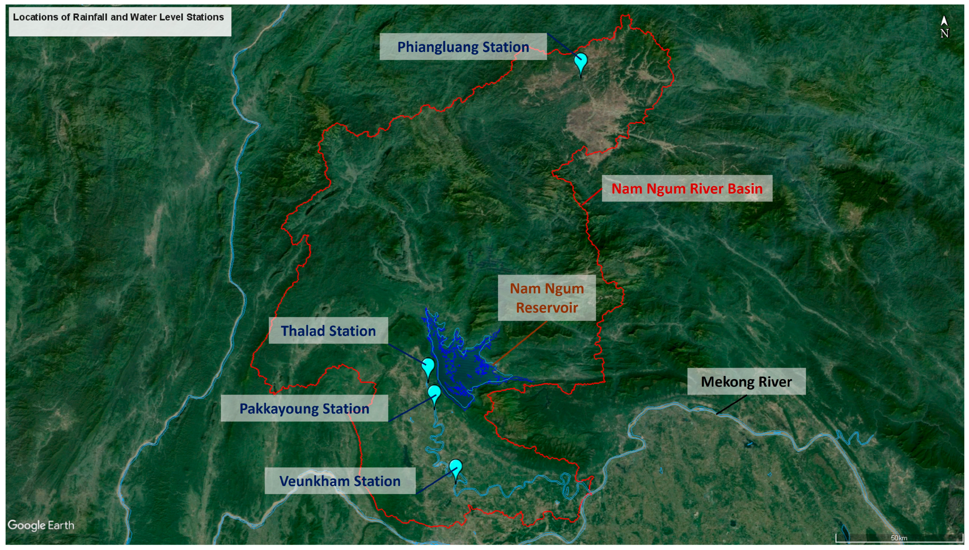
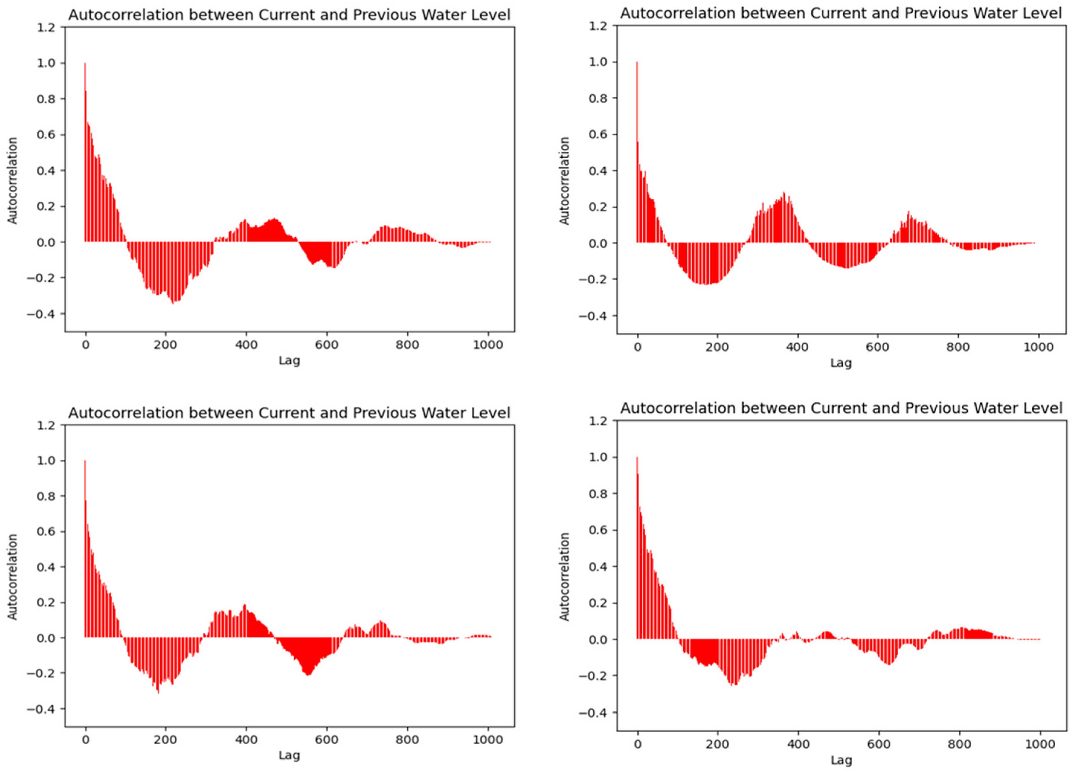
The autocorrelation coefficients estimated for the water level time series in the respective stations indicated that there is an extremely strong autocorrelation relationship, where the maximum coefficient values were all observed at a lag of 1 day with values of 0.924, 0.858, 0.951, and 0.729 in the stations Pakkayoung, Thalad, Veunkham, and Phiangluang, respectively. The autocorrelation coefficient was then decreased gradually as lag time increased until it achieved zero and negative values where the lag time was long enough that the water level at lag time t − n was no longer useful for influencing the water level at time t. It can also be observed from the autocorrelograms, as illustrated in Figure 6, that autocorrelation coefficients for water level time series actually behave like a cosine curve, whereby the values change repetitively from positive to negative and vice versa, and eventually become zero after several cycles.

This phenomenon could indicate that the daily water level is a non-random process that portrays high seasonal variability. Similar observations have also been found in previous studies [21,22,23]. According to Tigabu et al. [21], a strong autocorrelation has also been observed in the river discharge with its previous day’s discharge (Q_t−1) due to the storage effects of the previous day streamflow. Thus, since the river water level is also linearly proportional to the streamflow/discharge, it is not surprising that similar characteristics of autocorrelation for water level were obtained in this study.

Therefore, it is easier to predict or forecast the water level at the next time step based on the water level observed at the current time step as strong autocorrelation has been found at a lag of 1 day. Due to this reason, the water level observed at previous time steps was also used as the input for forecasting the water level at future steps in order to improve the performance of the LSTM model.

4.2. Cross-Correlation between Water Level and Rainfall Time Series

In classic hydrology, surface runoffs are believed to be generated from two mechanisms, namely infiltration excess and saturation excess. Both mechanisms share a similar concept that surface runoff will not be generated as soon as a storm is initiated; it will only be generated when the land surface is already saturated with water and the rainfall can no longer infiltrate the ground. Therefore, we typically observe there is a lag or delay between the rainfall hyetograph and streamflow/water level hydrograph. Thus, the concept of concentration time has been introduced in conceptual modeling to describe the delay between the rainfall and the generated surface runoff.

The concentration time of a river basin or watershed has traditionally been computed using empirical formulae based on the physical attributes of the watershed, such as the Kirpich Method. Currently, the relationship between the observed streamflow/water level in a river and rainfall can be assessed statistically by cross-correlating those time series over a given period.

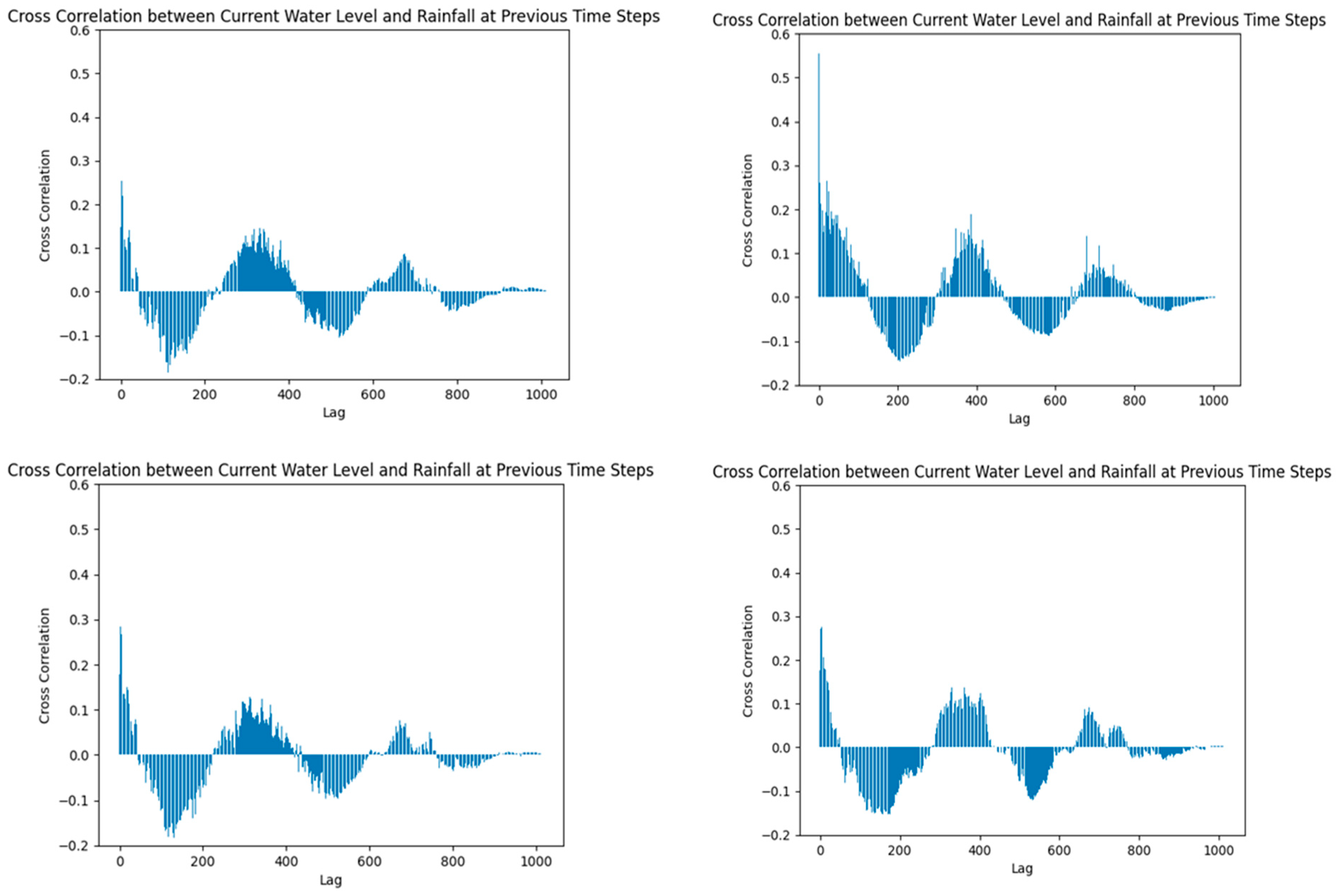
The cross-correlation (cc) coefficients between the water level and rainfall obtained for each respective station are illustrated in Figure 7. The Phiangluang station has been assigned with the maximum cc value of 0.555 at zero lag day, the Pakkayoung and Thalad stations have their highest cc values of 0.255 and 0.284 after 2 days of lag, and a maximum cc value of 0.278 after 3 days of lag has been found for the Veunkham station. According to Osman et al. [24], these positive correlation coefficients between rainfall and streamflow/water level with a lagging time are a signature of an autoregressive model. The cross-correlograms of water level and rainfall for each respective station, as illustrated in Figure 7, which is distinguished from conventional cross-correlograms as only half of the curves were portrayed in the diagrams where the conventional cross-correlograms often show the complete curves which include positive and negative lag/delay.

Usually, positive and negative lag/delay indicates the relative cross-correlation between two time series. For example, if a positive lag/delay represents the cross-correlation between current water level and rainfall at lagged steps, then negative lag/delay will automatically represent the cross-correlation between current rainfall and water level at lagged time steps. Since the current water level has been defined as an output and rainfall at lagged time steps are defined as input in the LSTM model, it is not necessary for us to understand the cross-correlation between the current rainfall and water level at lagged time steps. In fact, rainfall is not a dependent variable in the function of water level. Conversely, water level is a dependent variable in the function of rainfall. Therefore, only positive lag/delay values, which represent the cross-correlation between current water level and rainfall at lagged time steps, are plotted in Figure 6.

It has been established that the correlation between the water level and rainfall is not as strong as the autocorrelation observed in the water level time series. According to Wei et al. [23], the correlation degree for correlation coefficients between 0.4 and 0.6 is regarded as ‘Medium’, and ‘Weak’ correlation has been defined for correlation coefficients between 0.2 and 0.4. This shows that the rainfall would induce a smaller impact on the water level observed after n lag time. This phenomenon is believed to be caused by the fact that the contributing watershed areas at each water level station are very large, and only a point rainfall recorded at each respective rainfall station has been used to represent the relationship between the rainfall and water level, where point rainfall usually has limited spatial impacts over the whole watershed [22].

4.3. Determination of Sequence Length for LSTM Deep Learning Modeling

The results presented in the previous section have corroborated that the water level at the current time step does receive an impact in various degrees induced by the water level and rainfall at previous time steps. The sequence length, which is also known as the lookback period, is one of the important parameters that needs to be defined by the user before training an LSTM model. It determines the numbers of input data at a previous time step that will be used to simulate the output at the current time step.

An optimal sequence length will enable the developed LSTM model to be more efficient. Insufficient information of input data used for training which eventually results in the problem of under-fitting when too short a sequence length has been defined. Conversely, a long sequence length seems to guarantee sufficient information relating to the input data used for training, but it may eventually induce more noises and longer computation time is required for simulation.

In this study, we proposed to use the auto and cross-correlation coefficients to guide us in specifying the optimal sequence length in the LSTM model. It has been reported in Mangin [25] that a time series may lose its memory when a correlation coefficient value of less than 0.2 is computed at that particular lag time. In other words, the input data at that particular lag time are assumed to induce no impacts on the output at the current time.

Table 7. Lag time (day) required for correlation coefficient to drop beyond 0.2.

Stations	Lag Time (Day) Required for Correlation Coefficient to Drop beyond 0.2
	Autocorrelation (Water Level)	Cross-Correlation (Water Level and Rainfall)
Phiangluang	44	8
Pakkayoung	76	7
Thalad	69	7
Veunkham	76	9

summarizes the lag time required for the correlation coefficients of the water level and rainfall time series to drop beyond 0.2.

It can be seen in Table 6 that the autocorrelation coefficients (involving water level time series only) take longer time to drop beyond 0.2 where longest effective memory periods of 76 days were estimated for the stations Pakkayoung and Veunkham, followed by Thalad station (69 days), and shortest periods of 44 days were estimated for Phiangluang station. In contrast, shorter memory effects were observed in time series of water level and rainfall as the cross-correlation coefficients between these two time series only took lag time of single digit to drop beyond 0.2. The time series for the Pakkayoung and Thalad stations lost their memory in 7 days, 8 days were required for Phiangluang station, and the longest period of 9 days was consumed for Veunkham station.

This distinct difference is expected as the results of autocorrelation presented in previous section already informed that the water level time series was strongly auto-correlated with data at previous time steps while the cross-correlation between water level and rainfall at previous time steps was relatively weak. Adopting a long sequence length seems to be redundant as the results already confirmed that the major input for our LSTM model, rainfall time series had only short effective memory periods of about 7 to 9 days. Therefore, we propose to define the sequence length for training the LSTM model based on the effective memory periods obtained from the cross-correlation between water level and rainfall time series.

4.4. Training and Testing the LSTM Models

The LSTM model has been trained according to the architecture as presented in the previous section by using the water level and rainfall data obtained from four stations located in the Nam Ngum basin of Lao PDR. The model was trained for sequence lengths as suggested in Table 6 where each station has been assigned with an effective memory period based on the results concluded from autocorrelation and cross-correlation. For example, it has been estimated that the effective memory period for the Pakkayoung station is 7 days, so the training of the LSTM model for that station has been conducted from a sequence length ranging from 1 to 7 time steps, where each time step is equivalent to a one-day lagged period. The trained models have also been used to predict the water level output for the last 30% of the time series in the testing period to further validate the generalized capacity of these trained LSTM models

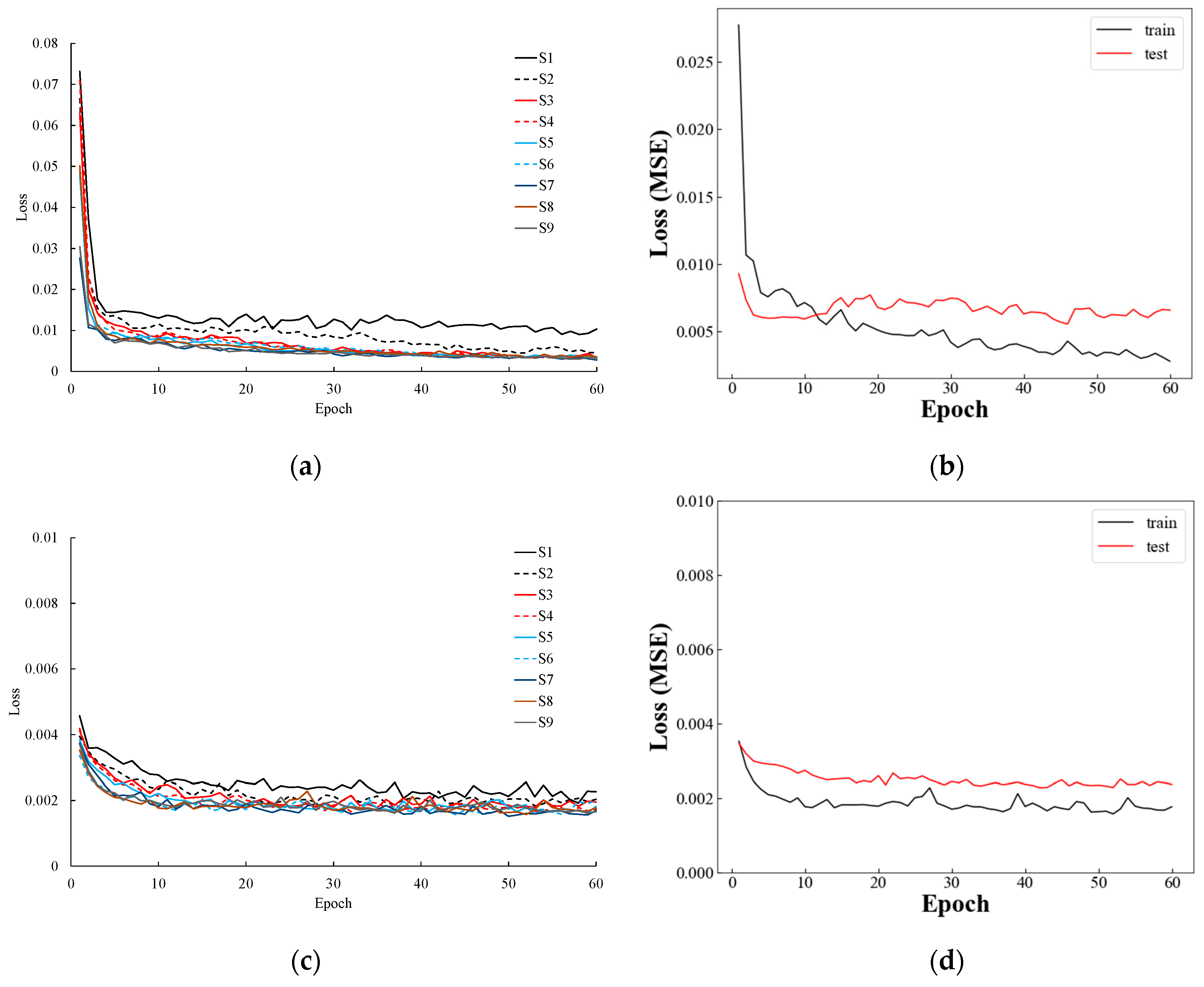
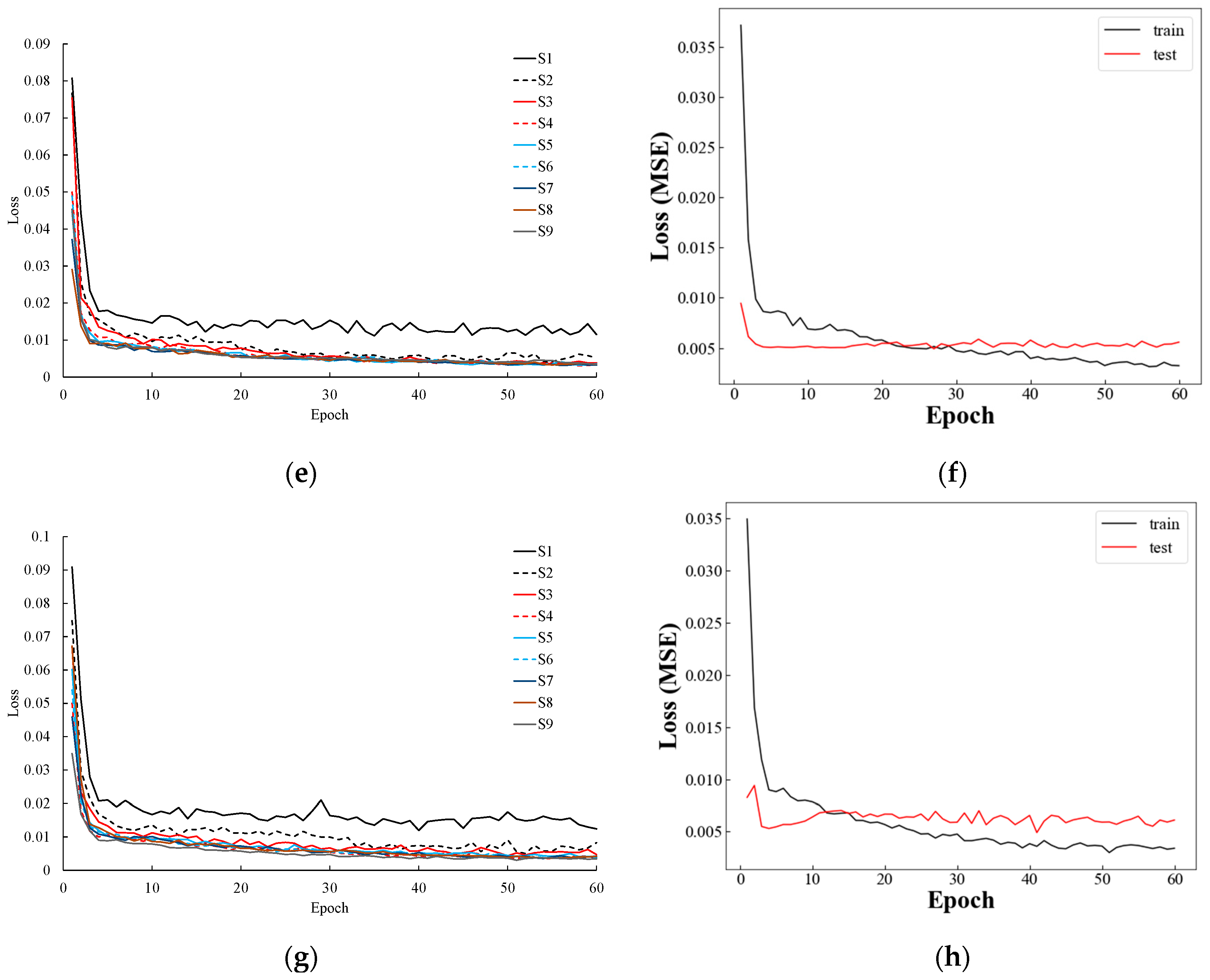
Figure 8 portrays the training and testing loss curves obtained from different sequence lengths, where the figures at the right-hand side indicate the training and testing loss curves in the effective memory periods estimated for each respective station. It can be observed from the figure that the training curves at a shorter sequence length (one and two lagged time steps) are always located at upper positions relative to the training curves of longer sequence lengths. This indicates that the prediction models of short sequence length seem to be inappropriate for the selected stations in the study area as training curves with greater errors/losses were obtained during the model training.

The hyper-parameter dropout, with a value of 0.2, was defined for the LSTM model, which controls the percentage of neurons to be dropped during the simulation with the aim of avoiding the problem of over-fitting. This dropout regularization has been adopted to achieve a better generalization of the trained models for data outside the training and testing sets. However, even though dropout regularization was applied during the model training, its loss was still lower than the testing loss. The gap between the training and testing loss curve was not significant. Thus, these trained models are believed to be appropriate for predicting and forecasting future water levels.

4.5. Model Validation

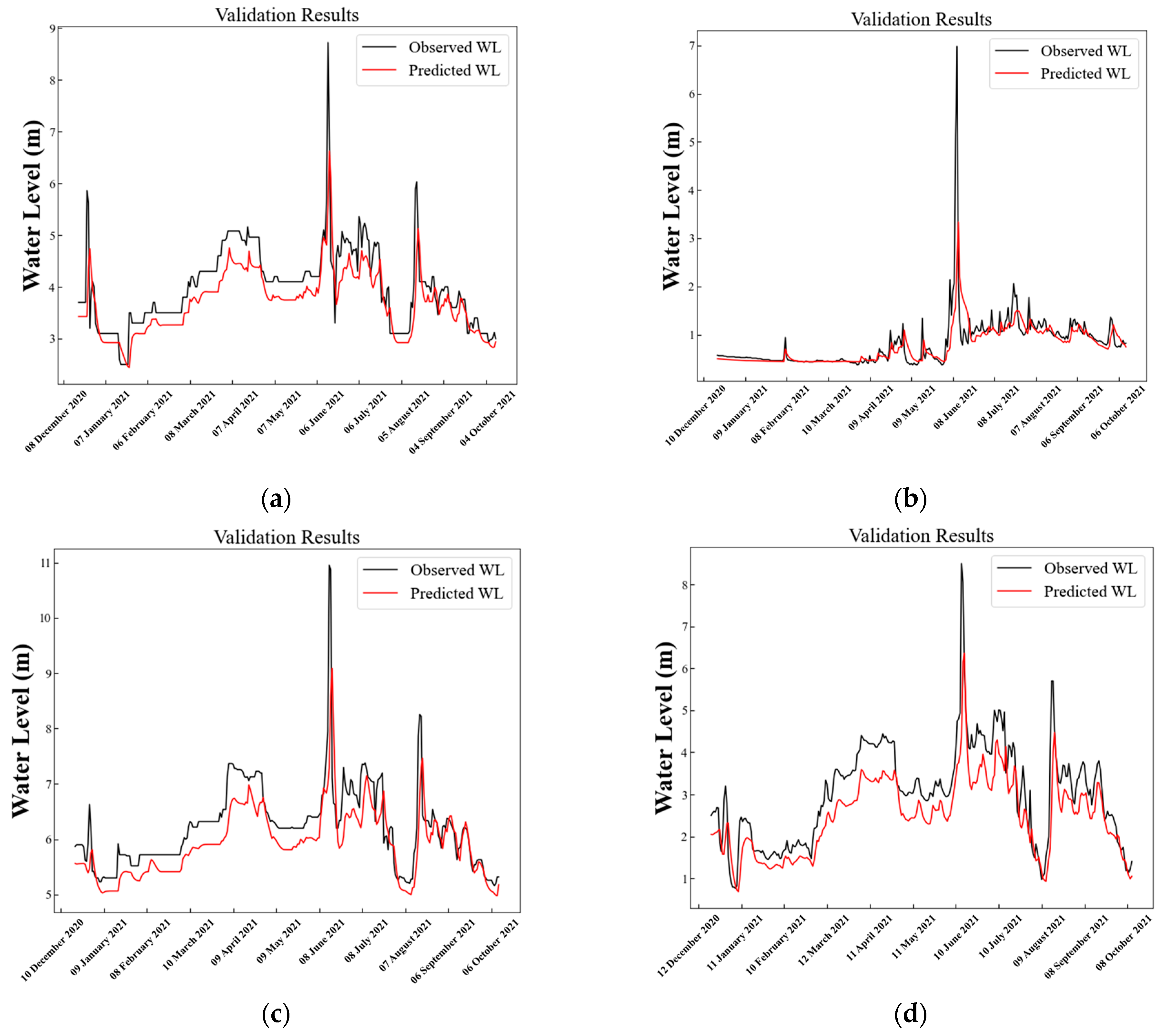
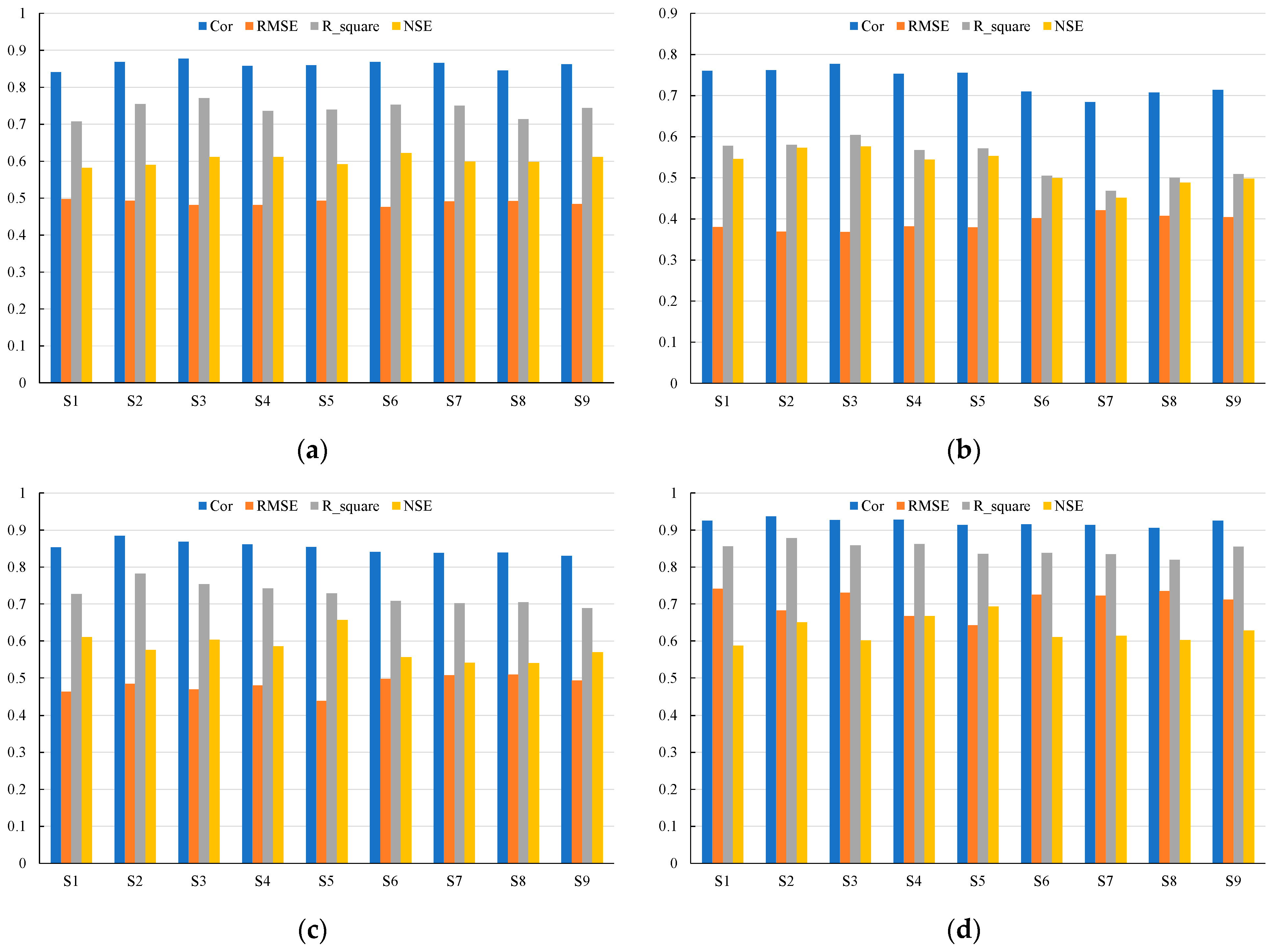
Figure 9 illustrates the validation of predicted and observed water level during the testing period at the sequence length of effective memory period and its performance metrics at different sequence lengths are also portrayed in Figure 10. It is found that most of the estimated NSE ranged between 0.5 and 0.7, except for the Phiangluang station, where the estimated NSE values were between 0.4 and 0.5 for a sequence length greater than 6. By having NSE values between 0.5 and 0.7, its prediction ability can be regarded as fair and good according to the reference values suggested for hydrological model performance provided in Hugo et al. [26], where NSE between 0.50 and 0.65 is regarded as ‘Fair’, NSE between 0.65 and 0.75 is regarded as ‘Good’, and NSE greater than 0.75 is considered to be ‘Very Good’. Any model which produces NSE less than 0.50 is recognized as inadequate.

It is also observed that high R² metric values have been obtained in most of the stations, ranging from 0.6 to 0.9, except for the Phiangluang station, where the estimated R² metric values were between 0.4 and 0.6. High R² metric values further indicated smaller differences between the observed data and predicted water level by LSTM model in the testing period. Apart from that, low RMSE metric values ranging from 0.37 to 0.74 were estimated for error evaluation between the predicted and observed water level. All statistical measures obtained from the LSTM model’s performance evaluation have pointed out that the trained LSTM model developed in this study can be considered as fair and adequate for water level prediction for each respective water level station located in the Nam Ngum River Basin.

However, we observed that there was an offset between the observed and predicted water level hydrographs in each station and the predicted peak water levels were always lower than the observed peak water levels. Constant hyper-parameters have been adopted to train the LSTM models at each respective water level station in this study as hyper-parameter optimization is not the main objective of this study. We have defined the hyper-parameters required for training the LSTM models by referring to the previous similar LSTM studies [20]. Thus, we admit that there is room to further improve the performance of the LSTM models in this study and we recognized that there is a need to optimize the hyper-parameters used to train the LSTM models. We believe that the problems of offset and low predicted peak water level can be resolved by fine tuning the models through parameter optimization.

Another interesting phenomenon has also been observed from the results of the performance metrics, whereby the stations located upstream saw their estimated NSE values peak at a shorter sequence length. Conversely, the stations located downstream achieved their peak NSE values at a longer sequence length. The Phiangluang station is located upstream of the Nam Ngum River and reached its peak NSE of 0.576 at a sequence length of 3, while the Pakkayoung, Thalad, and Veunkham stations are located downstream of the Nam Ngum River, achieving their peak NSE of 0.622, 0.657, and 0.693 at a longer sequence length of 6, 5, and 5, respectively. Again, this observation is consistent with the concept of concentration time where the upstream basins usually have a shorter concentration time than those basins located downstream.

4.6. Forecasting Using the Trained Model

The trained LSTM models have been used to ‘forecast’ water levels (at the respective stations) for selected storms that occurred in the past to validate their practicability in flood forecasting. The water level forecasting was dependent on the sequence length defined during the training stage of the LSTM models. For example, five forecasted water levels at t + 1 to t + 5 will be produced when a sequence length of 5 is used in training the models. Five input datasets from t to t − 4 are required to forecast the water level at time t + 1, where t represents time of present/current and t + 1 represents one future time step. Consequently, the water level at t + 2 is forecasted based again on five input datasets from t − 3 to t + 1. This process will be iterated until the water level at t + 5 is obtained. Since the target variable water levels at previous time steps will be used as the input data for predicting the water levels at the next time step, the forecasted water levels will also be used to forecast the water levels at the next time step. In other words, the forecasted water level at t + 5 will be based on the forecasted water level from t + 1 to t + 4, the current water level at t, and the rainfall data from t to t + 4.

The effects of sequence length become more prominent for forecasting the water level in future. The forecasted water level will not be accurate if sequence length is not properly defined in the trained LSTM model. For instance, a forecasted water level will not rise if the defined sequence length is too short. Supposing that the water level should rise at current time step, t, due to the storms that occurred at the five previous time steps, t − 5. However, if we define the LSTM model to have 1 sequence length, it will only train the model and forecast based on the storm occurred at a previous time step, t − 1. If there is no storm that occurred at a time step of t − 1, the forecasted water level will not rise in accordance with expectations, and it will eventually lead to missed alerts and warnings. In fact, it has been reported in some previous studies that the sequence length did affect the simulation of streamflow using LSTM for rainfall runoff modeling. Kratzert et al. [27] mentioned that the time steps influencing the LSTM model’s input data were dynamic, whereby they decreased during dry periods with high temperatures and increased during wet periods with relatively lower temperatures.

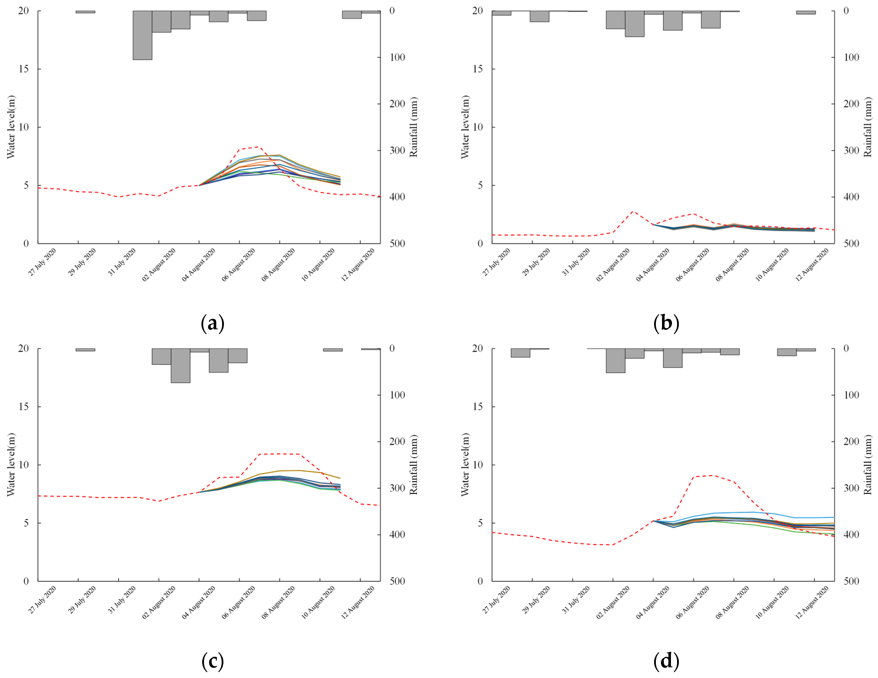
Figure 11 shows the comparison of the forecasted water level hydrographs (colored solid lines) with the observed water level hydrographs (red dotted lines) at effective memory periods in respective stations for a storm that occurred in early August 2020. The forecasting has been carried out for 10 iterations to monitor the effects of the LSTM model stochasticity on the forecasted water level. It is apparent that the forecasted water level hydrographs for the Pakkayoung station generally corresponded with the observed water level hydrograph, whereby the forecasted water levels rose accordingly with respect to the storms that occurred at previous time steps. The forecasted water level in the Thalad station also rose as per expectations, but the rising magnitude was lower than expectations. However, the forecasted water level hydrographs for the Phiangluang and Veunkham stations deviated from the observed ones.

Table 8. Forecasting performance at Pakkayoung station at different sequence lengths.

Sequence Length	3	4	5	6	7	8	9
Correlation Coefficient	0.987	0.968	0.691	0.605	0.711	0.95	0.91
RMSE	3.079	3.116	2.908	2.675	2.421	2.373	2.139
R2	0.975	0.937	0.477	0.366	0.506	0.903	0.828
NSE	−2.603	−3.726	−3.4	−1.879	−0.882	−0.57	−0.161

,

Table 9. Forecasting performance at Phiangluang station at different sequence lengths.

Sequence Length	3	4	5	6	7	8	9
Correlation Coefficient	0.703	−0.348	−0.431	−0.141	−0.022	0.424	0.533
RMSE	0.677	0.659	0.661	0.599	0.557	0.537	0.506
R2	0.494	0.121	0.186	0.02	0.001	0.18	0.284
NSE	−3.395	−1.41	−1.41	−0.997	−0.643	−0.578	−0.347

,

Table 10. Forecasting performance at Thalad station at different sequence lengths.

Sequence Length	3	4	5	6	7	8	9
Correlation Coefficient	0.878	0.906	0.918	0.898	0.861	0.959	0.98
RMSE	1.518	1.699	1.787	1.626	1.539	1.54	1.406
R2	0.771	0.821	0.843	0.806	0.742	0.92	0.961
NSE	−1.644	−1.899	−2.359	−2.123	−0.648	−0.044	0.289

and

Table 11. Forecasting performance at Veunkham station at different sequence lengths.

Sequence Length	3	4	5	6	7	8	9
Correlation Coefficient	0.987	0.968	0.691	0.605	0.711	0.95	0.91
RMSE	3.079	3.116	2.908	2.675	2.421	2.373	2.139
R2	0.975	0.937	0.477	0.366	0.506	0.903	0.828
NSE	−2.603	−3.726	−3.4	−1.879	−0.882	−0.57	−0.161

summarize the performance metrics of forecasting at different sequence lengths. We can observe from this statistic that the forecasting performance improved at the sequence length of effective memory periods in the respective stations. It is found that the highest NSE and lowest RMSE values are achieved for the trained models at or after the sequence length of effective memory periods defined in the respective stations. This proves the feasibility of our proposal to define the optimal sequence length for forecasting in an LSTM model based on autocorrelation and cross-correlation analysis between rainfall and water level time series, as explained in Section 4.3.

5. Conclusions

Water level prediction and forecasting have been established using an LSTM model for four water level stations located along the Nam Ngum River in the Nam Ngum River Basin, Laos PDR. The correlation between input and output data has also been examined through the analysis of autocorrelation and cross-correlation. It was found that the water level time series in the study area was a strong autoregressive model, whereby the water level at current time step was strongly correlated to its water level recorded at previous time steps. Positive correlation coefficients were also computed for cross-correlation between the rainfall and water level time series, which again shows that it was an autoregressive model. However, the magnitude or power of the autoregressive model was not as strong as observed in water level time series. It is therefore proposed that the optimal sequence length to be applied in the modeling be defined based on the threshold of correlation coefficients obtained from water levels and rainfall in the respective stations, whereby there will be no correlation between two variables at particular time steps when the correlation coefficient is less than 0.2. It is found that the effective memory periods for the water level and rainfall time series collected from the selected stations in this study ranged from about 7 to 9 previous time steps (days), which indicated that the autocorrelation and cross-correlation analysis did help in determining the optimal sequence length in the LSTM model. By performing simulations with constant hyper-parameters and an optimal sequence length, the trained LSTM models in this study can be considered as fair and adequate for water level prediction for each respective water level station located in the Nam Ngum River Basin, as NSE values from 0.5 to 0.7 were mostly obtained from the model validations in the testing periods. The performance levels of the LSTM model in forecasting water levels in future periods varied in the Nam Ngum River Basin: the forecasted water level hydrographs for the Pakkayoung station generally corresponded with the observed water level hydrograph, whereby the forecasted water levels rose in accordance with the storms that occurred at previous time steps in early August 2020; however, the forecasted water level hydrographs produced from the trained LSTM models for other stations deviated quite significantly from the observed ones.

It is important to mention that there is room to further improve the performance of the LSTM models established in this study. For example, we noticed that there were offsets between the predicted/forecasted water level and observed water level, and we believe that this problem can be resolved by fine-tuning the models through parameter optimization. Currently, we are working on writing the codes that integrate LSTM modeling and hyper-parameter optimization, and we expect to publish the new findings in upcoming papers. In addition, the LSTM model seems to require data from longer time periods to achieve better interpretations of the embedded relationship between the input and output data. Securing additional data in the future may improve the forecasting ability of the LSTM model. Last but not least, it is beneficial to increase the dimension of input data by integrating other significant meteorological variables such as evapotranspiration. Another prominent hidden relationship between the input and output data may be discovered by increasing the dimension of input data, and in doing so, the performance of the LSTM model may eventually be further improved.