

Water Distribution Network Partitioning Based on Complex Network Theory: The Udine Case Study


Abstract
1. Introduction
2. Materials and Methods
2.1. Clustering
- Intracluster edges: ;
- Intercluster edges:
- Clustering quality indices:
- Hydraulic indices:
2.2. Water Network Dividing
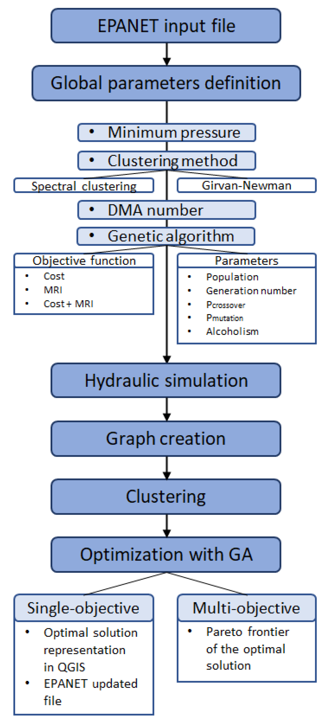
2.3. Methodology
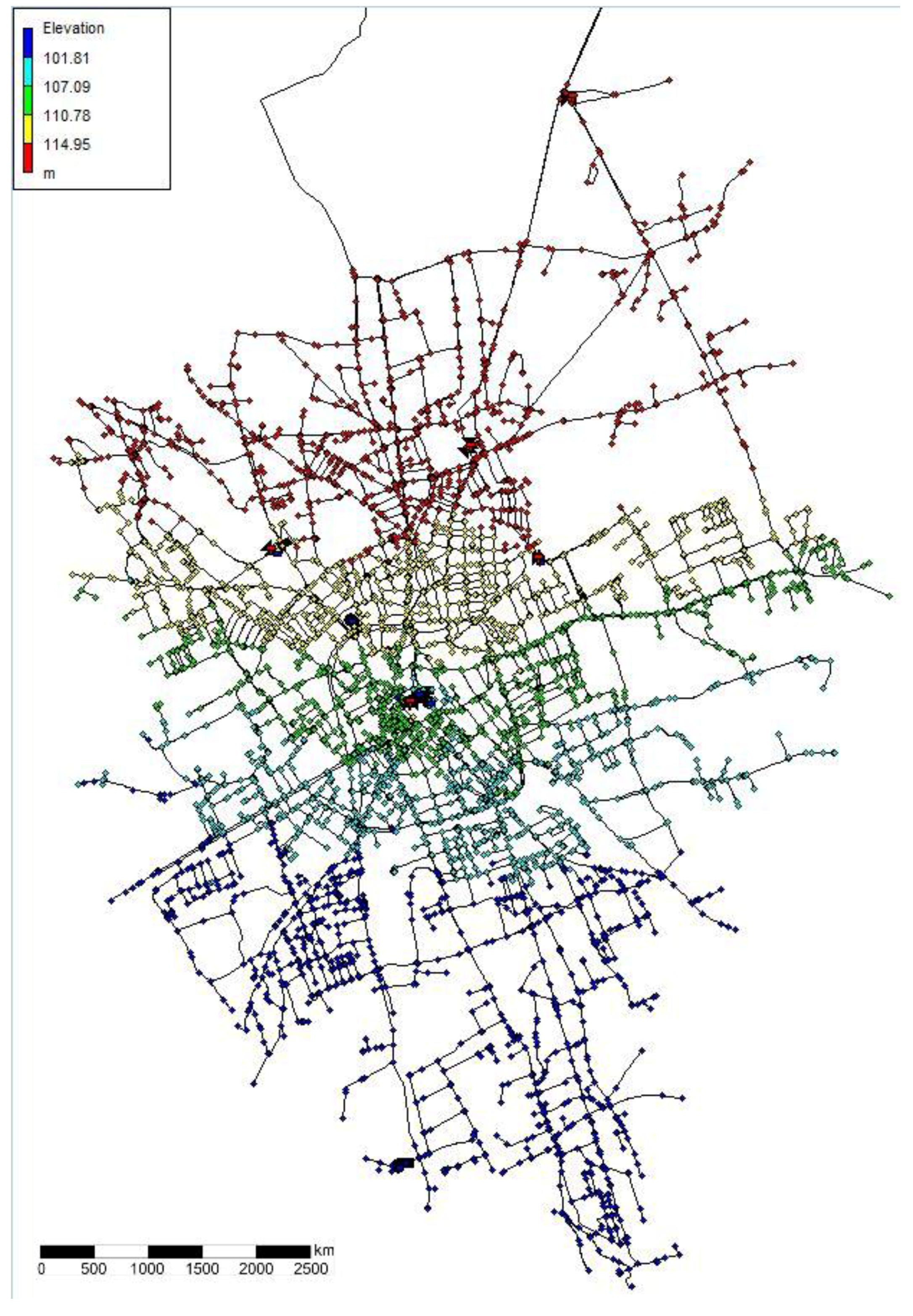
3. Results
- n = 5793 nodes;
- m = 6466 pipes;
- Six sources;
- Five tanks;
- Five pumps.
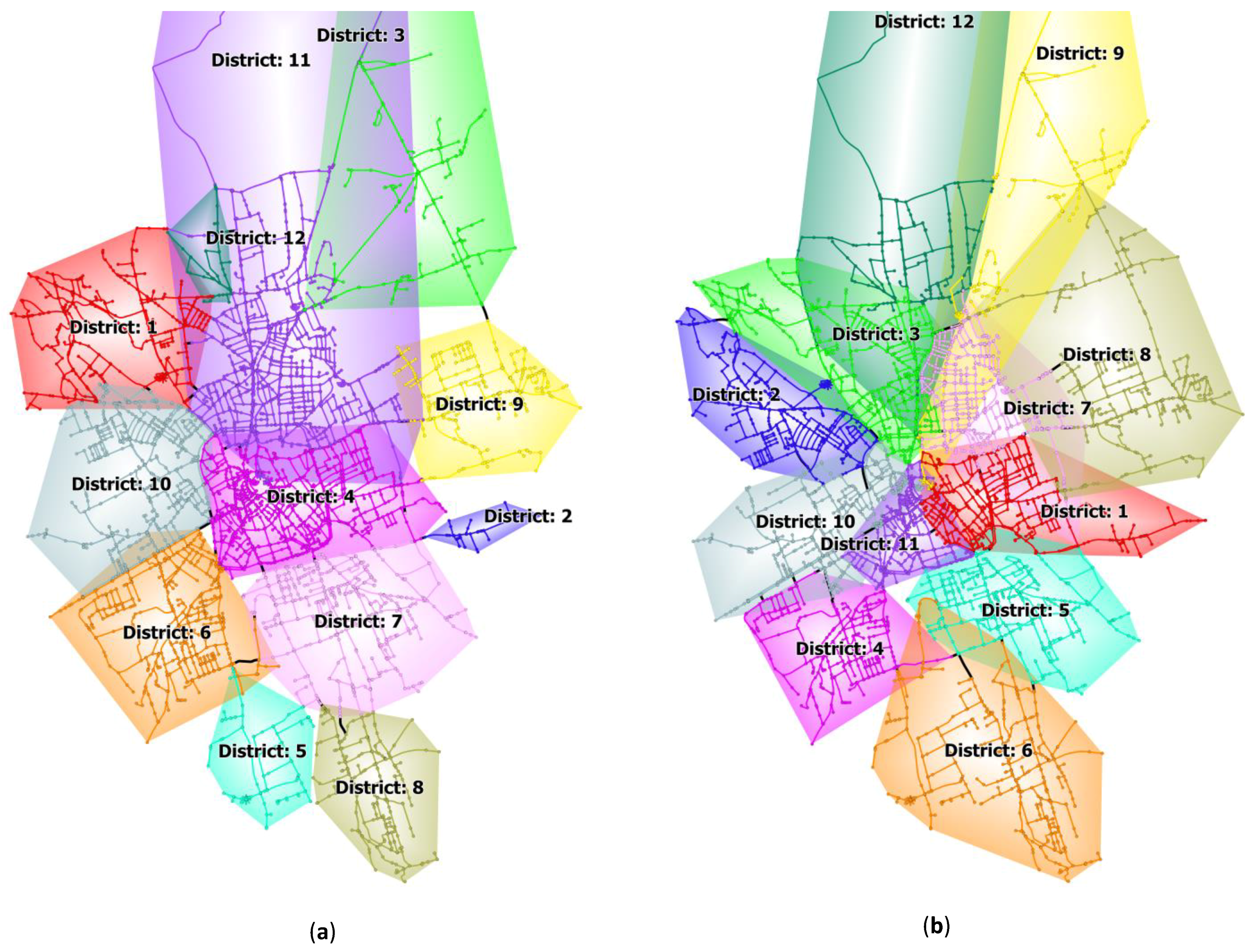
3.1. Clustering Analysis
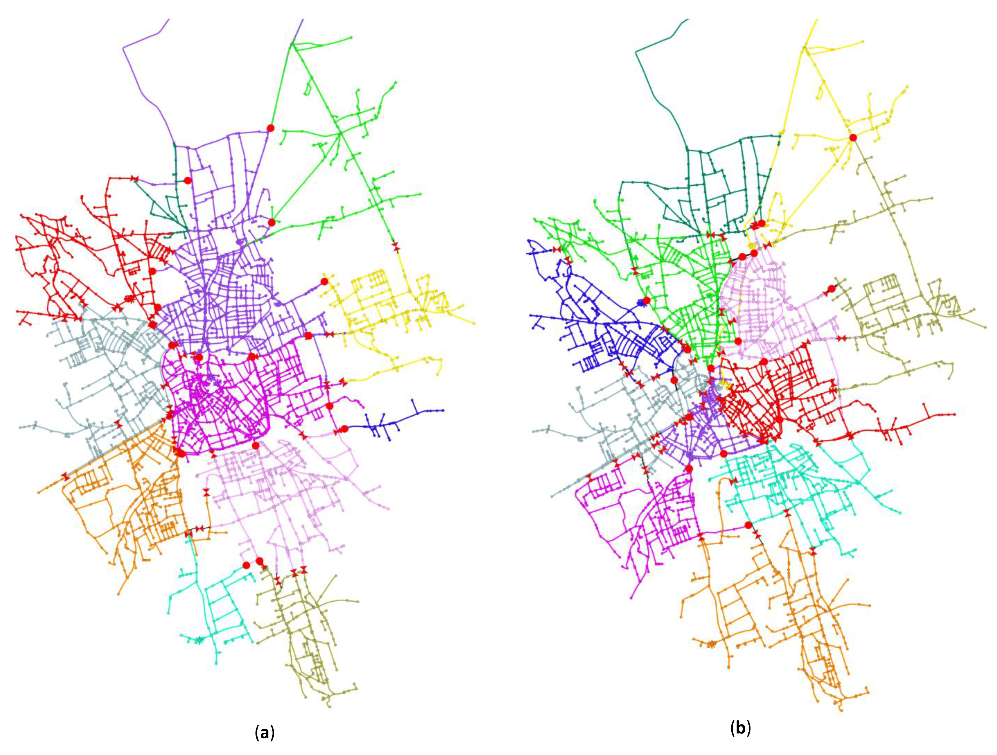
3.2. Dividing Phase
- Individuals = 150;
- Generations = 150.
- Tournament selection with tournament dimension equal to two for the single-objective optimization;
- Elitist non-dominated sorting genetic algorithm (NSGA-II) for the multi-objective function;
- Two-point crossover with crossover probability (;
- Flip-bit mutation with individual mutation probability and gene mutation probability .
4. Conclusions
Author Contributions
Funding
Data Availability Statement
Conflicts of Interest
References
- Saldarriaga, J.; Bohorquez, J.; Celeita, D.; Vega, L.; Paez, D.; Savic, D.; Dandy, G.; Filion, Y.; Grayman, W.; Kapelan, Z. Battle of the Water Networks District Metered Areas. J. Water Resour. Plan. Manag. 2019, 145, 04019002. [Google Scholar] [CrossRef]
- Morrison, J.; Tooms, S.; Rogers, D. DMA Management Guidance Notes; IWA Publishing: London, UK, 2007. [Google Scholar]
- Di Nardo, A.; Di Natale, M.; Santonastaso, G.F.; Tzatchkov, V.G.; Alcocer-Yamanaka, V.H. Water Network Sectorization Based on Graph Theory and Energy Performance Indices. J. Water Resour. Plan. Manag. 2014, 140, 620–629. [Google Scholar] [CrossRef]
- Walski, T.M.; Chase, D.V.; Savic, D.A.; Grayman, W.; Beckwith, S.; Koelle, E. Advanced Water Distribution Modelling and Management; Haestad Press: Waterbury, CT, USA, 2003. [Google Scholar]
- Alvisi, S.; Franchini, M. A Procedure for the Design of District Metered Areas in Water Distribution Systems. Procedia Eng. 2014, 70, 41–50. [Google Scholar] [CrossRef]
- Scarpa, F.; Lobba, A.; Becciu, G. Elementary DMA Design of Looped Water Distribution Networks with Multiple Sources. J. Water Resour. Plan. Manag. 2016, 142, 04016011. [Google Scholar] [CrossRef]
- Sela Perelman, L.; Allen, M.; Preis, A.; Iqbal, M.; Whittle, A.J. Automated Sub-Zoning of Water Distribution Systems. Environ. Model. Softw. 2015, 65, 1–14. [Google Scholar] [CrossRef]
- Tzatchkov, V.G.; Alcocer-Yamanaka, V.H.; Bourguett Ortíz, V. Graph Theory Based Algorithms for Water Distribution Network Sectorization Projects. In Water Distribution Systems Analysis Symposium 2006; American Society of Civil Engineers: Cincinnati, OH, USA, 2008; pp. 1–15. [Google Scholar]
- Perelman, L.; Ostfeld, A. Topological Clustering for Water Distribution Systems Analysis. Environ. Model. Softw. 2011, 26, 969–972. [Google Scholar] [CrossRef]
- Diao, K.; Zhou, Y.; Rauch, W. Automated Creation of District Metered Area Boundaries in Water Distribution Systems. J. Water Resour. Plan. Manag. 2013, 139, 184–190. [Google Scholar] [CrossRef]
- Campbell, E.; Ayala-Cabrera, D.; Izquierdo, J.; Pérez-García, R.; Tavera, M. Water Supply Network Sectorization Based on Social Networks Community Detection Algorithms. Procedia Eng. 2014, 89, 1208–1215. [Google Scholar] [CrossRef]
- Ciaponi, C.; Murari, E.; Todeschini, S. Modularity-Based Procedure for Partitioning Water Distribution Systems into Independent Districts. Water Resour. Manag. 2016, 30, 2021–2036. [Google Scholar] [CrossRef]
- Di Nardo, A.; Di Natale, M.; Giudicianni, C.; Musmarra, D.; Santonastaso, G.F.; Simone, A. Water Distribution System Clustering and Partitioning Based on Social Network Algorithms. Procedia Eng. 2015, 119, 196–205. [Google Scholar] [CrossRef]
- Giustolisi, O.; Ridolfi, L. New Modularity-Based Approach to Segmentation of Water Distribution Networks. J. Hydraul. Eng. 2014, 140, 04014049. [Google Scholar] [CrossRef]
- Zhang, Q.; Wu, Z.Y.; Zhao, M.; Qi, J.; Huang, Y.; Zhao, H. Automatic Partitioning of Water Distribution Networks Using Multiscale Community Detection and Multiobjective Optimization. J. Water Resour. Plan. Manag. 2017, 143, 04017057. [Google Scholar] [CrossRef]
- Brentan, B.M.; Campbell, E.; Meirelles, G.L.; Luvizotto, E.; Izquierdo, J. Social Network Community Detection for DMA Creation: Criteria Analysis through Multilevel Optimization. Math. Probl. Eng. 2017, 2017, 9053238. [Google Scholar] [CrossRef]
- Brentan, B.; Campbell, E.; Goulart, T.; Manzi, D.; Meirelles, G.; Herrera, M.; Izquierdo, J.; Luvizotto, E. Social Network Community Detection and Hybrid Optimization for Dividing Water Supply into District Metered Areas. J. Water Resour. Plan. Manag. 2018, 144, 04018020. [Google Scholar] [CrossRef]
- Di Nardo, A.; Di Natale, M.; Santonastaso, G.F.; Venticinque, S. An Automated Tool for SmartWater Network Partitioning. Water Resour. Manag. 2013, 27, 4493–4508. [Google Scholar] [CrossRef]
- Alvisi, S. A New Procedure for Optimal Design of District Metered Areas Based on the Multilevel Balancing and Refinement Algorithm. Water Resour. Manag. 2015, 29, 4397–4409. [Google Scholar] [CrossRef]
- Di Nardo, A.; Di Natale, M.; Giudicianni, C.; Greco, R.; Santonastaso, G.F. Weighted Spectral Clustering for Water Distribution Network Partitioning. Appl. Netw. Sci. 2017, 2, 19. [Google Scholar] [CrossRef]
- Liu, J.; Han, R. Spectral Clustering and Multicriteria Decision for Design of District Metered Areas. J. Water Resour. Plan. Manag. 2018, 144, 04018013. [Google Scholar] [CrossRef]
- Di Nardo, A.; Giudicianni, C.; Greco, R.; Herrera, M.; Santonastaso, G. Applications of Graph Spectral Techniques to Water Distribution Network Management. Water 2018, 10, 45. [Google Scholar] [CrossRef]
- Izquierdo, J.; Herrera, M.; Montalvo, I.; Pérez-García, R. Division of Water Distribution Systems into District Metered Areas Using a Multi-Agent Based Approach. Commun. Comput. Inf. Sci. 2011, 50, 167–180. [Google Scholar]
- Hajebi, S.; Barrett, S.; Clarke, A.; Clarke, S. Multi-agent simulation to support water distribution network partitioning. In Proceedings of the Modelling and Simulation 2013-European Simulation and Modelling Conference, ESM 2013, (Fernández), Lancaster, UK, 23–25 October 2013; pp. 163–168. [Google Scholar]
- Herrera, M.; Izquierdo, J.; Pérez-García, R.; Montalvo, I. Multi-Agent Adaptive Boosting on Semi-Supervised Water Supply Clusters. Adv. Eng. Softw. 2012, 50, 131–136. [Google Scholar] [CrossRef]
- Khoa Bui, X.; Marlim, M.S.; Kang, D. Water Network Partitioning into District Metered Areas: A State-Of-The-Art Review. Water 2020, 12, 1002. [Google Scholar] [CrossRef]
- Giudicianni, C.; Herrera, M.; di Nardo, A.; Adeyeye, K. Automatic Multiscale Approach for Water Networks Partitioning into Dynamic District Metered Areas. Water Resour. Manag. 2020, 34, 835–848. [Google Scholar] [CrossRef]
- Alvisi, S.; Franchini, M. A Heuristic Procedure for the Automatic Creation of District Metered Areas in Water Distribution Systems. Urban Water J. 2014, 11, 137–159. [Google Scholar] [CrossRef]
- Gomes, R.; Marques, A.S.A.; Sousa, J. District Metered Areas Design Under Di_erent Decision Makers’ Options: Cost Analysis. Water Resour. Manag. 2013, 27, 4527–4543. [Google Scholar] [CrossRef]
- Di Nardo, A.; Di Natale, M.; Giudicianni, C.; Santonastaso, G.; Tzatchkov, V.; Varela, J. Economic and Energy Criteria for District Meter Areas Design of Water Distribution Networks. Water 2017, 9, 463. [Google Scholar] [CrossRef]
- Di Nardo, A.; Di Natale, M.; Santonastaso, G.F.; Tzatchkov, V.G.; Alcocer-Yamanaka, V.H. Water Network Sectorization Based on a Genetic Algorithm and Minimum Dissipated Power Paths. Water Sci. Technol. Water Supply 2013, 13, 951–957. [Google Scholar] [CrossRef]
- Shao, Y.; Yao, H.; Zhang, T.; Chu, S.; Optimal, X. An Improved Genetic Algorithm for Optimal Layout of Flow Meters and Valves in Water Network Partitioning. Water 2019, 11, 1087. [Google Scholar] [CrossRef]
- Zhang, K.; Yan, H.; Zeng, H.; Xin, K.; Tao, T. A Practical Multi-Objective Optimization Sectorization Method for Water Distribution Network. Sci. Total Environ. 2019, 656, 1401–1412. [Google Scholar] [CrossRef]
- De Paola, F.; Fontana, N.; Galdiero, E.; Giugni, M.; Savic, D.; Degli Uberti, G.S. Automatic Multi-Objective Sectorization of a Water Distribution Network. Procedia Eng. 2014, 89, 1200–1207. [Google Scholar] [CrossRef]
- Hajebi, S.; Temate, S.; Barrett, S.; Clarke, A.; Clarke, S. Water Distribution Network Sectorisation Using Structural Graph Partitioning and Multi-Objective Optimization. Procedia Eng. 2014, 89, 1144–1151. [Google Scholar] [CrossRef]
- Giudicianni, C.; Herrera, M.; di Nardo, A.; Carravetta, A.; Ramos, H.M.; Adeyeye, K. Zero-Net Energy Management for the Monitoring and Control of Dynamically-Partitioned Smart Water Systems. J. Clean. Prod. 2020, 252, 119745. [Google Scholar] [CrossRef]
- Deb, K.; Agrawal, S.; Pratap, A.; Meyarivan, T. A Fast Elitist Non-Dominated Sorting Genetic Algorithm for Multi-Objective Optimization: NSGA-II. In Parallel Problem Solving from Nature PPSN VI; Schoenauer, M., Deb, K., Rudolph, G., Yao, X., Lutton, E., Merelo, J.J., Schwefel, H.-P., Eds.; Springer: Berlin/Heidelberg, Germany, 2000; Volume 1917, pp. 849–858. [Google Scholar]
- Campbell, E.; Izquierdo, J.; Montalvo, I.; Pérez-García, R. A Novel Water Supply Network Sectorization Methodology Based on a Complete Economic Analysis, Including Uncertainties. Water 2016, 8, 179. [Google Scholar] [CrossRef]
- Gilbert, D.; Abraham, E.; Montalvo, I.; Piller, O. Iterative multistage method for a large water network sectorization into DMAs under multiple design objectives. J. Water Resour. Plan. Manag. 2017, 143, 04017067. [Google Scholar] [CrossRef]
- Montalvo, I.; Izquierdo, J.; Pérez-García, R.; Herrera, M. Water Distribution System Computer-Aided Design by Agent Swarm Optimization: Water Distribution System Computer-Aided Design by Agent Swarm Optimization. Comput. Aided Civ. Infrastruct. Eng. 2014, 29, 433–448. [Google Scholar] [CrossRef]
- Ferrari, G.; Savic, D.; Becciu, G. Graph-Theoretic Approach and Sound Engineering Principles for Design of District Metered Areas. J. Water Resour. Plan. Manag. 2014, 140, 04014036. [Google Scholar] [CrossRef]
- Liu, J.; Lansey, K.E. Multiphase DMA Design Methodology Based on Graph Theory and Many-Objective Optimization. J. Water Resour. Plan. Manag. 2020, 146, 04020068. [Google Scholar] [CrossRef]
- Bui, X.K.; Marlim, M.S.; Kang, D. Optimal Design of District Metered Areas in a Water Distribution Network Using Coupled Self-Organizing Map and Community Structure Algorithm. Water 2021, 13, 836. [Google Scholar] [CrossRef]
- Bianchotti, J.D.; Denardi, M.; Castro-Gama, M.; Puccini, G.D. Sectorization for Water Distribution Systems with Multiple Sources: A Performance Indices Comparison. Water 2021, 13, 131. [Google Scholar] [CrossRef]
- Zhou, H.; Liu, Y.; Yao, H.; Yu, T.; Shao, Y. Comparative Analysis on the DMA Partitioning Methods Whether Trunk Mains Participated. Water 2022, 14, 3876. [Google Scholar] [CrossRef]
- Kernighan, B.W.; Lin, S. An efficient heuristic procedure for partitioning graphs. Bell Syst. Tech. J. 1970, 49, 291–307. [Google Scholar] [CrossRef]
- Barnes, E.R. An algorithm for partitioning the nodes of a graph. Algebr. Discret. Methods Siam J. 1982, 3, 541–550. [Google Scholar] [CrossRef]
- MacQueen, J.B. Some Methods for Classification and Analysis of Multivariate Observation. In Proceedings of the Berkeley Symposium on Mathematical Statistics and Probability 5.1, Berkeley, CA, USA, 7 January 1967; pp. 281–297. [Google Scholar]
- Van Dongen, S.M. Graph Clustering by Flow Simulation [Internet]. Ph.D. Thesis, University of Utrecht, Utrecht, The Netherlands, 2000. [Google Scholar]
- Ng, A.Y.; Jordan, M.I.; Weiss, Y. On spectral clustering: Analysis and an algorithm. Adv. Neural Inf. Process Syst. 2002, 14, 849–856. [Google Scholar]
- Shi, J.; Malik, J. Normalized cuts and image segmentation. IEEE Trans. Pattern Anal. Mach. Intell. 2000, 22, 888–905. [Google Scholar]
- Friedman, J.; Hastie, T.; Tibshirani, R. The Elements of Statistical Learning; Springer: Berlin/Heidelberg, Germany, 2001; Volume 1, Springer Series in Statistics. [Google Scholar]
- Hendrickson, B.; Leland, R. A multilevel algorithm for partitioning graphs. In Proceedings of the ACM/IEEE Conference on Supercomputing, San Diego, CA, USA, 4–8 December 1995; pp. 1–14. [Google Scholar]
- Girvan, M.; Newman, M.E.J. Community structure in social and biological networks. Proc. Natl. Acad. Sci. USA 2002, 99, 7821–7826. [Google Scholar] [CrossRef] [PubMed]
- Fortunato, S. Community detection in graphs. Phys. Rep. Rev. Sect. Phys. Lett. 2010, 486, 75–174. [Google Scholar] [CrossRef]
- Han, R.; Liu, J. Spectral Clustering and Genetic Algorithm for Design of District Metered Areas in Water Distribution Systems. Procedia Eng. 2017, 186, 152–159. [Google Scholar] [CrossRef]
- Von Luxburg, U. A tutorial on spectral clustering. Stat. Comput. 2007, 17, 395–416. [Google Scholar] [CrossRef]
- Newman, M.E.J. Modularity and community structure in networks. Proc. Natl. Acad. Sci. USA 2006, 103, 8577–8582. [Google Scholar] [CrossRef]
- Pedregosa, F.; Varoquaux, G.; Gramfort, A.; Michel, V.; Thirion, B.; Grisel, O.; Blondel, M.; Prettenhofer, P.; Weiss, R.; Dubourg, V.; et al. Scikit-learn: Machine Learning in Python. JMLR 2011, 12, 2825–2830. [Google Scholar]
- Hagberg, A.; Swart, P.; Chult, D.S. Exploring Network Structure, Dynamics, and Function Using NetworkX; Technical Report; Los Alamos National Lab. (LANL): Los Alamos, NM, USA, 2008. [Google Scholar]
- Todini, E. Looped Water Distribution Networks Design Using a Resilience Index Based Heuristic Approach. Urban Water 2000, 2, 115–122. [Google Scholar] [CrossRef]
- Prasad, T.D.; Hong, S.-H.; Park, N. Reliability based design of water distribution networks using multi-objective genetic algorithms. KSCE J. Civ. Eng. 2003, 7, 351–361. [Google Scholar] [CrossRef]
- Saldarriaga, J.G.; Ochoa, S.; Moreno, M.E.; Romero, N.; Cortés, O.J. Prioritised rehabilitation of water distribution networks using dissipated power concept to reduce non-revenue water. Urban Water J. 2010, 7, 121–140. [Google Scholar] [CrossRef]
- Creaco, E.; Franchini, M.; Todini, E. Generalized Resilience and Failure Indices for Use with Pressure-Driven Modeling and Leakage. J. Water Resour. Plan. Manag. 2016, 142, 04016019. [Google Scholar] [CrossRef]
- Jayaram, N.; Srinivasan, K. Performance-Based Optimal Design and Rehabilitation of Water Distribution Networks Using Life Cycle Costing. Water Resour. Res. 2008, 44, W01417. [Google Scholar] [CrossRef]
- Caldarola, F.; Maiolo, M. A mathematical investigation on the invariance problem of some hydraulic indices. Appl. Math. Comput. 2020, 409, 125726. [Google Scholar] [CrossRef]
- Caldarola, F.; Maiolo, M. Local indices within a mathematical framework for urban water distribution systems. Cogent Eng. 2019, 6, 1643057. [Google Scholar] [CrossRef]
- Bonora, M.A.; Caldarola, F.; Maiolo, M. A New Set of Local Indices Applied to a Water Network through Demand and Pressure Driven Analysis (DDA and PDA). Water 2020, 12, 2210. [Google Scholar] [CrossRef]
- Goldberg, D.E.; Holland, J.H. Genetic algorithms and machine learning. Mach. Learn. 1988, 3, 95–99. [Google Scholar] [CrossRef]
- Fortin, F.-A.; De Rainville, F.-M.; Gardner, M.-A.; Parizeau, M.; Gagné, C. DEAP: Evolutionary algorithms made easy. J. Mach. Learn. Res. 2012, 13, 2171–2175. [Google Scholar]
- Rossman, L.A. EPANET 2.0 User Manual; Water Supply and Water Resources Division, National Risk management Laboratory, USEPA: Cincinnati, OH, USA, 2000. [Google Scholar]
- QGIS Development Team. QGIS Geographic Information System; QGIS Association, 2021. Available online: http://www.qgis.org (accessed on 15 March 2023).


| Name | Volume [m3] | Min Level [m] | Max Level [m] |
|---|---|---|---|
| San Bernardo | 400 | 158.0 | 163.0 |
| Vat | 1750 | 150.5 | 156.0 |
| Don Bosco | 2200 | 145.0 | 153.5 |
| Cotonificio | 2200 | 145.0 | 153.5 |
| Castello | 4570 | 136.5 | 139.2 |
| Spectral Clustering | Girvan–Newman | |||||||
|---|---|---|---|---|---|---|---|---|
| DMAs | IB [-] | NEC [-] | CEC [-] | REC [m−4] | IB [-] | NEC [-] | CEC [-] | REC [m−4] |
| 7 | 2.295 | 56 | 0.774 | 7.39 × 10⁸ | 1.895 | 37 | 0.605 | 1.83 × 10⁸ |
| 8 | 2.632 | 58 | 0.821 | 9.08 × 10⁸ | 2.026 | 48 | 0.892 | 2.02 × 10⁸ |
| 9 | 2.345 | 56 | 1.119 | 4.25 × 10⁸ | 1.493 | 57 | 0.955 | 2.59 × 10⁸ |
| 10 | 3.102 | 49 | 0.801 | 7.33 × 10⁸ | 1.659 | 61 | 1.017 | 2.70 × 10⁸ |
| 11 | 2.523 | 56 | 1.280 | 2.58 × 10⁸ | 1.718 | 64 | 1.082 | 2.77 × 10⁸ |
| 12 | 2.740 | 56 | 1.135 | 4.19 × 10⁸ | 1.588 | 72 | 1.462 | 2.35 × 10⁸ |
| 13 | 2.640 | 67 | 0.756 | 9.97 × 10⁸ | 1.603 | 76 | 1.694 | 3.49 × 10⁸ |
| Spectral Clustering | Girvan–Newman | |||||
|---|---|---|---|---|---|---|
| DMA | Dimension | Length [km] | Mean Demand [l/s] | Dimension | Length [km] | Mean Demand [l/s] |
| 1 | 476 | 34.07 | 27.8 | 724 | 38.15 | 60.85 |
| 2 | 53 | 2.94 | 3.57 | 472 | 30.35 | 30.46 |
| 3 | 185 | 27.42 | 17.84 | 765 | 47.04 | 52.89 |
| 4 | 1287 | 60.57 | 107.99 | 374 | 26.04 | 26.12 |
| 5 | 109 | 8.98 | 4.27 | 517 | 31.78 | 28.63 |
| 6 | 546 | 37.19 | 38.74 | 454 | 35.52 | 28.26 |
| 7 | 577 | 37.49 | 33.42 | 613 | 36.86 | 40.01 |
| 8 | 276 | 19.99 | 19.12 | 402 | 29.27 | 34.19 |
| 9 | 295 | 21.23 | 24.58 | 192 | 38.22 | 13.17 |
| 10 | 601 | 36.32 | 38.57 | 505 | 28.49 | 33.17 |
| 11 | 1320 | 107.69 | 87.91 | 517 | 20.78 | 42.92 |
| 12 | 56 | 5.57 | 5.69 | 246 | 35.48 | 18.84 |
| Spectral Clustering Algorithm | Girvan–Newman Algorithm | ||||||||||
|---|---|---|---|---|---|---|---|---|---|---|---|
| Objective Function: Investing Cost | Objective Function: MRI | Objective Function: Investing Cost | Objective Function: MRI | ||||||||
| DMA | Mean Pressure [m] | Minimum Pressure [m] | DMA | Mean Pressure [m] | Minimum Pressure [m] | DMA | Mean Pressure [m] | Minimum Pressure [m] | DMA | Mean Pressure [m] | Minimum Pressure [m] |
| 1 | 33.93 | 22.53 | 1 | 31.43 | 18.67 | 1 | 32.03 | 16.9 | 1 | 37.34 | 27.04 |
| 2 | 28.48 | 15.12 | 2 | 40.51 | 30.74 | 2 | 34.06 | 22.91 | 2 | 34.8 | 23.84 |
| 3 | 30.63 | 20.8 | 3 | 30.69 | 20.96 | 3 | 30.57 | 18.16 | 3 | 31.85 | 17.13 |
| 4 | 33.35 | 20.36 | 4 | 37.15 | 26.79 | 4 | 37.8 | 15.12 | 4 | 47.62 | 36.46 |
| 5 | 54.68 | 33.7 | 5 | 62.16 | 47.82 | 5 | 35.36 | 19.75 | 5 | 43.63 | 31.24 |
| 6 | 35.2 | 16.17 | 6 | 46.21 | 33.9 | 6 | 80.3 | 29.2 | 6 | 80.3 | 29.2 |
| 7 | 38.17 | 22.29 | 7 | 44.68 | 29.94 | 7 | 31.78 | 21.99 | 7 | 33.76 | 25.7 |
| 8 | 47.11 | 23.78 | 8 | 55.87 | 40.99 | 8 | 33.06 | 18.92 | 8 | 33.23 | 18.6 |
| 9 | 34.96 | 26 | 9 | 36.38 | 26.58 | 9 | 37.67 | 18.85 | 9 | 38.24 | 18.54 |
| 10 | 30.58 | 15.92 | 10 | 37.48 | 28.31 | 10 | 32.61 | 17.19 | 10 | 38.99 | 24.48 |
| 11 | 33.21 | 22.21 | 11 | 34.63 | 22.55 | 11 | 33.58 | 22.1 | 11 | 39.04 | 26.75 |
| 12 | 43.31 | 30.16 | 12 | 43.09 | 29.95 | 12 | 43.24 | 26.6 | 12 | 43.86 | 23.27 |
| Spectral Clustering | Girvan–Newman | |||
|---|---|---|---|---|
| Investing Cost | MRI | Investing Cost | MRI | |
| Cost [€] | 85,382.4 | 114,434 | 97,981.3 | 154,057.3 |
| MRI [-] | 0.15724 | 0.19035 | 0.17781 | 0.20621 |
| Water age [h] | 13.01 | 13.54 | 11.83 | 13.49 |
| Mean pressure [m] | 34.84 | 38.96 | 37.36 | 40.95 |
| boundary valves | 40 | 27 | 56 | 20 |
| flow meters | 16 | 29 | 16 | 52 |
Disclaimer/Publisher’s Note: The statements, opinions and data contained in all publications are solely those of the individual author(s) and contributor(s) and not of MDPI and/or the editor(s). MDPI and/or the editor(s) disclaim responsibility for any injury to people or property resulting from any ideas, methods, instructions or products referred to in the content. |
© 2023 by the authors. Licensee MDPI, Basel, Switzerland. This article is an open access article distributed under the terms and conditions of the Creative Commons Attribution (CC BY) license (https://creativecommons.org/licenses/by/4.0/).
Share and Cite
Spizzo, F.; Venaruzzo, G.; Nicolini, M.; Goi, D. Water Distribution Network Partitioning Based on Complex Network Theory: The Udine Case Study. Water 2023, 15, 1621. https://doi.org/10.3390/w15081621
Spizzo F, Venaruzzo G, Nicolini M, Goi D. Water Distribution Network Partitioning Based on Complex Network Theory: The Udine Case Study. Water. 2023; 15(8):1621. https://doi.org/10.3390/w15081621
Chicago/Turabian StyleSpizzo, Federico, Giovanni Venaruzzo, Matteo Nicolini, and Daniele Goi. 2023. "Water Distribution Network Partitioning Based on Complex Network Theory: The Udine Case Study" Water 15, no. 8: 1621. https://doi.org/10.3390/w15081621
APA StyleSpizzo, F., Venaruzzo, G., Nicolini, M., & Goi, D. (2023). Water Distribution Network Partitioning Based on Complex Network Theory: The Udine Case Study. Water, 15(8), 1621. https://doi.org/10.3390/w15081621