Hydrologic Response to Land Use and Land Cover Change Scenarios: An Example from the Paraopeba River Basin Based on the SWAT Model

Abstract

Human land use land cover changes (LULCCs) can cause impacts on watershed lands and on water resources. The regions with land use conflict suffer more intense erosion processes due to their high slope and drainage density. The study intends to evaluate scenarios with an absence of land use conflict and verify if it can contribute to reductions in surface runoff, avoiding the carriage of tailings to river channels. In the study, the SWAT model was used in the hydrological modeling of the Paraopeba River watershed affected by the rupture. The results show that the SWAT model was able to reproduce the flow data with good and very good performances. The quality indicators in the calibration step were NSE = 0.66, R² = 0.69, PBIAS = 5.2%, and RSR = 0.59, and in the validation, step were NSE = 0.74, R² = 0.77, PBIAS = 13.5%, and RSR = 0.51. The LULCC from 2000 to 2019 led to a 70% increase in lateral runoff (LATQ) and a 74% decrease in aquifer groundwater. The scenario of land use capability and no conflict can reduce lateral runoff by 37% and increase water infiltration by 265%, minimizing the point and diffuse contamination of the tailings in the Paraopeba river channel.

1. Introduction

In many regions worldwide, land use is not consistent with its potential or capability. Land capability is a method that uses the roughness coefficient (RN) to define land use in rural environments in order to avoid the intensification of natural erosion and fertility decline. According to the morphometric analysis of subbasins, regions with higher drainage density and slopes suggest forest and lower values for agriculture [1,2]. When this occurs, the area is said to be in environmental land use conflict [3,4]. The land use in disagreement with its potential causes changes that imply serious damage to the environment, such as increased soil losses, deterioration of water quality, a decline in biodiversity and degradation of ecosystem services, and floods, among others [1,2,4,5,6,7,8,9,10,11,12,13,14]. In the recent past, the analysis of land use conflicts made it possible to diagnose locations in rural watersheds where agricultural production systems have caused these impacts [1]. However, the same analysis has not been extended so far to understand how the conflicts cope with other landscapes, namely mining regions where extensive changes are imposed on the topography from excavations and waste deposits. An important topic in this assessment is hydrology and river water contamination.

Investigating the hydrological response of this basin with a simultaneous focus on environmental land use conflicts and the impacts caused by the tailings allows one to understand if conflicts in the Paraopeba River basin can amplify the already documented high environmental consequences of B1 dam rupture (e.g., [15,16,17,18,19,20]). Now, the interest is to understand the behavior of surface and sub-surface runoff in the Ferro-Carvão watershed, namely how the changes to these stream flow components related to environmental land use conflicts could worsen soil and water pollution related with the tailings [21,22].

The hydrologic responses to land use changes, including environmental land use conflicts or tailing dam impacts, are usually tested with hydrologic distributed or semi-distributed models. The Soil and Water Assessment Tool (SWAT) was developed by researchers within the U.S. Department of Agriculture, Agricultural Research Service (USDA, ARS, Washington, DC, USA), in the mid-1990s and is a watershed scale model designed to simulate the impact of land use and land management changes on water quantity and water quality on large and complex watersheds [23]. SWAT can be considered a watershed hydrological transport model and is used worldwide and is continually being developed [24]. The model is spatially referenced to a specific watershed or sub-watershed. Within the model, the smallest spatial units are the hydrologic response units (HRUs), which generally have uniform soil type, land use, and slopes [25,26].

The SWAT model considers the effects of changes in land use and allows for great flexibility in configuring the proportionality of hydrological phenomena. Each HRU is divided to reflect the differences in soil type, land cover, and topography, which reflects its homogeneous characteristics [27,28]. SWAT simulates processes sequentially within the physical system over a time interval and provides time-series output from the model itself. It comprises some components in the areas of hydrology and land use management and was developed to predict the effect of different management scenarios on water [23,29].

The main advantage of applying models lies in the possibility of studying several different scenarios more efficiently, many of which have not yet been explored in real cases [25,30,31]. In most applications, the cost of executing a computational program is much lower than the cost related to in loco experimental investigations. This factor becomes more important as the studied problem grows larger and more complex (for example, a watershed), in addition to higher operational costs associated with field research [26,32,33].

Despite the numerous applications of the SWAT model, those centered on land use conflicts and their hydrologic impacts are lacking. Changes to water balance components caused by land use changes have been abundantly simulated by this hydrologic model but not under the focus of deviations from capability. Thus, a study filling this gap brings novelty and pertinence to the field of research. The additional motivation of evaluating how mining areas can be threatened by the hydrologic effects of the conflicts is also quite novel. Thus, the general objective of this study was to use the SWAT model to simulate the hydrological cycle within the Paraopeba River, aiming to couple the B1 dam rupture with land use conflicts and land capability scenarios. We believe that the results will make it possible to formulate a plan for implementing the best surface water management practices for the urban drinking water supply of the Paraopeba River municipalities, namely those located downstream of Brumadinho. Specifically, the objective investigates the hydrological response to land use and land cover changes. The study was to model the Paraopeba River basin to evaluate the hydrological response before 2000 and in the year of the rupture (2019) of the B1 tailings dam to estimate the scenarios of vegetation cover of land capability and use conflict in the water balance and propose vegetation cover scenarios for evaluation for the surface runoff.

2. Materials and Methods

2.1. Study Area

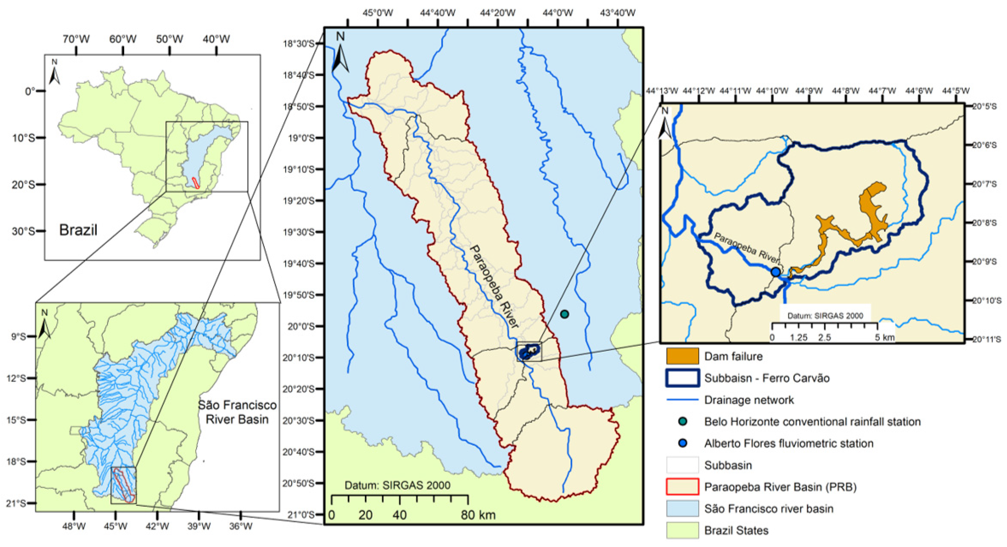
The rupture of the B1 dam occurred in the Córrego do Feijão basin, a tributary drain of the Paraopeba River Basin (PRB). The rupture occurred on 25 January 2019, at an altitude of 100 km from its source, resulting in a 200 km impact at the mouth of the Paraopeba River Basin. The basin is located in the southern region of the State of Minas Gerais and flows into the São Francisco River basin, Brazil (Figure 1). The PRB’s total drainage area is 13,514.94 km², comprising practically 48 municipalities and 2,349,024 inhabitants.

The rupture had a serious impact on regional water security. It was necessary to suspend water collection in a 250 km stretch downstream of the rupture. About 16 cities were affected by the dam failure. The Paraopeba River is the source of drinking water for the Metropolitan Region of Belo Horizonte (RMBH) and other cities. The RMBH has 6 million people, and with the disruption, the supply was compromised by 30% [18,34].

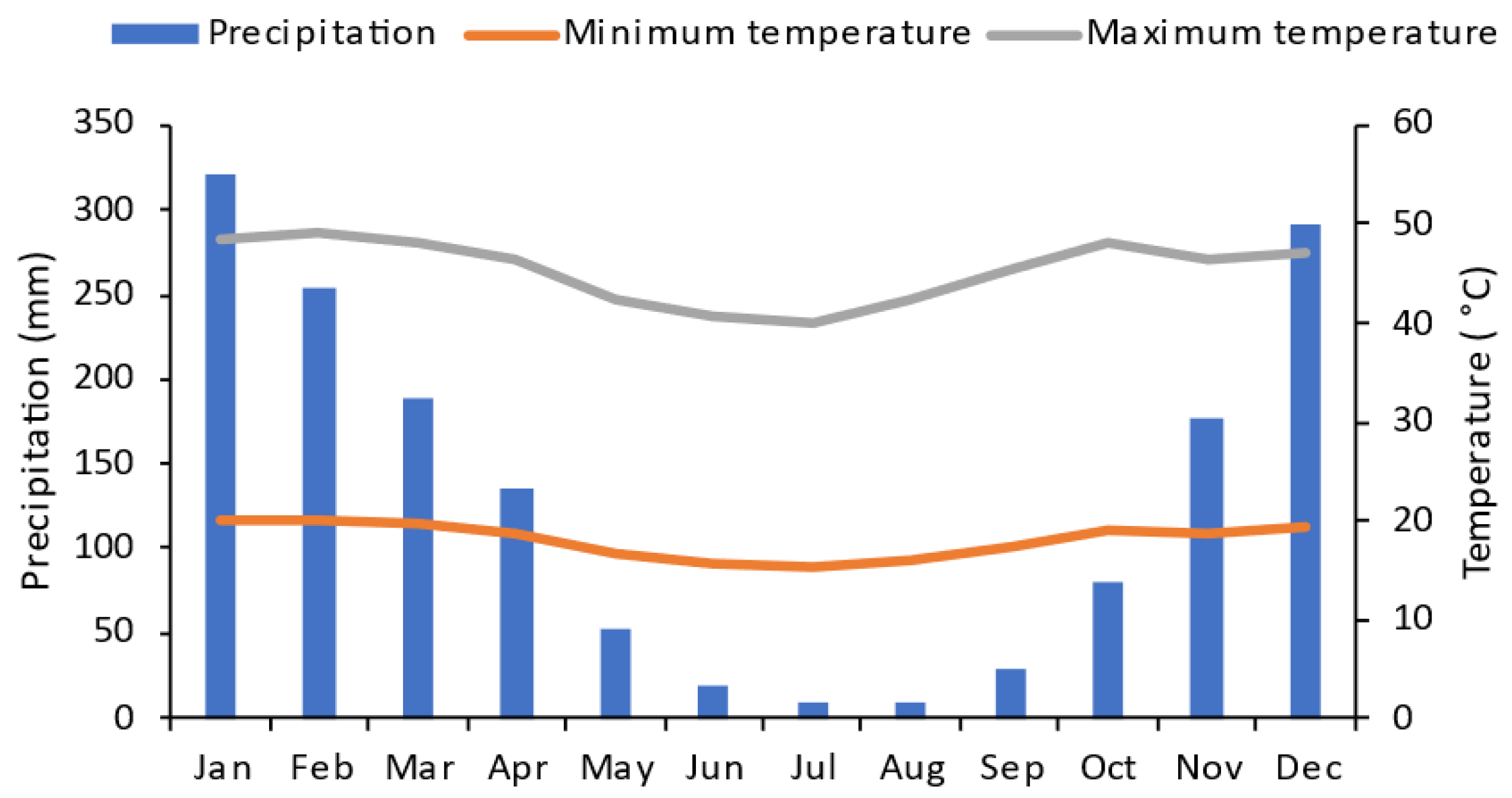
The amount of water in a given watershed depends on the climate and the conditions of land use and cover in the area considered, which directly influence the seasonal behavior of water flows. Due to its greater latitudinal extension around 300 km, the PRB has heterogeneity in its Hot Central Brazil Tropical Climate, in two climate subtypes according to the Köppen classification, Cwa and Cwb, with a humid temperate climate and a dry winter, and with different processes occurring in the summer period, warm in the Cwa and temperate in Cwb [35]. The lowest temperatures (15 °C) occur between the months of June, July, and August, and maximum temperatures are >27 °C from September to March [36]. The average annual precipitation is 2285 mm, with rainy seasons (November to April) and dry seasons (May to October) (Figure 2).

The pluviometric characterization was carried out with an emphasis on the long-term annual variability in the precipitation. The rainfall regime can be considered one of the most important variables for climate study, in addition to significantly influencing the water balance by affecting the surface runoff regime and the recharge of the aquifers. From 2000 to 2021, the highest precipitation generally occurred from December to March, with values varying between 182.5 mm and 320.38 mm in March and January, respectively. The highest rainfall (134 to 320 mm) occurs in the rainy season, while in the dry season, rainfall varies from 8 to 80 mm per month. The monthly minimum and maximum average temperatures were 18 °C and 27.4 °C, respectively (Figure 2). The evapotranspiration of the hydrographic basin varies from 665 to 977 mm according to the Master Plan of the Paraopeba Hydrographic Basin [37].

2.2. Workflow

The model hydrologic response to landscape change scenarios (LULCCs) in river basins with environmental land use conflicts was determined from the SWAT model (Figure 3). Land capability is defined as natural use. It is a powerful resource for land use planning and can be used in the development of public policies [1]. The study sought to evaluate the impact of this land use on the water balance of the hydrographic basin. The protection of more fragile environments with forests is an important tool for soil protection [38]. This method helps to minimize erosion processes in the watershed [2,10] and improve water quality [11].

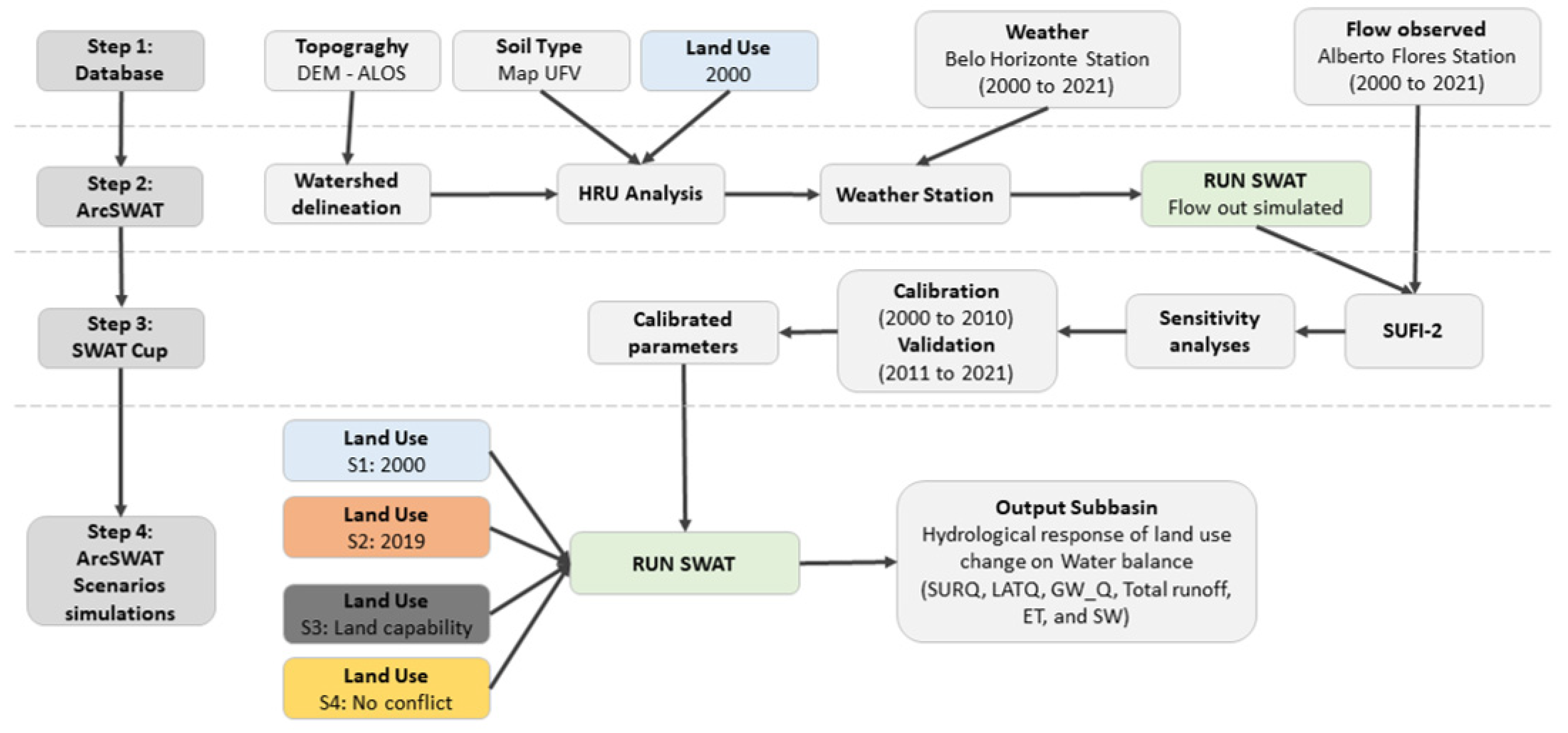
2.3. Data Base

The SWAT model is a continuous basin scale with time intervals and semi-distributed, simulating hydrological processes [39]. The identification of variables in the model has a large-scale approach, and the analysis of each HRU was carried out to identify which parameters indicate, positively or negatively, anthropogenic pressure on the PRB ecosystem. Each HRU was parameterized via SWAT using a series of hydrological response units (HRUs), which will be parts of the HRU that have a unique combination of land use/land management, soil, and topography [29,40].

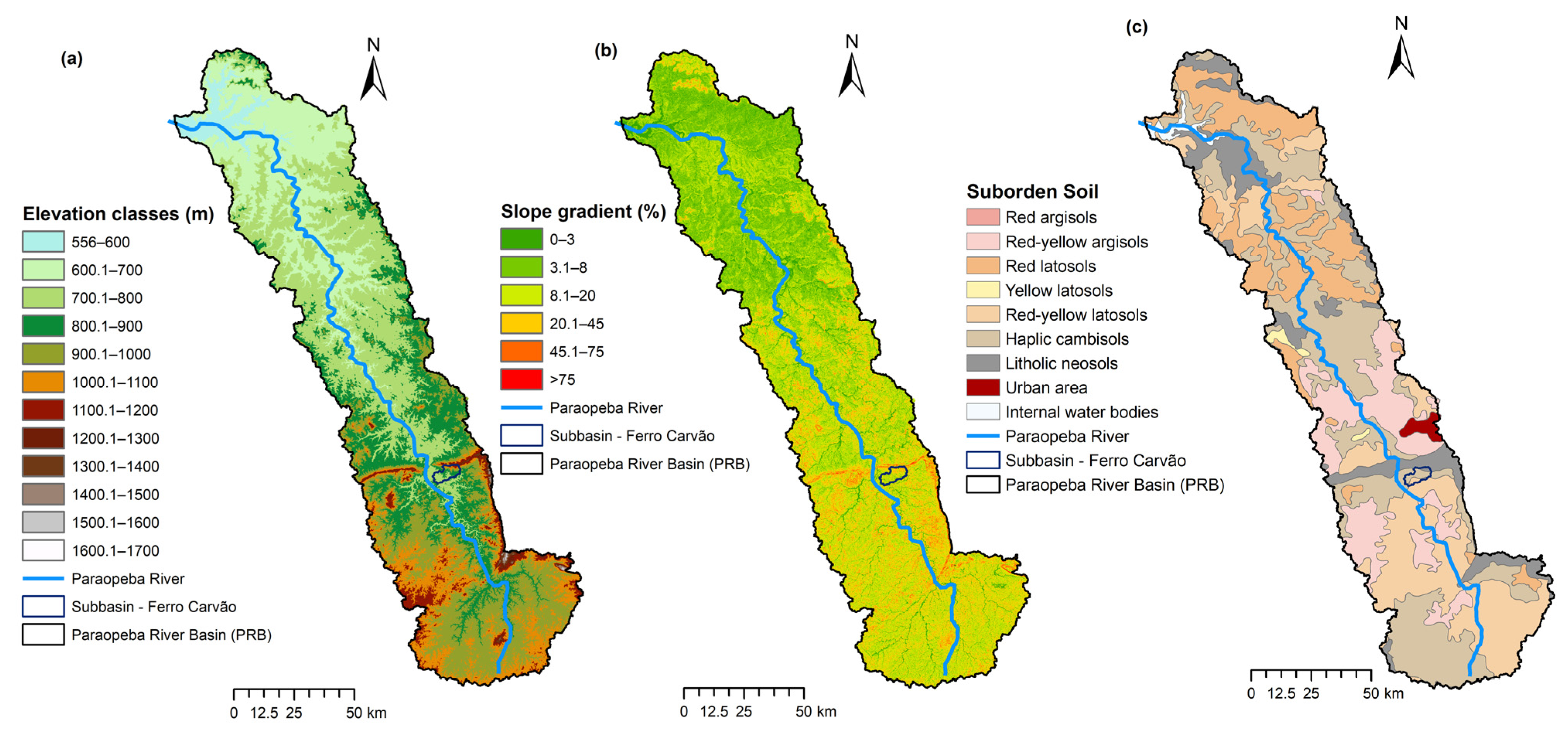
For the composition of the database, we used the raster of the Digital Elevation Model (DEM) of the USGS: US Geological Survey https://search.asf.alaska.edu/# (accessed on 15 April 2022) of spatial resolution 12.5 m, resampled from USGS, and the soil map was obtained from the Soil Map of the State of Minas Gerais https://dps.ufv.br/softwares/ (accessed on 20 May 2022) with a scale of 1:650,000. For the spatial analysis of elevation and slope, the thematic maps of the PRB basin were processed using the elevation data obtained from the terrain DEM (Figure 4a). Thematic maps of elevation, slope, and soil suborder are shown in Figure 4.

For the relief analysis, the slope classes according to the Brazilian Soil Classification System used in the soil mapping units in Brazil [41] were considered: The relief of the PRB ranges from 0 to 100%, with an average slope of 13%, with a standard deviation of 11%. The wavy relief predominates in the area with 38.3%, occupying 5199.0 km² (Figure 4b,

Table 1. Relief classes and percentages of slope in the Paraopeba River Basin [42].

Relief Classes	Slope Gradient (%)	Area (km2)	Area (%)
Flat	0–3	1455.6	10.7
Slightly undulating	3–8	3606.8	26.6
Undulating	8–20	5199.0	38.3
Highly undulating	20–45	3055.4	22.5
Mountainous	45–75	247.3	1.8
Highly mountainous	>75	16.2	0.1
	Total	13,580.4	100.0

Note(s): Source: ALOS image (12.5 × 12.5 m) (https://asf.alaska.edu/, accessed on 16 February 2023).

).

The soil thematic map was processed from the PRB Soil Classes according to the Brazilian Soil Classification System [41]. The most predominant soils in the area are Haplic Cambisol (31%), followed by Red-Yellow Latosol (23%) (Figure 4c,

Table 2. Soil Suborder Classes in the Paraopeba River Basin.

Suborder Soil Classes	Area (km2)	Area (%)
Haplic cambisols	4307.4	31.66
Red-yellow latosols	3143	23.1
Red latosols	2348.6	17.26
Red-yellow argisols	1935.3	14.22
Litholic neosols	1565.7	11.51
Internal water bodies	129.4	0.95
Urban area	107.9	0.79
Yellow latosols	69.3	0.51
Red argisols	0.7	0.01

). Haplic Cambisols, normally found in strong undulating or mountainous relief, without the existence of a superficial to humic horizon, present variable natural fertility with limitations for use due to the accentuated relief, small depth, and the occurrence of stones in the soil mass. The red-yellow latosols have good permeability, are structured and very porous, have good moisture retention, and are very deep soils located in flat or gently undulating relief. Argisols occur in different climatic conditions and source material and are more common in more rugged and dissected reliefs with less smooth surfaces, making them more susceptible to erosion processes [41].

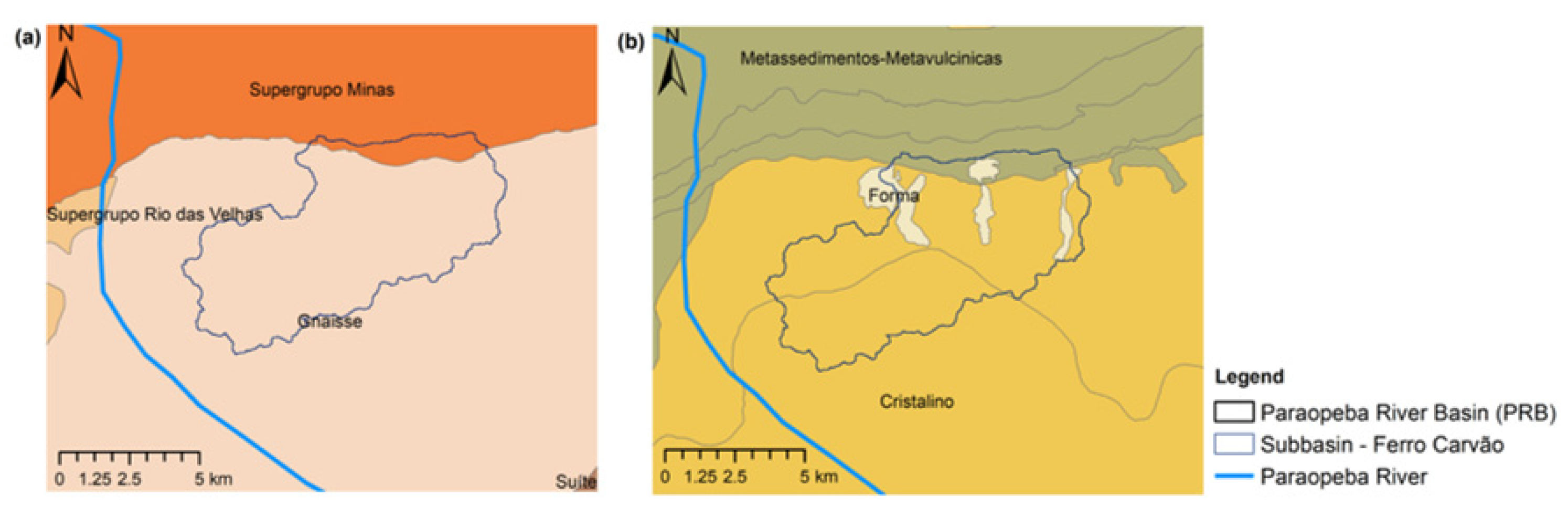
The Paraopeba River Basin has a heterogeneous geology and is formed of about 20 main units (Figure 5a). The predominant geology of the São Francisco Supergroup formation (23.59%) is located downstream of the hydrographic basin. The mining area, where the dam rupture occurred, has a predominance of gneiss formation [43]. The area has a predominance of the Cristalino hydrogeological domain (fissured aquifer) (Figure 5b). In this region, there are shales, phyllites, and quartzites. The type of rock does not have primary porosity; the groundwater occurs in the secondary porosity represented by fractures and fissures that form random reservoirs, discontinuous in small areas, and generally have low flows [44].

2.4. SWAT Model Processing

The model SWAT considers the effects of changes in land use and allows for great flexibility in configuring the proportionality of hydrological phenomena. SWAT made it possible to divide the basin into Hydrological Response Units (HRUs) and is based on the water balance equation [40], in Equation (1):

$$S{W}_t=S{W}_0+{{\displaystyle \sum }}_{i=1}^t(R_{day}-Q_{surf}-E_a-W_{seep}-Q_{gw})$$

(1)

where: SW_t—final water content in the soil (mm); SW₀—soil water content (mm); t—time (days); R_day—precipitation (mm); Q_surf—runoff (mm); E_a—evapotranspiration (mm); W_seep—water percolation from the simulated layer to the bottom (mm); and Q_gw—lateral flow (mm).

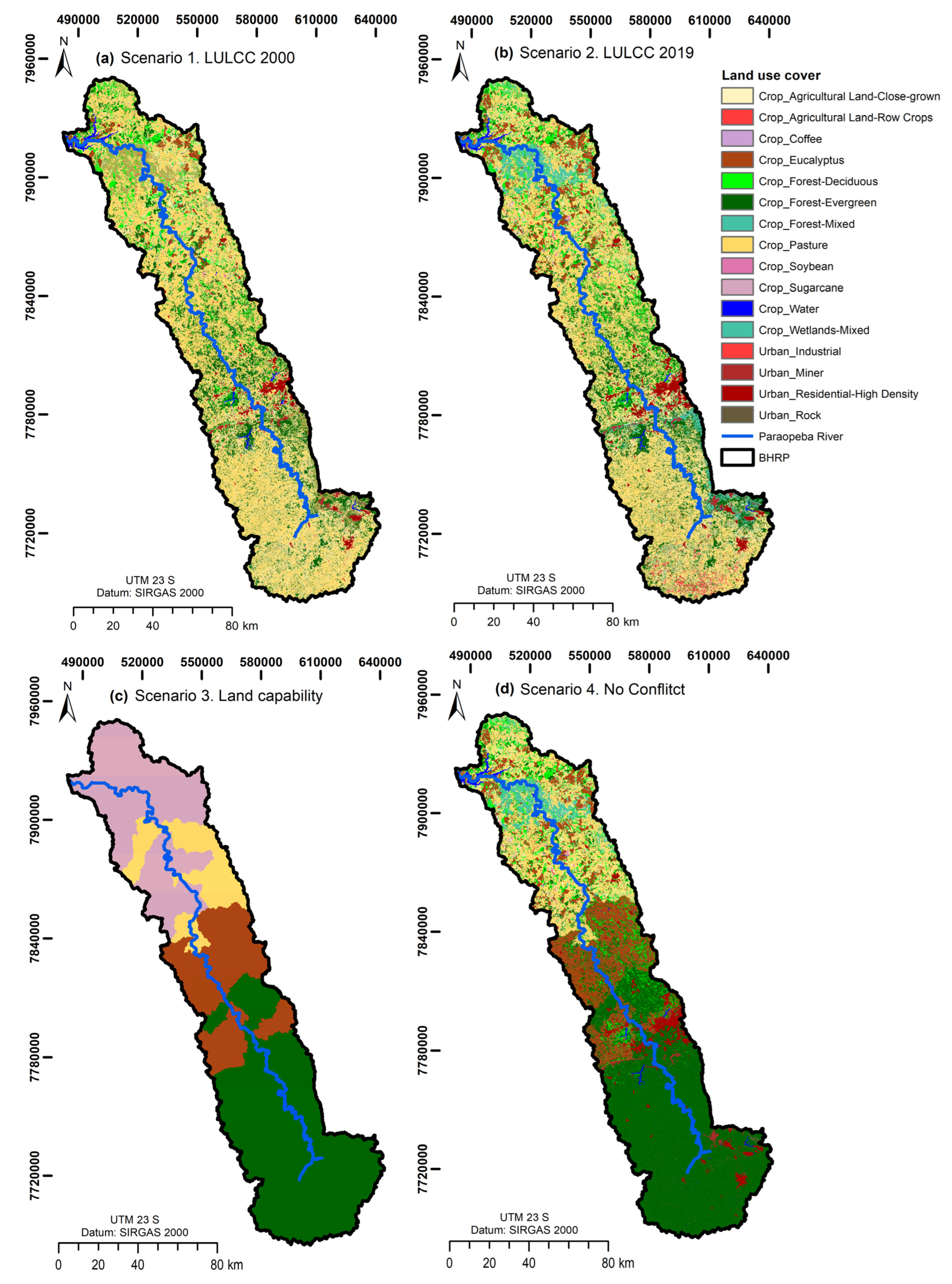
For the initial processing of the model, several periods of the climate database were tested. At the beginning of processing, the land cover was selected for the year 2000—LULCC 2000 (S1). All land use parameters were obtained from the SWAT database. The parameters of native vegetation, eucalyptus, pasture, and agriculture were modified as maximum leaf area index (BLAI), canopy stomatal conductance (GSi), and Manning’s “n” for surface (OV_N) from the SWAT model database to better represent tropical conditions according to Martins (2021). The soil suborder parameters in the SWAT model were characterized according to studies by Baldissera [32], Freire [45], Lima [46], and Moreira [47]. The input climatic parameters for the SWAT model, such as precipitation, relative humidity, temperature, solar radiation, and wind speed, were obtained from daily historical series of Belo Horizonte conventional rainfall station, from 1 January 1997 to 31 December 2021, obtained from the National Institute of Meteorology (INMET) of the Ministry of Agriculture, Livestock, and Supply (https://bdmep.inmet.gov.br/ (accessed on 15 August 2022)) in Brazil (Figure 1). The station was chosen due to its proximity to the PRB zone structural failure and its performance in modeling the PRB water balance. The daily values were processed in the WGN Parameters Estimation Tool software, and the solar insolation data (hour) were converted to solar radiation (MJ/m²) according to Salati [48]. The Penman–Monteith equation was used to compute the evapotranspiration in SWAT.

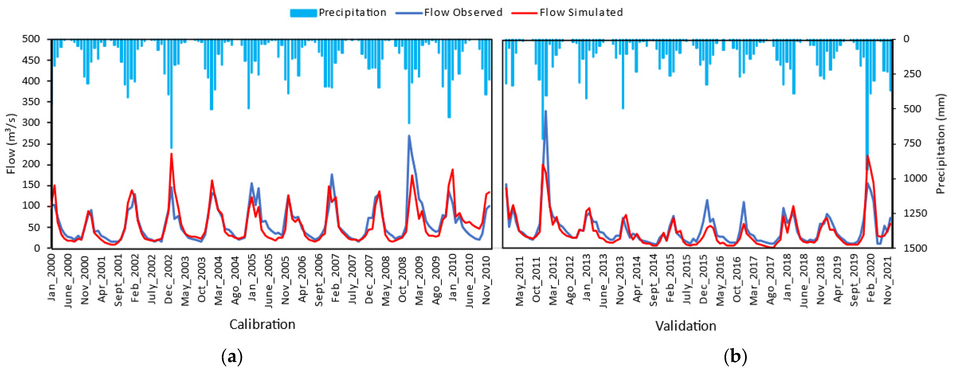
The hydrological calibration of the PRB was carried out using the database obtained from the Alberto Flores fluviometric station (Figure 1), considering that this area is located as close as possible to the outflow of the zone of structural failure. Historical flow data were obtained from fluviometric stations of the Sistema Nacional de Informação de Recursos Hídricos (SNIRH) and the Agência Nacional de Águas e Saneamento Básico (ANA) (https://www.snirh.gov.br/hidroweb/serieshistoricas (accessed on 10 June 2022)). For the calibration, the historical series from 1 January 2000 to 31 December 2010 and the validation from 1 January 2011 to 31 December 2021 were used.

The calibration method employs inverse modeling (IM) and indicates physical system inferences based on the flow variable [49,50]. Measurements are subject to uncertainties, and inferences are generally statistical in nature. Physical systems use continuous equations, so the inverse hydrological problem is not uniquely solvable. The objective of inverse modeling was to characterize a set of models by assigning uncertainty distributions to the parameters that fit the data and satisfied the assumptions.

The model was calibrated in SWAT-CUP (SWAT Calibration Uncertainty Program), using the Sequential Uncertainty Fitting (SUFI-2) method as an optimization program [51]. SUFI-2 is a method like the inverse Bayesian, which combines objective function optimization and uncertainty analysis and allows for dealing with a large number of parameters in the calibration of a numerical model. Calibration adjustment used 95 Percent Prediction Uncertainty (95PPU), calculated at the 2.5% and 97.5% levels of the cumulative distribution of an output variable generated by the propagation of parameter uncertainties using Latin hypercube sampling, disallowing 5% of the very bad simulations.

To quantify the fit between the simulation result, expressed as 95PPU, and the observation, expressed as a single signal, two statistics must be adhered to: P factor and R factor [50,51]. The P factor is the percentage of observed data involved in the modeling result. The R factor is the thickness of the 95PPU envelope. The value of the P factor varies between 0 and 100%, while that of the R factor varies between 0 and infinity. A P factor of 1 and R factor of 0 make up a simulation that exactly matches the measured data. In the modeling process, the aim was to find the highest P factor (above 0.7) with the lowest R factor (less than 1.2) for flow.

Additional better fit was quantified by R², Nash–Sutcliff (NS), and PBIAS between observations and the most appropriate final simulation. It is emphasized that the best simulation occurs when the range of the final parameters is within the ideal values of these coefficients. There are no ideal numbers for the response of the R² or NS coefficients; the higher the value, the better the simulation statistics.

The performance of the model was analyzed using the Nash and Sutcliffe [52] coefficient (NS) and the percentage of trends (PBIAS), Equation (2):

$$NS=1-\frac{{{\displaystyle \sum }}_{i=1}^n{\left(Q_{obs}-Q_s\right)}^2}{{{\displaystyle \sum }}_{i=1}^n{\left(Q_{obs}-\overline{Q}\right)}^2}$$

(2)

where $Q_{obs}$ is the observation for the constituent being evaluated, $Q_s$ is the simulated value for the constituent being evaluated, $\overline{Q}$ is the mean of the observed data for the constituent being evaluated, and n is the total number of observations (Equation (2)). The NS can vary from infinite negative to 1, and the closer to 1, the better the calibration is evaluated.

The percentage of trends (PBIAS) is calculated by Equation (3), and the closer it is to zero, the better the result.

$$PBIAS=\frac{{{\displaystyle \sum }}_{i=1}^n\left(Q_{obs}-Q_s\right)}{{{\displaystyle \sum }}_{i=1}^n{Q}_{obs}}$$

(3)

where Q is a variable (e.g., flow; flow) and m and s represent measured and simulated, respectively. PBIAS measures the average tendency of simulated data to be larger or smaller than observations. The optimal value is zero, where low-magnitude values indicate better simulations. Positive values indicate model underestimation, and negative values indicate model overestimation [53]. Calibration and validation results were classified according to Moriasi [54].

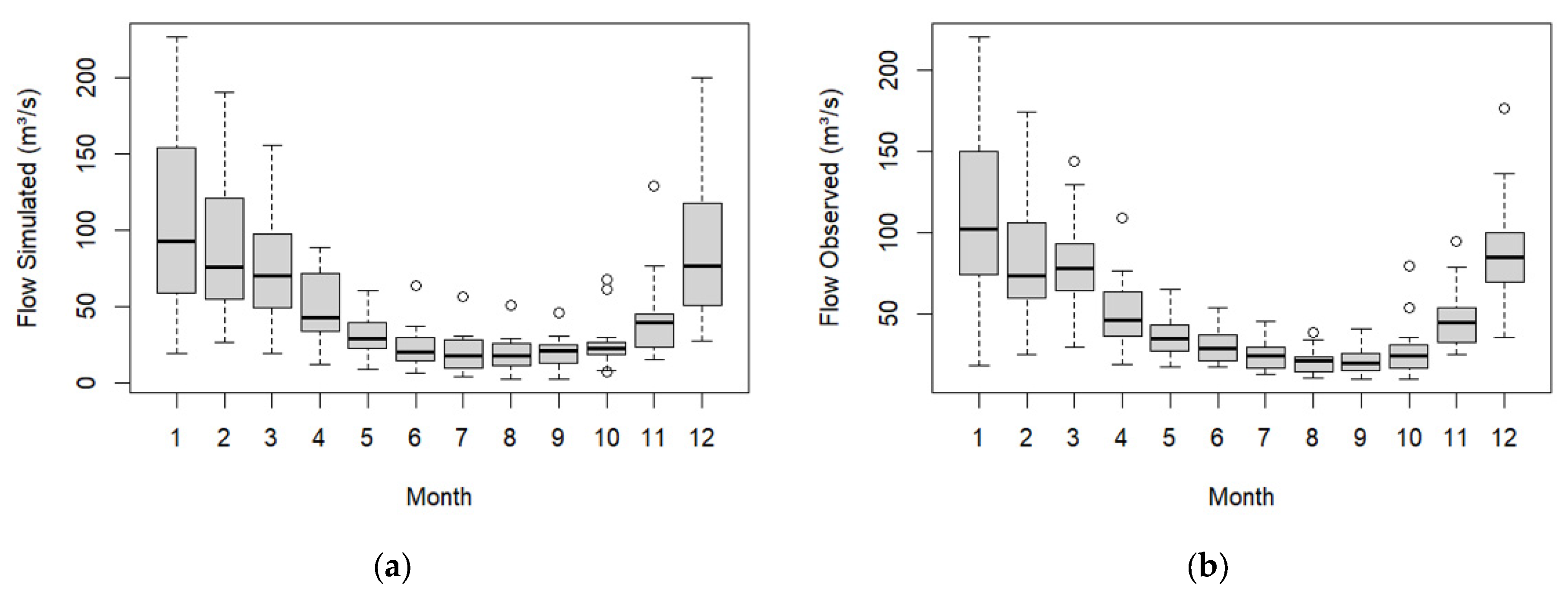
The SWAT model can safely monitor the discharge of the Paraopeba River Basin. The parameters of the SWAT model for monitoring the risk of flooding and the risk of water scarcity are based on the simulated water volume (flow) for the Paraopeba River.

The model can be used to expand the spatial and temporal monitoring capacity at a lower operational cost. Simulated data can be added to visualization panels for year-round monitoring at any point in the basin. The analysis was carried out based on the range of quartiles for the dry and rainy months of the flow data simulated by the model. The flood risk occurs when the flow in the watershed exceeds the 3rd quartile. When this occurs, the volume of water rises above the river channel and overflow occurs, causing flooding. The risk of water scarcity occurs when the water flow is below the 1st quartile. Low water volume can pose a danger to water availability and increase the risk of increased concentrations of pollutants in the water. The indicators can be used in a dashboard by entities to monitor the Paraopeba watershed.

2.5. Land Use Conflict

For the diagnosis of land capability and the land use conflict in the scenarios, the PRB needed to be compartmentalized into hydrological response units (HRUs). The compartmentation of the PRB into physiographic units was carried out from 33 monitoring points [36,55] with the aim of understanding the natural open systems that drain surface water into the thalweg of the Paraopeba River. Each HRU was delineated from the points of higher elevations forming the lines of the topographic dividers and the lines with the points of lower elevations constituting the drainage networks [13].

The cartographic base of land use was made available by the Annual Land Use and Coverage Mapping Project (https://mapbiomas.org/ (accessed on 30 April 2022)), in the 2019 image taking, reclassified for land uses of Residential/Industrial, Agriculture, Pasture, and Forestry. The PRB has a predominance of pasture (63%), followed by forest (27%).

The environmental indicator, Ruggedness Number (RN), was introduced by Strahler [56]. This indicator is used as a morphometric parameter of a watershed to understand the relationship between the total length of the drainage network over a given area (Drainage density (Dd) and Slope (S) (Dd × S)). Therefore, it was possible to compare river basins with this indicator to understand hydrological dynamism [3,4,38]. The model used in the present study defined the land use capability from four classes determined by the Natural Breaks method (Jenks). RN classes were reclassified with capability land use, from smallest to largest, as: agriculture, pasture, forestry, and native forest.

The Land Use Conflict indicator was introduced by Mello Filho and Rocha [57] and later modified by Valle Junior [58] and Valle Junior [59]. According to these authors, the Land Use Conflict (C) classes occur when the land capability (UP) deviates from actual use (UA) (Equation (1)).

Land Use Conflict (C) = Weight UP_i − Weight UA_j, com 1 ≤ i ≤ n e 1 ≤ j ≤ n

(4)

For the analysis of deviations between the UP and the UA, the respective identification codes were used. The class actual use (UA) and land capability (UP) were assigned weights, agriculture weight 1, pasture weight 2, forestry/eucalyptus weight 3, and natural forest weight 4, according to Valle Junior [4,58]. The mathematical calculation generates negative and zero results, which are classified as regions without Land Use Conflict, and positive results (1, 2, 3) are the levels of conflict. 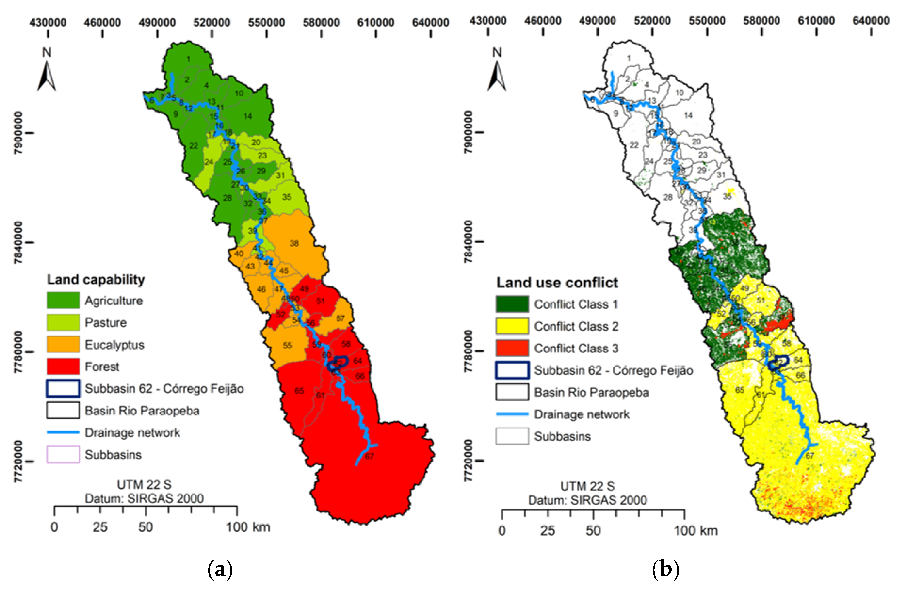The Conflict class 1 area can be represented by regions where the deviation of an immediately higher class occurs while conflict Class 2 or Class 3 with greater deviations, according to Valle Junior [4] (Figure 6).

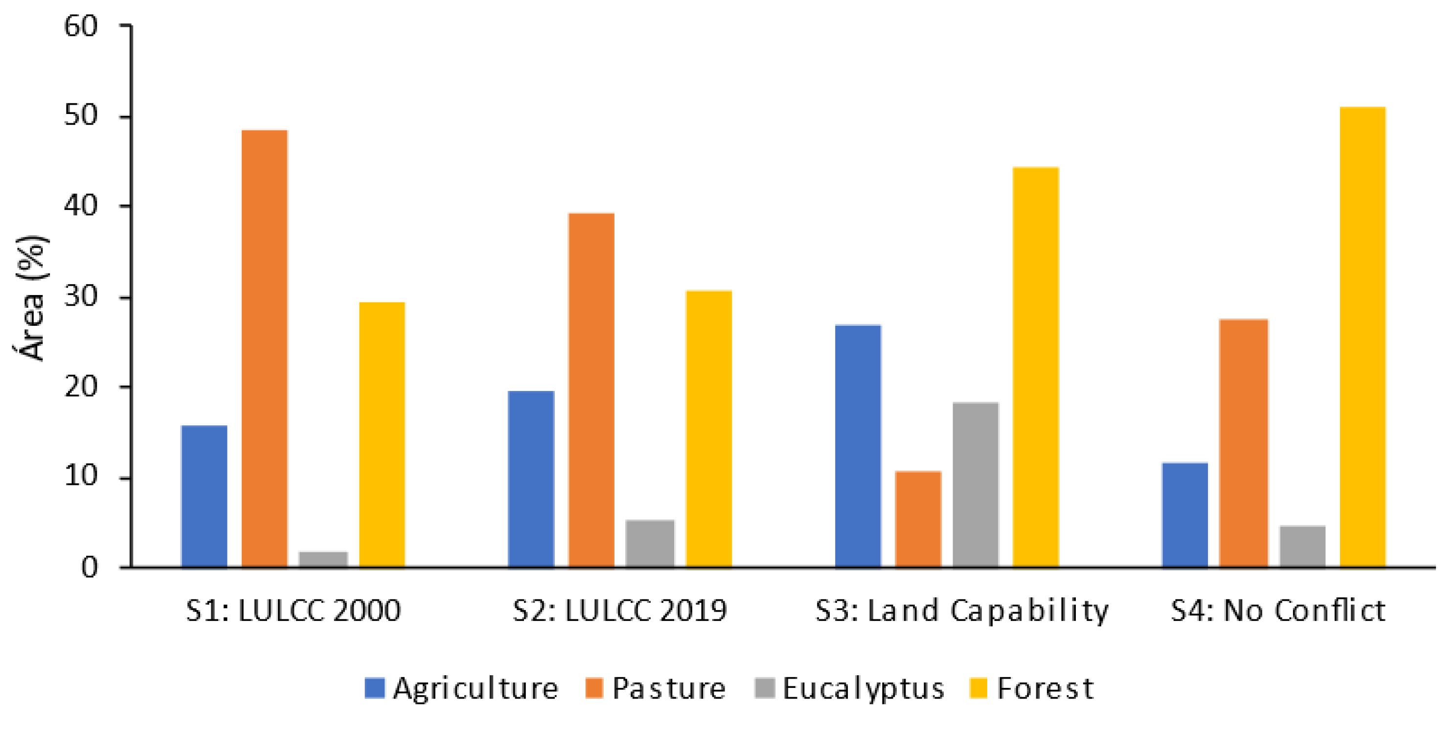
The land capability of the Paraopeba River Basin (PRB) varies longitudinally (Figure 6a). The most sloping areas with higher drainage density and forest land capability (44.3%) are located upstream from the PRB, and downstream are the flatter areas with lower drainage density (25.8%). In the central part of the basin, the intermediate pasture and forestry capabilities are located, with 10.5% and 18.3%, respectively.

At PRB, land use conflict occupies almost half of its area (43%), with conflict class 2 being the most common (29%) (Figure 6b). Conflict class 1 occurs in relief environments, ranging from undulating to heavily undulating, where intensive plant and animal production systems occur. Intensive agriculture presents soil preparation management, farming, and harvesting with an intense use of agricultural mechanization. Therefore, in order to avoid a negative impact on the environment, it is recommended in areas with greater slopes, better management practices, and soil and water conservation. As seen in Figure 6, the area that presents the greatest conflict (Class 2) is the southern region (upstream of the basin). Class 2 conflict was also predominant in 41% subbasin 62, affected by the dam failure due to the high coefficient of roughness and natural ability to the natural vegetation of the forest.

2.6. Land Use Land Cover Scenarios

For the analysis of the hydrological performance of the Paraopeba River Basin (PRB), three scenarios were carried out after the calibrated basin (

Table 3. Scenario of LULCC in the Paraopeba River Basin.

Scenarios	Name	Description
Scenario 1	LULCC 2000	Land cover for the year 2000.
Scenario 2	LULCC 2019	Land cover for the year 2019
Scenario 3	Land Capability	Land capability according to the RN coefficient.
Scenario 4	No Conflict	Land cover for the year 2019 without land use conflict. Areas of conflicting use were replaced by their land capability.

and Figure 7).

The scenarios were built to verify the impact of land use on the hydrological components of the Paraopeba River Basin. The scenarios allow for estimating the components of the water cycle at any location in the calibrated watershed, determining the best alternatives for political land use management [25,26]. The response to land use change was analyzed according to parameters: precipitation, evaporation and transpiration, PET, revap from shallow aquifer, surface runoff, lateral flow, and return flow. Potential evapotranspiration (PET) is the process by which water is lost to the atmosphere by water transfer through soil evaporation and plant transpiration.

The response to land use change was analyzed according to the following parameters of the hydrological model: Surface runoff (SURQ), Lateral flow (LATQ), Groundwater (GW_Q), Total runoff, Actual evapotranspiration (ET), and Soil water content (SW) (

Table 4. Parameters used to evaluate the effect of land use change on the Water Balance of the Paraopeba River Basin.

Parameters	Description
SURQ	Surface runoff contribution to streamflow during time step (mm).
LATQ	Lateral flow contribution to streamflow during time step (mm)
GW_Q	Groundwater contribution to streamflow (mm). Water from the shallow aquifer that returns to the reach during the time step.
Total runnoff	Total surface runoff (mm)
ET	Actual evapotranspiration from the HRU during the time step (mm).
SW	Soil water content (mm). Amount of water in the soil profile at the end of the time period.

).

3. Results

3.1. Calibration and Validation of the Hydrological Model

The values of the hydrological parameters adjusted above obtained acceptable values in the adjustment indicators for calibration and validation with Alberto Flores fluviometric station and LULCC 2000 (S1). Thus, 14 parameters were used in the calibration of the SWAT model for the Paraopeba River Basin. The model was optimized using the sensitivity analysis tool, and the best three parameters that had the most significant influence on the calibration (p ≤ 0.05) were RCHRG_DP, SLSUBBSN, and GWQMN (

Table 5. Parameters used in the flow calibration procedure between 2000 and 2010 in the Paraopeba River Basin. In the method legend, R is relative and V is the replacement value. (*) represents statistically significant parameters (p ≤ 0.05).

Parameter	Description	Units	Minimum	Maximum	Fitted Value
R__CN2.mgt *	Curve number for moisture condition II		−0.10	0.10	−0.167172
V__ALPHA_BF.gw *	Baseflow alpha factor	days	0	1.00	0.853566
V__GW_DELAY.gw	Groundwater delay	days	0	500.00	500
V__GWQMN.gw *	Flow threshold depth of water in shallow aquifer		0	5000.00	3277.24707
V__REVAPMN.gw *	Threshold depth of water in the shallow aquifer for “revap” to occur	mm	0	500.00	73.709579
V__GW_REVAP.gw *	Groundwater “revap” coefficient.		0.02	0.20	0.034165
V__RCHRG_DP.gw *	Deep aquifer percolation fraction.		0	1.00	0.395725
V__CH_K2.rte	Effective hydraulic conductivity in main channel alluvium.		−0.01	500.00	150.156586
V__ESCO.hru *	Soil evaporation compensation factor.		0	1.00	0.554175
V__EPCO.hru *	Plant uptake compensation factor.		0	1.00	0.596485
V__SLSUBBSN.hru *	Average slope length.		10.00	150.00	51.052189
R__SOL_AWC(..).sol	Available water capacity of the soil layer.		0.00	1.00	0
R__SOL_K(..).sol *	Saturated hydraulic conductivity.		0.00	2000.00	1.235092
V__SURLAG.bsn	Surface runoff lag time.		0.05	24.00	24

).

The model adjustment ended with the p-value and r-factor coefficients obtaining acceptable values in calibration and validation (

Table 6. Goodness-of-fit indicators for monthly calibration between 2000 and 2010 and the validation of streamflow between 2011 and 2021 in the Paraopeba River Basin. Calibration and validation results were classified according to Abbaspour [50,51] and Moriasi [54].

Measures	Values	Acceptable Ranges
Calibration
P-factor	0.83	>0.7 good
R-factor	0.83	<1.2 good
NSE (Nash–Sutcliffe Efficiency)	0.66	0.65–0.75 good
R2 (Coefficient of determination)	0.69	0.65–0.75 good
PBIAS	5.2	±10 very good
RSR (Standardized RMSE)	0.59	0.5–0.6 good
Validation
P-factor	0.8	>0.7 good
R-factor	0.78	<1.2 good
NSE (Nash–Sutcliffe Efficiency)	0.74	0.65–0.75 good
R2 (Coefficient of determination)	0.77	0.65–0.75 good
PBIAS	13.5	±10–±15 good
RSR (Standardized RMSE)	0.51	0.5–0.6 good

). The p-value remained above 0.7 in calibration and validation, at 0.83 and 0.8, respectively [50,51]. To assess the additional quality of the model statistical adjustment, the correlation coefficients were observed (Table 6). The goodness statistical adjustment indicators for flow rate showed good and very good performance of the model, both in calibration and validation. Analysis of NSE values was 0.66 (good) and 0.74 (good) for both calibration and validation, respectively. R² showed good and very good model performance with values of 0.69 and 0.77 for calibration and validation, respectively. In the calibration, the model presents a slight overestimation (5.2%) of the simulated flow, and in the validation, an overestimation (13.5%). RSR analysis shows values of 0.59 (very good) and 0.51 (good) for calibration and validation, respectively.

The analysis of the distribution of the simulated/observed flow in relation to the precipitation demonstrates that the data follow a trend, indicating an adjustment of the model in relation to the observed data (Figure 8).

According to the precipitation data, the volume of water influenced by the seasons is 233 mm on rainy days and 31 mm on dry days. The water availability in the basin system corresponds to the average flow of rainy 76 m³/s and dry 31 m³/s.

In the dataset, seasonal validation is observed where there is a rainy period and a dry period. In the rainy season, the highest values of 935 mm occur, which indicates the presence of extreme events of flow (328 m³/s). The hydrograph expresses the superimposition of flow values (Figure 8).

The simulated and observed peak flow indicates that the model has low performance in the dynamics of extreme events. The PBIAS and RMSE are significantly reduced in periods of no extreme events. The results obtained were satisfactory and met the pre-established objectives of presenting the statistically adequate performance of the model.

3.2. Water Balance of the Paraopeba River Basin

The water balance of the Paraopeba River Basin is shown in

Table 7. Water balance simulated by SWAT between 2000 and 2021 with LULCC 2000 (S1) in the Paraopeba River Basin.

Water Balance Parameters	S1: LULCC 2000
Precipitation	1548
Evaporation and Transpiration	850
PET	1149.9
Revap from shallow aquifer	39.33
Surface Runoff	112.86
Lateral Flow	228.54
Return Flow	84.32
Percolation to shallow aquifer	349.44
Recharge to deep aquifer	138.27
Total Flow	425.72

. The average rainfall for the study period was 1548 mm. The evapotranspiration and simulated transpiration of 850 mm can be validated with the value found in the Master Plan of the Paraopeba Watershed, which varies from 665 to 977 mm [37]. The evapotranspiration value was selected to indicate the simultaneous process of transferring water to the atmosphere of the PRB from the evaporation (E) and transpiration (T) processes. This value indicates the amount of water used by the main land use in each growing hydrological region (HRU), which completely covers the soil and has no water restrictions, which is equivalent to reference evapotranspiration (ET0).

The variables were influenced by LULCC, soil, and slope on a basin scale, as well as by climate. To determine the amount of water available as flow in the PRB, other variables need to be analyzed. The model determined the water balance through an indirect estimate involving the values of the processes that were calibrated and validated. The evapotranspiration (1149.9 mm) and rainfall (1548 mm) were obtained by taking the average of the annual values from the historical series. Evapotranspiration in a watershed is the component of the water cycle that has the greatest uncertainty. In relation to the order of magnitude, the precipitation and the surface runoff (112.86 mm) are also important, since in many regions, this variable represents a greater proportion of precipitation than the deflection (Table 7).

The water at the surface of the basin is concentrated in a lateral flow of 228.54 mm, followed by surface runoff of 112.86 mm and return flow of 84.32 mm. In the groundwater, the highest proportion is present in the percolation of the shallow aquifer (349.44 mm), and the lowest proportion goes to the recharge of the deep aquifer (138.27 mm).

Water balance rates for land use in 2000 are expressed in mm and are an annual average between 2000 and 2021 in the Paraopeba River Basin (

Table 8. Water balance ratios simulated by SWAT between 2000 and 2021 with current land use of the Paraopeba River Basin.

Water Balance Ratios	S1: LULCC 2000
Surface runoff/Total Flow	0.27
Lateral flow/Total Flow	0.54
Groundwater Flow/Total Flow	0.20
Streamflow/Precipitation	0.28
Percolation/Precipitation	0.23
Deep recharge/Precipitation	0.09
Evapotranspiration/Precipitation	0.55

). The largest amount of water that reaches the river comes from the lateral flow (54%), with the remainder coming from surface runoff and groundwater flow at 27% and 20%, respectively. In the basin, the streamflow corresponds to 28% of the precipitated water. About 55% of the precipitated water from the basin returns to the atmosphere through evapotranspiration, and only 9% of the precipitation goes to deep recharge.

3.3. Hydrological Model for Flood Risk and Risk of Water Shortage

Figure 9a shows that the SWAT model was efficient in representing the monthly variability in the flow at the fluviometric station Alberto Flores and that conditions can be accompanied and monitored using this model from these other points in the Paraopeba River Basin. The observed flow showed greater amplitude due to the existence of an extreme flow event with an outline of 328.37 m³/s in January. The watershed regions that already face shortages of water resources are among the most affected by the drop in groundwater recharges. Figure 9b shows that the area might face more frequent flows due to the expected change in climate variability and the occurrence of extreme climate events, so the government must develop new hydrological plans.

Due to the need to monitor water resources, simulated flow data were used to compose a risk analysis method. The method used quartile flow to define zones of risk of flooding and risk of water scarcity (

Table 9. Flood risk and water scarcity risk by month flow (m³/s) for the Alberto Flores fluviometric station determined from the monthly variation flow simulated.

Risk Indicator	Minimum	Q1.25%	Median	Q3.75%	Maximum
Flood risk	11.9–27.3	23.4–69.3	39.3–96.4	44.9–120.5	88.6–226.5
November	15.6	23.4	39.3	44.9	129.2
December	27.3	57.9	78.6	107.4	200.1
January	19.1	69.3	96.4	162.8	226.5
February	26.5	54.4	75.9	120.5	190.2
March	18.9	49.3	69.7	97.2	155.4
April	11.9	34	42.4	70.3	88.6
Water scarcity risk	2.3–9.0	10.0–22.7	17.5–29.3	24.8–39.0	46.0–67.8
May	9	22.7	29.3	39	60.2
June	6.2	15	20.1	30	63.9
July	3.8	10	17.5	27.7	56.5
August	2.6	10.9	17.6	25.8	50.3
September	2.3	12.6	21.2	24.8	46
October	7.5	18.8	22.7	26.2	67.8

). The red hue presents the highest risk intervals and the green the lowest risks for each month.

The greatest flood risk may occur between Q3.75 and maximum flows. The overflow of water that submerges land occurs mainly in December, January, and February (>190 m³/s). The flood warnings can be seen in Table 9, which shows the values for the risk of flooding (226.5 m³/s). The volume of water flowing along the river impacts is expected to continue until at least mid-February; thus, it will be necessary to pay attention to those points of risk.

In the months of low precipitation (drought), monitoring is carried out to diagnose the risk of water shortages. The greatest risks of drought occur at minimum and Q1.25%. The most worrying months are July, August, and September. The urban supply points downstream of the Brumadinho dam rupture should be activated in these months to assess the potability of the water intended for public supply. The decrease in the volume of water in the river increases the probability that contaminants from the waste are in greater concentration in the water of the Paraopeba River. According to Table 9, the lowest discharge values occur between the months of July and September, where the minimum can be below 3.8 m³/s. The range from 2.3 to 22.7 m³/s is the water shortage risk value for the Alberto Flores fluviometric station.

According to the results, water problems and flooding may occur for flows higher than 44.9–120.5 m³/s, and flows lower than 10.0–22.7 m³/s will suffer water shortages. Furthermore, shifts in precipitation patterns will bring changes in aquifer recharge.

3.4. Response of the Model SWAT to Different Land Use Scenarios

The analysis of hydrological impacts of land use conflicts was evaluated by the SWAT model. Scenarios of no conflict and land capability showed important instruments for territorial management. In these scenarios, the decrease in surface runoff helps to reduce the flow of tailings to the Paraopeba river channel.

Table 10. Comparison of the Water Balance of the LULCC 2019 with Scenario 3: Land Capability and Scenario 4: No Conflict.

Water Balance Parameters	Land Use 2019	Land Capability			No Conflict
	Total	Total	Δ	Δ%	Total	Δ	Δ%
Evaporation and Transpiration	837.2	849.5	12	1%	863.1	25.9	3%
PET	1149.8	1149.8	0	0%	1149.8	0	0%
Revap from shallow aquifer	39.12	39.32	0	1%	39.32	0.2	1%
Surface Runoff	97.93	83.55	−14	−15%	77.98	−19.95	−20%
Lateral Flow	388.65	245.05	−144	−37%	244.82	−143.83	−37%
Return Flow	23.99	92.46	68	285%	87.67	63.68	265%
Total Flow	510.57	421.06	−90	−18%	410.47	−100.1	−20%
Percolation to shallow aquifer	219.76	361.22	141	64%	353.76	134	61%
Recharge to deep aquifer	86.96	142.94	56	64%	139.98	53.02	61%

summarizes the average annual values of current land use and the average annual change and percentage change values of both scenarios for the same components analyzed in Figure 10. In the last few years, the basin showed land use dominated by pasture, which was in disagreement with its capability use. The Land No Conflict of 20.5% increase in the FRSE area led to a decrease of 19.95 mm (20%) in surface runoff, 100.1 mm (20%) in total flow, and 143.83 mm (37%) in lateral flow, and an increase of 63.68 mm (256%) in return flow, 134 mm (61%) in percolation to shallow aquifer, 53.02 mm (61%) in recharge to deep aquifer, and 25.9 mm (3%) in evapotranspiration (Table 10).

The results in Figure 11 show that all parameters showed monthly variations that correspond to seasonal variations in precipitation during the rainy season (November to March) and the dry season (April to October). Scenario 2, corresponding to land cover in 2000, is highlighted. It can be seen that the actual change in land use cover over the past 19 years increased the lateral flow (LATQ) (Figure 11b) and considerably reduced the water stored in the shallow aquifer (GWQ) (Figure 11c), thus increasing the total runoff (Figure 11d). The decrease in the capacity of the basin to retain water in the rainy season can affect the water supply in the dry season.

The results show that all components in the water balance showed monthly variations, with generally higher values between December and May, which correspond to the rainy season (Summer and Autumn), and lower values between June and November, which correspond to the dry season (Winter and Spring) (Figure 11). The monthly SURQ of the forest scenario was the component that showed the greatest differences under land cover scenarios, with most changes occurring during the rainy season from December to May. Less notable changes were observed in other water balance components in the forest scenario and all components in the grassland scenario.

Scenarios 2 and 3 had little difference in parameters. The highest values of GWQ and SW in the watershed on the use capacity show an increase in soil water retention. This scenario is important to reduce the risk of water scarcity during dry periods. Another positive aspect is that PRB land cover does not need to be fully converted for capability land use to achieve this performance. The reversion of areas with land use conflict to capability land use can generate significant gains in water storage and a decrease in surface runoff (Figure 12).

When the average annual values of land cover for 2000 and of 2019 are compared (19 years), they show that changes in land use influenced the hydrological behavior of the Paraopeba River Basin (Figure 12 and

Table 11. Land Use Change from 2000 to 2019.

Hydrological Parameters	S1: LULCC 2000	S2: LULCC 2019	Δ	Δ%
SURQ	115	98	−17	−14%
LATQ	228	389	160	70%
GWQ	93	24	−69	−74%
Total Runoff	436	511	75	17%
SW	304	287	−17	−6%
ET	854	837	−17	−2%

). A 70% increase in lateral runoff (LATQ) and a 74% decrease in shallow aquifer groundwater (GWQ) were observed. Lateral runoff can expand the scope of the original contamination and enhance the lateral migration of heavy metals into the soil [21]. The tailings deposited in the basin, mainly iron and manganese, spread through the water and negatively contribute to the quality of the river [14]. In this way, minimizing surface runoff in these regions can help stabilize these contaminants in the rupture area. The forest areas in the landscape reduce the speed of surface runoff and make it difficult for the tailings to reach the river thalweg [60].

The scenarios of Land Capability and No Conflict may be used to reduce heavy metal contamination along the watershed. As we can see in Figure 12, these scenarios make it possible to reduce lateral runoff (LAT) and increase water infiltration into the soil (GWQ). Simply returning to the land capability uses in the regions of conflict of use, the basin returns to the lateral flow and groundwater levels of 19 years ago.

Table 12. Comparison of the Water Balance of the S2: LULCC 2019 with S3: Land Capability and S4: No Conflict.

Hydrological Parameters	S2: LULCC 2019	S3: Land Capability			S4: No Conflict
	Total	Total	Δ	Δ%	Total	Δ	Δ%
SURQ	98	84	−14	−15%	78	−20	−20%
LATQ	389	245	−144	−37%	245	−144	−37%
GWQ	24	92	68	285%	88	64	265%
Total Runoff	511	421	−90	−18%	410	−100	−20%
SW	287	297	9	3%	296	8	3%
ET	837	849	12	1%	863	26	3%

summarizes the average annual coverage values for 2019, comparing the annual average values and the percentage change with both scenarios. The absence of land use conflict is capable of reducing the SURQ by 20% and the LATQ by 37%, achieving a 265% increase in the water table (GWQ).

The result determined the water support capacity and, concomitantly, the conditions that support water availability have become a priority in recent studies on conservation and maintenance of water resources.

4. Discussion

4.1. Land Use Land Cover Scenarios of the Paraopeba River Basin

The LULCC influences the intensity of climate variability. Precipitation is the key part of extreme events, such as droughts and floods. The water cycles showed the abundance and timely delivery that are critical for meeting the needs of the humans that live in the ecosystems. Those stresses were made worse by climate variations and changes that affect the hydrologic cycle due to LULCC.

The area impacted by the rupture has high concentrations of iron and manganese. The concentrations vary (Fe = 121,310 mg/kg; Mn = 4710 mg/kg, on average) in the impacted area and (Fe = 34,616 mg/kg; Mn = 853 mg/kg) in the non-impacted regions [18]. Periods of intense precipitation above 400 mm per month, during rainy periods, can lead to the leakage of pollutants to areas not impacted by surface runoff.

The change in land use over the past 19 years has contributed to altering the PRB water balance. The most changed parameters were lateral flow (LATQ) and surface runoff (SURQ). The Ferro-Carvão subbasin is sensitive to these alterations, due to the presence of shallow young soils (cambisols) and fissured aquifer (crystalline hydrological domain). Thus, the increase in the amount of water in the surface layer of the soil and in the dam rupture area could have contributed to its failure.

The spatial distribution of the flow components in the watershed is very unequal; that is, the average annual surface flow was greater in the rainy season, while the lateral flow was greater in the western subbasin (Figure 13).

When looking at the modeling results from a spatial perspective, as represented in Figure 13a,b for surface and sub-surface runoff, respectively, it appears that the breach zone of dam B1 experienced an increase in sub-surface flow in recent years, over 20 years in the rainy season, being, thus, more vulnerable to erosive processes. The figures also show that taking measures towards restoring natural uses would reduce the sub-surface runoff for that period to values identical to those of 2000 and surface runoff to values well below those of that year. Thus, such measures would be very useful in reducing the susceptibility of this zone to erosion (and the basin in general), reducing the transport of tailings from the mining areas and soils in general towards watercourses, and also contributing to reductions in the risk of future disasters.

Due to the rupture of the B1 Brumadinho dam, many tailings were deposited on the surface. Lateral runoff (LATQ) can expand the original contamination if it is necessary to control the migration of soil pollutants in the runoff–soil–groundwater system. Lateral migration of heavy metals (driven by rainfall) has a major impact on the development of large-scale diffuse source pollution [21].

The forest area also has its use reduced, which intensifies the natural vulnerability, especially in the steepest regions [61]. In sloping regions, the protection range of riparian zones must be increased to 45–175 m, which must be greater than those imposed by the Forestry Code (30 m) [60].

4.2. Prognostic Scenarios in the Failure Zone

The prediction for the downstream zone of the dam failure indicates that the recovery actions in this region should be turned into projects for the recomposition of the natural forest vegetation. Class 1 land use conflict occurs in relief environments, undulating to heavily undulating, where intensive plant and animal production systems occur. Intensive agriculture presents soil preparation management, farming, and harvesting, with an intense use of agricultural mechanization. Therefore, in order to avoid a negative impact on the environment, it is recommended in areas with greater slopes, better management practices, and soil and water conservation. As seen in the discussion in Figure 14, the area that presents the greatest conflict (Class 2) is the southern region (downstream of the basin).

Water is an excellent solvent, capable of dissolving large amounts of substances, such as salts, gases, sugars, proteins, and nucleic acids, and is, therefore, called the “universal solvent”. If it comes from cleaner water from the upstream region, it will have a greater capacity for self-purification of the negative effect of the entry of tailings into the Paraopeba River channel.

The calibrated SWAT model was applied to simulate the monthly SURQ, LATQ, GWQ, total runoff, ET, and soil water (SW) under the current land use and land capability use and Forest Scenarios for breach sub-catchments (Figure 14). The forest protection of the upstream area of the watershed contributes to reductions in tailings and sediments carried downstream of the basin to the river thalweg [61]. Near the sector impacted by the tailings from the dam breach, high concentrations of aluminum, iron, manganese, and phosphorus were found related to sediments with tailings and water and alterations in the reflectance of riparian forests [18]. The areas upstream of the basin concentrate the steepest slopes (slope > 20%) and argisol-type soils with great vulnerability to erosion. In periods of heavy precipitation, large amounts of phosphorus are carried to the channel of the Paraopeba River, causing damage to the quality of the water [13].

The riparian forest is of great importance in these regions because it forms a barrier between the water and the slope of the basin and it is capable of retaining large amounts of contaminants in the water in the stream [60]. The progressive decrease in phosphorus concentrations and turbidity in the basin is related to retention in riverside ecosystems and flow variations [34]. Conservation of the vegetation upstream of the area impacted by the tailings will enable cleaner water with greater self-purification capacity.

According to the changes in land use in 2019 and the scenarios evaluated, conscious production in the Paraopeba River Basin requires raising awareness among producers to use sustainable agriculture techniques aimed at sustainability in higher-risk environments. In the areas upstream of the basin and the rupture region, the implementation of intensive agricultural systems should decrease (Figure 14). To keep the economy active in these regions, the Agriculture for Clean Water Production (ACWY) model can be implemented. This model seeks to reconcile agriculture with the production of clean water by providing financial compensation to farmers who are willing to replace intensive agricultural and livestock production systems with sustainable ones, namely agroforestry systems [62]. Agroforestry systems (AFSs) allow land to have its environmental potential while continuing to be used for economic exploitation, making it a great alternative to restore ecological functions in agricultural landscapes [63]. In areas where it is not possible to implement AFS, it is recommended that plant and animal production systems ensure a more conserved environment and do not cause constant soil disturbance, which can intensify natural erosion [64].

Therefore, the implementation of plant and animal production systems is recommended, which guarantees a more conserved environment and does not cause the constant turning of the soil, which can intensify natural erosion. As the natural vegetation cover is removed for planting, where the plant and animal production systems will be conducted, in this region, more conservationist work on the land for agricultural purposes is recommended. The use of more sustainable systems that express efficient genetic, edaphic, and environmental potential and also have a greater intensity of natural vegetation cover is, therefore, required, and permanent preservation areas must be inspected and preserved in their entirety.

The Paraopeba River water supply refers to water supplied for human consumption, industrial purposes, agriculture, and other human activities, thus assuming the existence of capture, transportation, and distribution of water to consumers, with or without treatment. As with any laboratory analysis, proper collection of samples is essential. However, the sampling method is a very expensive activity.

To avoid the risk periods, the metrics for payment of environmental services should be more efficient. There must be public policy programs that implement soil management and conservation actions that store water in the hydrological response units. It is necessary to increase groundwater and decrease surface flow and lateral flow. The practice is to subsidize small producers to implement forestry, livestock farming, and forestry production systems. Where there is degraded pasture, it should be substituted for forest and silviculture production. In areas where the substitution of pasture for the forest is not economically viable, we suggest the implementation of a plant and animal production system based on a crop–livestock–forest model [65].

5. Conclusions

Each sub-basin reflects the differences in soil type, land cover, and topography in order to simulate the water cycle processes sequentially within the physical system over a time interval to provide the time-series output from the model itself. The model considered the effects of changes in land use and evaluated the impact of the Ferro-Carvão mine dam failure at Brumadinho Municipality in Minas Gerais, Brazil, which occurred in January 2019 in a land use conflict and natural vegetation cover scenario water cycle.

The Paraopeba River Basin was modeled using the SWAT tool. The model was calibrated using flow, soil, and meteorological data from 2000 to 2021 and land use data from 2000, the calibration from 1 January 2000 to 31 December 2010, and the validation from 1 January 2011 to 31 December 2021. The quality adjustment indicators performed well in calibration (NSE = 0.66, R² = 0.69, PBIAS = 5.2% e RSR = 0.59) and very well in validation (NSE = 0.74, R² = 0.77, PBIAS = 13.5% e RSR = 0.51). The existence of extreme precipitation events in the basin is one of the main causes of the decrease in the accuracy of the model.

The work shows that in watersheds occupied by tailings dams, land use changes must be monitored because changes in land use can alter the hydrological response of a watershed. The water balance presented representative values of the Paraopeba River Basin, with about 28% of the precipitated water contributing to the river flow. In the basin, lateral flow is intense (54% of the total flow) and has increased by 70% over the last 19 years, while shallow aquifer groundwater has decreased by 74%. This increase in the amount of water in the surface layer of the soil and the dam rupture area could have contributed to its failure. The transformation from the use of the current basin to the scenario of land capability uses in areas where there is conflict of use can reduce lateral runoff by 37% and increase groundwater concentration by 265%. Among land uses, pasture represents the largest use with 40% of the basin’s total area and should be used as forest and eucalyptus plantation recovery areas. The planting of tree species favors water infiltration and reduces the lateral flow. This study will enable the formulation of public policies and a master plan for the municipalities in the basin for the implementation of best practices for managing surface water and urban supply for the municipalities downstream.

The model makes it possible to expand the monitoring network by generating simulated fluviometric data for any point in the watershed. The simulated flow data can be used, based on the analysis of the quartile, to compose flood risk and water scarcity risk criteria. The method will help in the management of surface water for the urban supply of drinking water in the municipalities on the Paraopeba River located downstream from Brumadinho.