
An Ensemble of Weight of Evidence and Logistic Regression for Gully Erosion Susceptibility Mapping in the Kakia-Esamburmbur Catchment, Kenya

 , ,
, , 
Abstract
1. Introduction
2. Materials and Methods
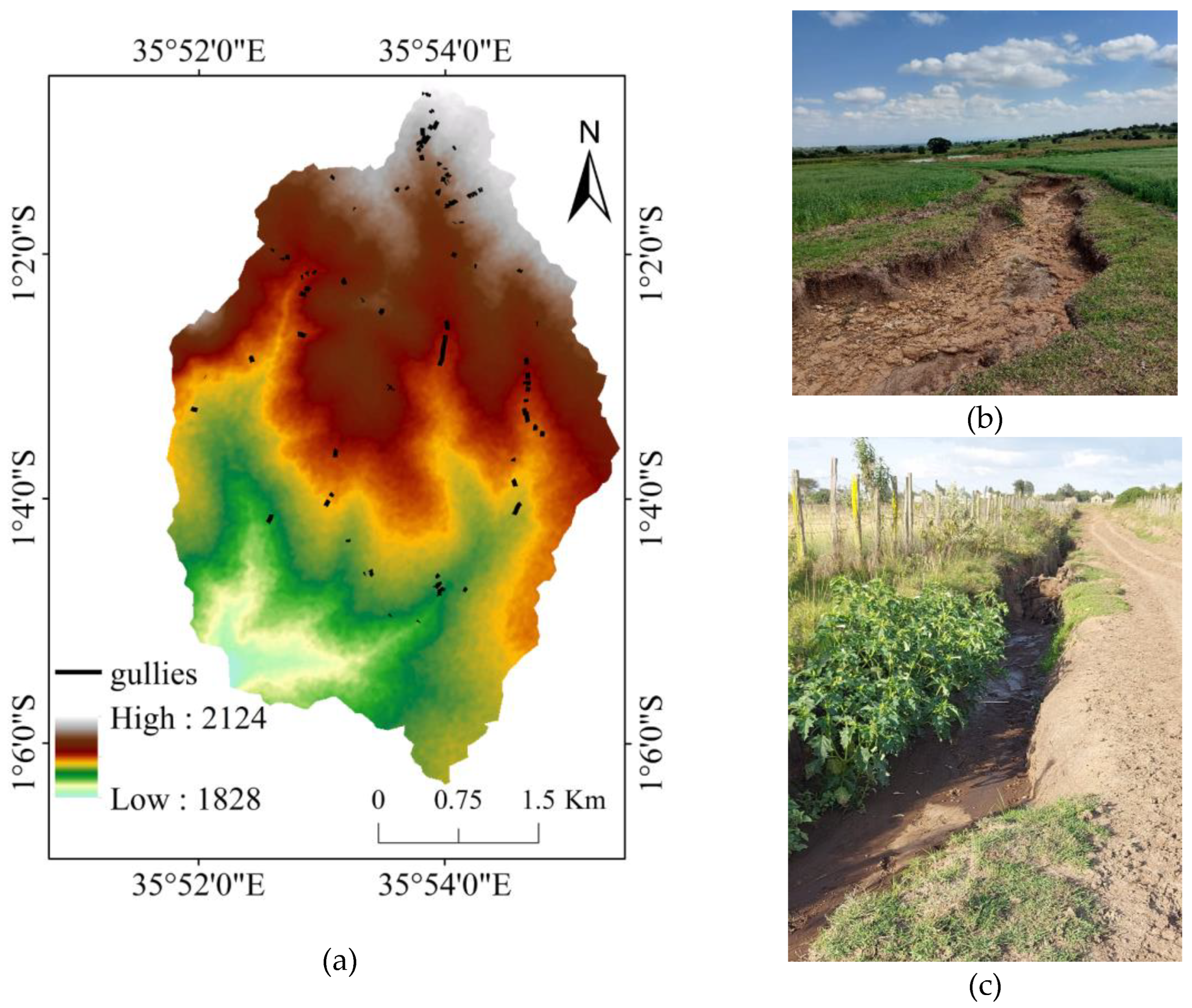
2.1. Study Area
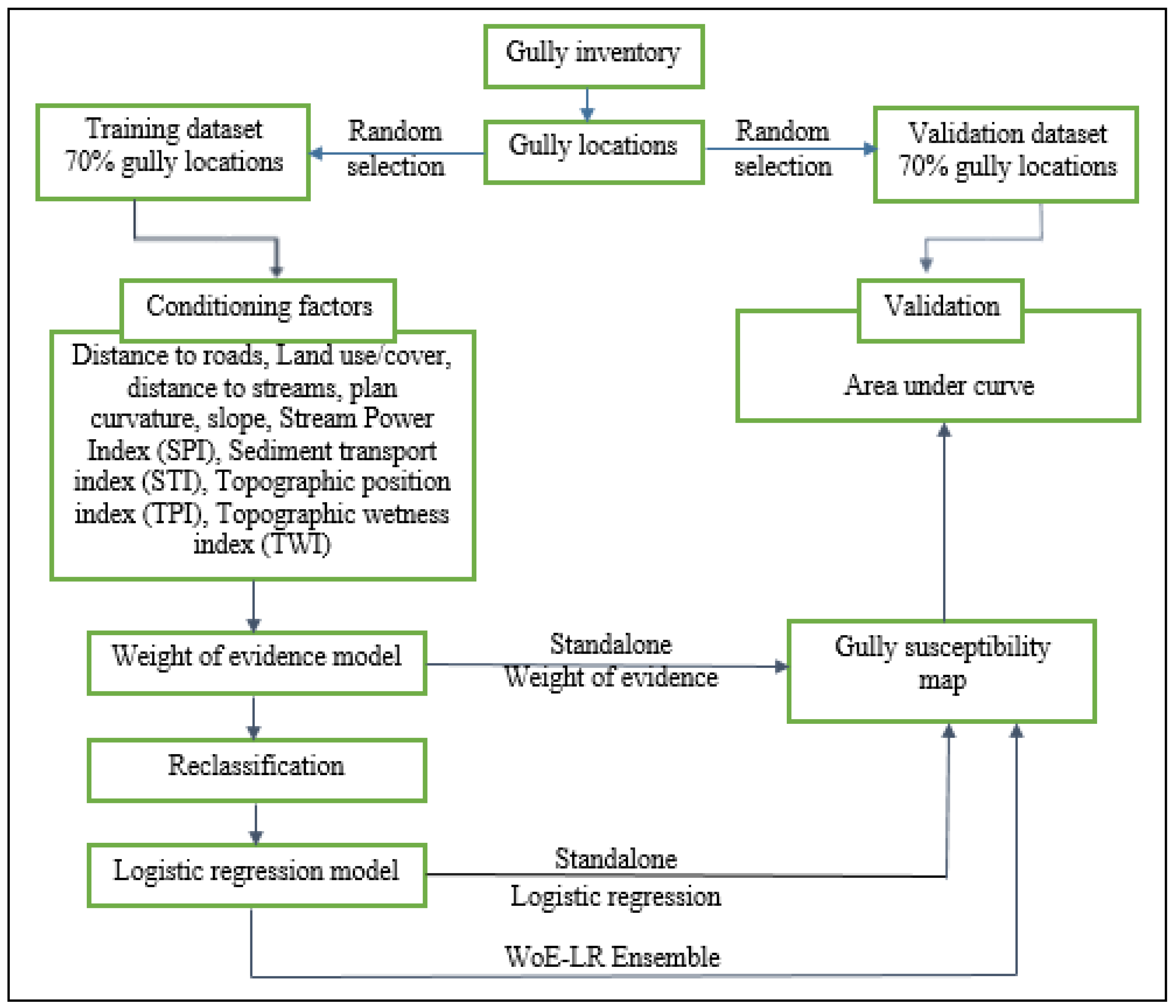
2.2. Methodology
2.2.1. Gully Erosion Inventory
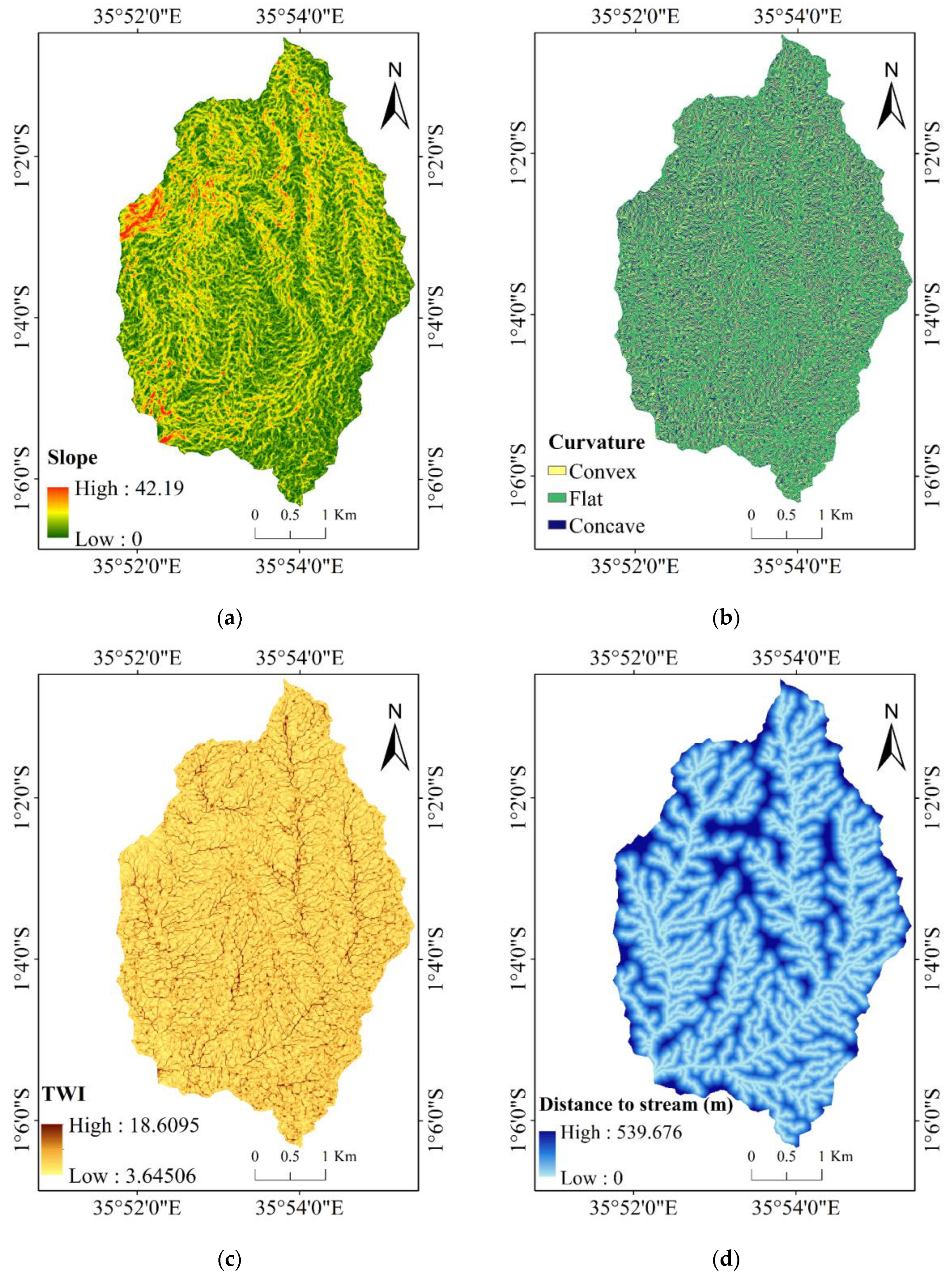
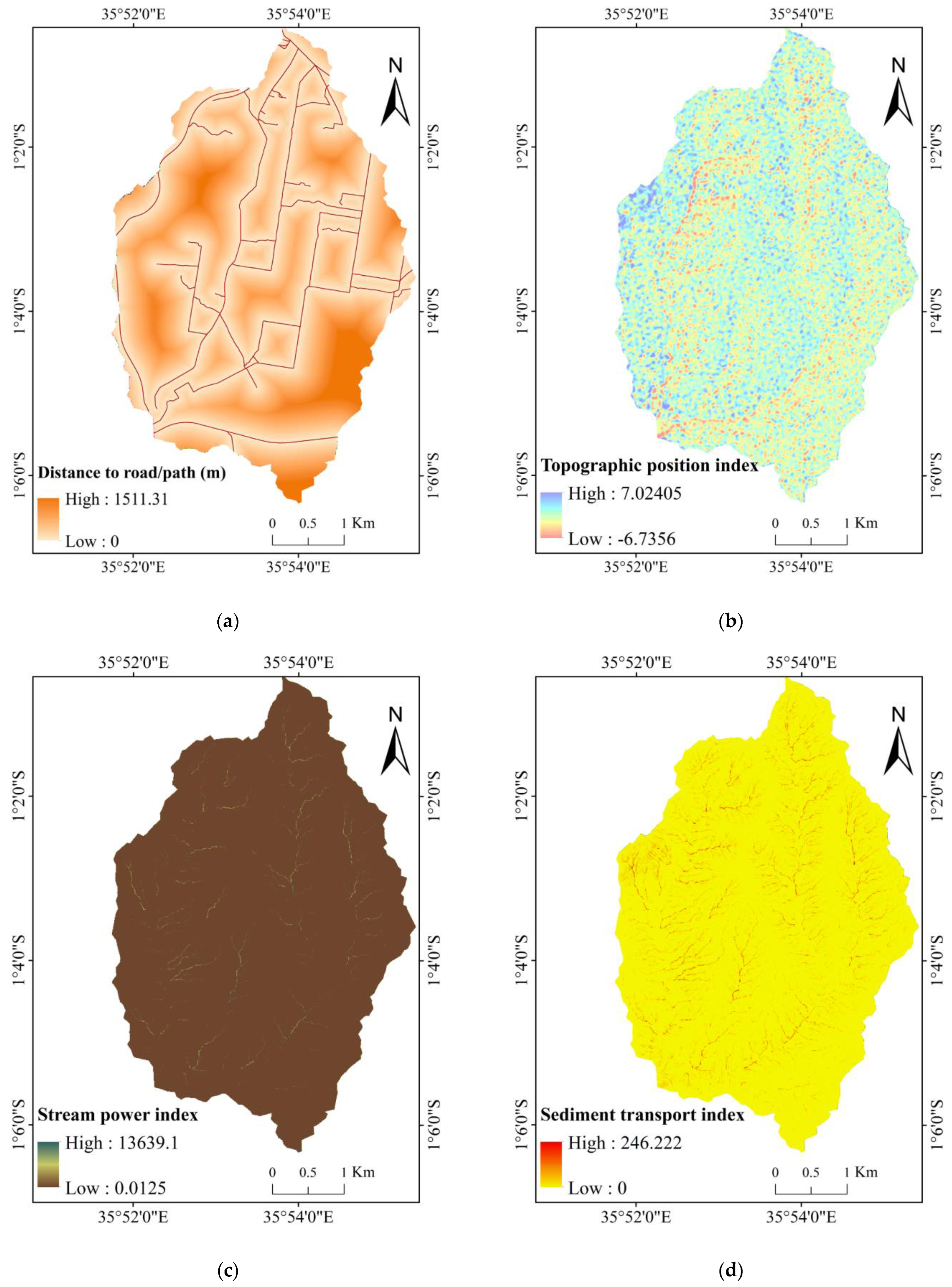
2.2.2. Conditioning Factors
2.3. Multi-Collinearity Test
2.4. Weight of Evidence Model
2.5. Logistic Regression Model
2.6. Model Evaluation
3. Results
3.1. Conditioning Factor’s Effect
3.1.1. Multicollinearity Test
3.1.2. Weight of Evidence Model
3.1.3. Logistic Regression Model
3.1.4. LR–WoE Ensemble Model
3.2. Gully Erosion Hazard
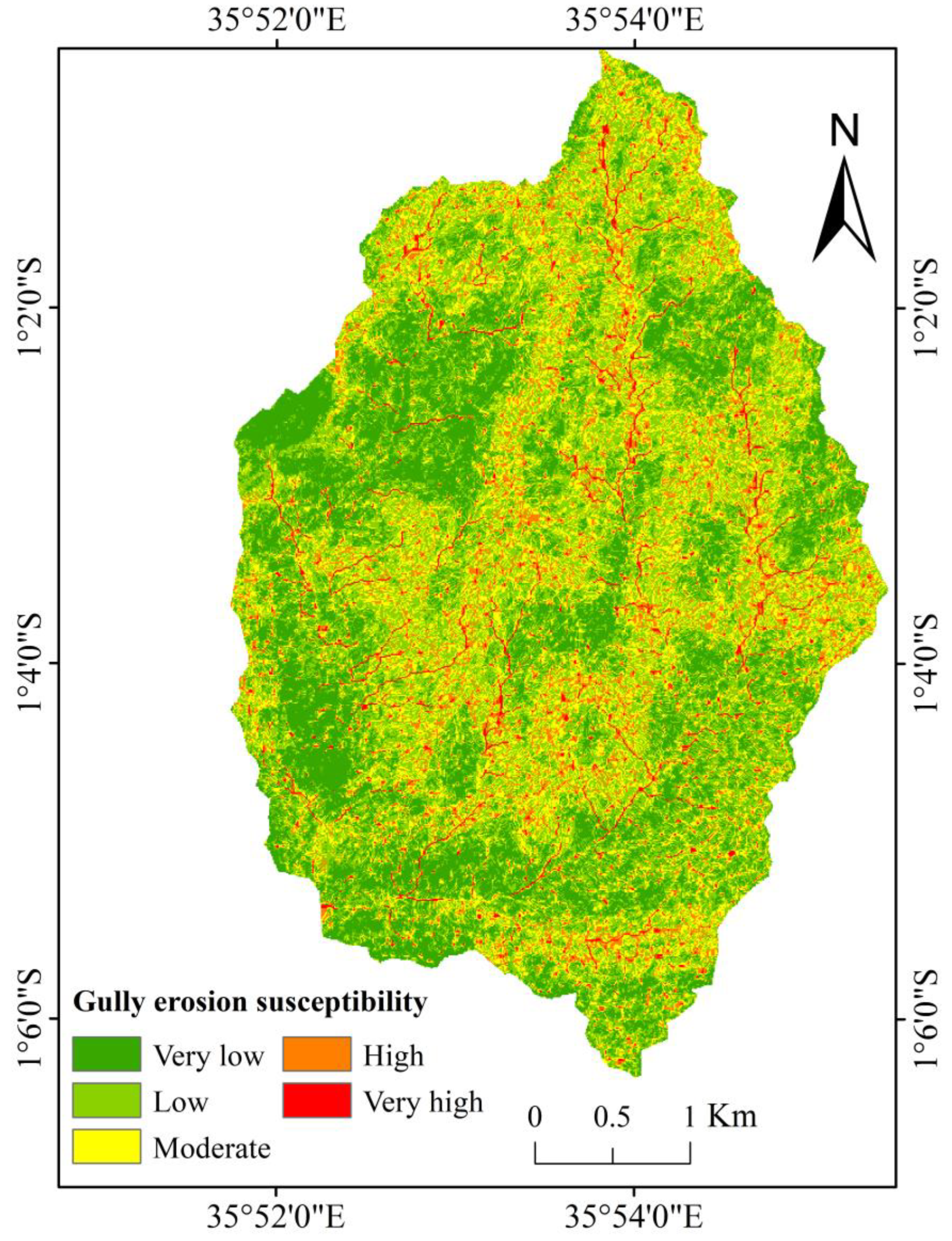
3.2.1. Weight of Evidence Model
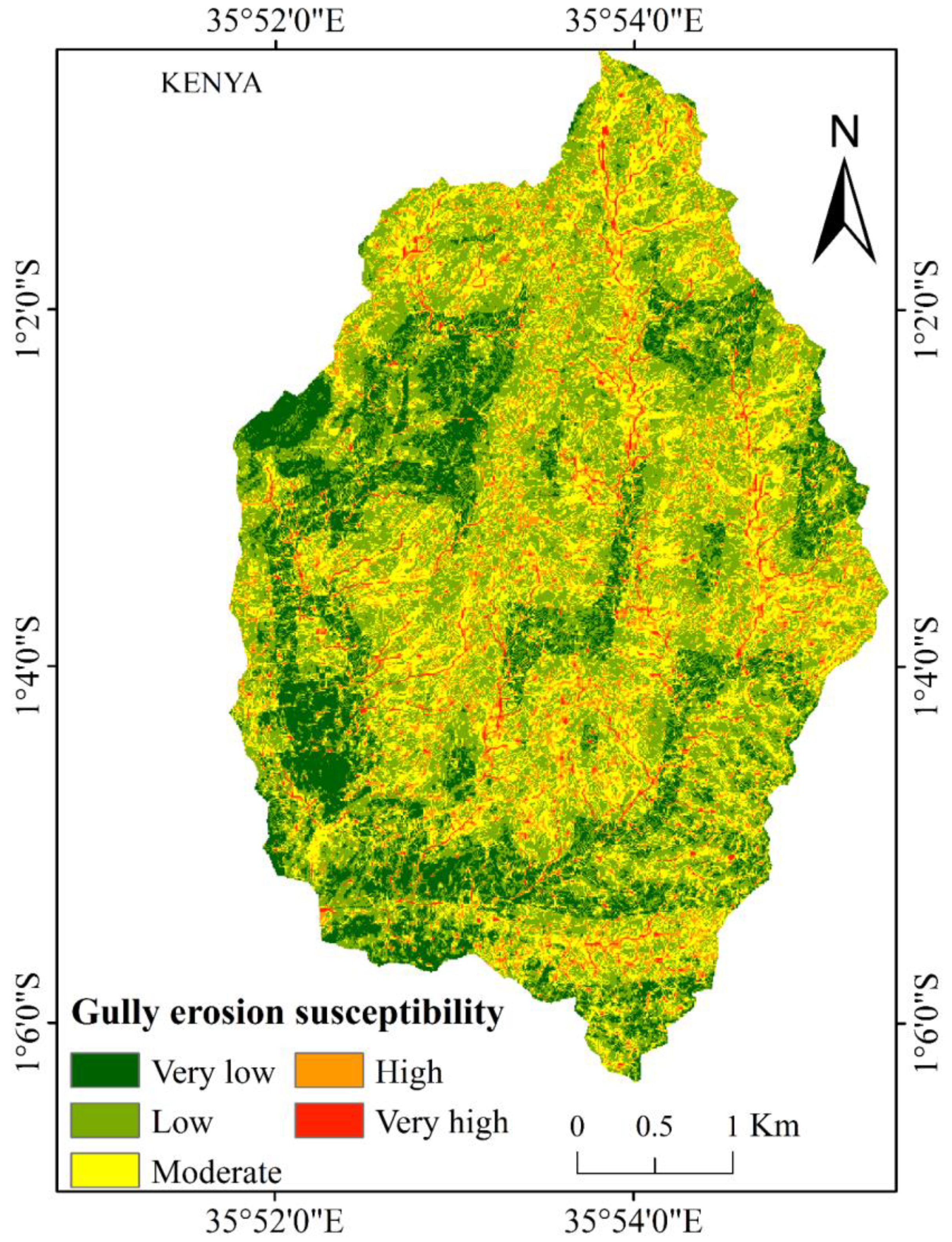
3.2.2. LR Model and WoE–LR Ensemble Model
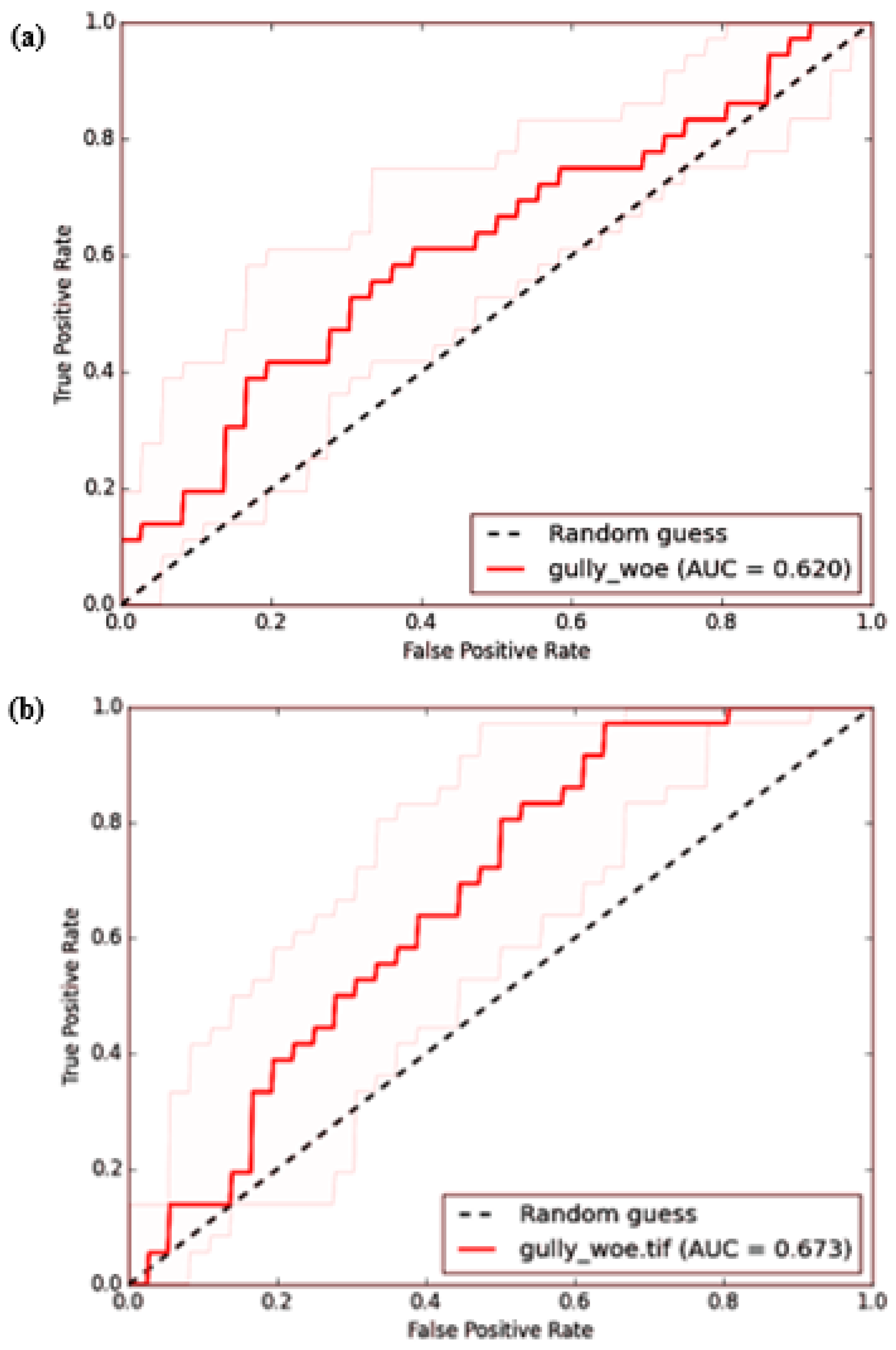
3.3. Model Validation
4. Discussion
5. Conclusions and Recommendations
Author Contributions
Funding
Data Availability Statement
Acknowledgments
Conflicts of Interest
References
- Arabameri, A.; Pradhan, B.; Pourghasemi, H.R.; Rezaei, K. Identification of erosion-prone areas using different multi-criteria decision-making techniques and gis. Geomat. Nat. Hazards Risk 2018, 9, 1129–1155. [Google Scholar] [CrossRef]
- Apollonio, C.; Petroselli, A.; Tauro, F.; Cecconi, M.; Biscarini, C.; Zarotti, C.; Grimaldi, S. Hillslope erosion mitigation: An experimental proof of a nature-based solution. Sustainability 2021, 13, 6058. [Google Scholar] [CrossRef]
- Sholagberu, A.T.; Mustafa, M.R.; Yusof, K.W.; Hashim, A.M. Geo-statistical based susceptibility mapping of soil erosion and optimization of its causative factors: A conceptual framework. J. Eng. Sci. Technol. 2017, 12, 2880–2895. [Google Scholar]
- Fox, G.A.; Sheshukov, A.; Cruse, R.; Kolar, R.L.; Guertault, L.; Gesch, K.R.; Dutnell, R.C. Reservoir Sedimentation and Upstream Sediment Sources: Perspectives and Future Research Needs on Streambank and Gully Erosion. Environ. Manag. 2016, 57, 945–955. [Google Scholar] [CrossRef]
- Zabihi, M.; Mirchooli, F.; Motevalli, A.; Darvishan, A.K.; Pourghasemi, H.R.; Zakeri, M.A.; Sadighi, F. Spatial modelling of gully erosion in Mazandaran Province, northern Iran. Catena 2018, 161, 1–13. [Google Scholar] [CrossRef]
- Odunuga, S.; Ajijola, A.; Igwetu, N.; Adegun, O. Land susceptibility to soil erosion in Orashi Catchment, Nnewi South, Anambra State, Nigeria. Proc. Int. Assoc. Hydrol. Sci. 2018, 376, 87–95. [Google Scholar] [CrossRef]
- Slimane, A.B.; Raclot, D.; Evrard, O.; Sanaa, M.; Lefevre, I.; Bissonnais, Y.L. Relative contribution of rill/interrill and gully/channel erosion to small reservoir siltation in mediterranean environments. Land Degrad. Dev. 2016, 27, 785–797. [Google Scholar]
- Issaka, S.; Ashraf, M.A. Impact of soil erosion and degradation on water quality: A review. Geol. Ecol. Landsc. 2017, 1, 1301053. [Google Scholar] [CrossRef]
- Borrelli, P.; Robinson, D.A.; Fleischer, L.R.; Lugato, E.; Ballabio, C.; Alewell, C.; Meusburger, K.; Modugno, S.; Schütt, B.; Ferro, V.; et al. An assessment of the global impact of 21st century land use change on soil erosion. Nat. Commun. 2017, 8, 1–13. [Google Scholar] [CrossRef]
- Hassen, G.; Bantider, A. Assessment of drivers and dynamics of gully erosion in case of Tabota Koromo and Koromo Danshe watersheds, South Central Ethiopia. Geoenviron. Disasters 2020, 7, 5. [Google Scholar] [CrossRef]
- Bui, D.T.; Shirzadi, A.; Shahabi, H.; Chapi, K.; Omidavr, E.; Pham, B.T.; Asl, D.T.; Khaledian, H.; Pradhan, B.; Panahi, M.; et al. A novel ensemble artificial intelligence approach for gully erosion mapping in a semi-arid watershed (Iran). Sensors 2019, 19, 2444. [Google Scholar] [CrossRef]
- Arabameri, A.; Pourghasemi, H.R. Spatial Modeling of Gully Erosion Using Linear and Quadratic Discriminant Analyses in GIS and R. In Spatial Modeling in GIS and R for Earth and Environmental Sciences; Elsevier: Amsterdam, The Netherlands, 2019; pp. 299–321. [Google Scholar] [CrossRef]
- Poesen, J.; Nachtergaele, J.; Verstraeten, G.; Valentin, C. Gully erosion and environmental change: Importance and research needs. Catena 2003, 50, 91–133. [Google Scholar] [CrossRef]
- Zakerinejad, R.; Maerker, M. An integrated assessment of soil erosion dynamics with special emphasis on gully erosion in the Mazayjan basin, southwestern Iran. Nat. Hazards 2015, 79, 25–50. [Google Scholar] [CrossRef]
- Arabameri, A.; Cerda, A.; Tiefenbacher, J.P. Spatial pattern analysis and prediction of gully erosion using novel hybrid model of entropy-weight of evidence. Water 2019, 11, 1129. [Google Scholar] [CrossRef]
- Angileri, S.E.; Conoscenti, C.; Hochschild, V.; Märker, M.; Rotigliano, E.; Agnesi, V. Water erosion susceptibility mapping by applying Stochastic Gradient Treeboost to the Imera Meridionale River Basin (Sicily, Italy). Geomorphology 2016, 262, 61–76. [Google Scholar] [CrossRef]
- Javidan, N.; Kavian, A.; Pourghasemi, H.R.; Conoscenti, C.; Jafarian, Z. Gully erosion susceptibility mapping using multivariate adaptive regression splines-replications and sample size scenarios. Water 2019, 11, 2319. [Google Scholar] [CrossRef]
- Conoscenti, C.; Angileri, S.; Cappadonia, C.; Rotigliano, E.; Agnesi, V.; Märker, M. Gully erosion susceptibility assessment by means of GIS-based logistic regression: A case of Sicily (Italy). Geomorphology 2014, 204, 399–411. [Google Scholar] [CrossRef]
- Han, F.; Ren, L.; Zhang, X.; Li, Z. The WEPP Model Application in a Small Watershed in the Loess Plateau. PLoS ONE 2016, 11, e0148445. [Google Scholar] [CrossRef]
- Langendoen, E.J.; Wells, R.R.; Ursic, M.E.; Vieira, D.A.N.; Dabney, S.M. Evaluating sediment transport capacity relationships for use in ephemeral gully erosion models. IAHS-AISH Proc. Rep. 2014, 367, 128–133. [Google Scholar] [CrossRef]
- Pourghasemi, H.R.; Yousefi, S.; Kornejady, A.; Cerdà, A. Performance assessment of individual and ensemble data-mining techniques for gully erosion modeling. Sci. Total Environ. 2017, 609, 764–775. [Google Scholar] [CrossRef]
- Wu, Z.; Wu, Y.; Yang, Y.; Chen, F.; Zhang, N.; Ke, Y.; Li, W. A comparative study on the landslide susceptibility mapping using logistic regression and statistical index models. Arab. J. Geosci. 2017, 10, 187. [Google Scholar] [CrossRef]
- Dube, F.; Nhapi, I.; Murwira, A.; Gumindoga, W.; Goldin, J.; Mashauri, D.A. Potential of weight of evidence modelling for gully erosion hazard assessment in Mbire District–Zimbabwe. Phys. Chem. Earth 2014, 67–69, 145–152. [Google Scholar] [CrossRef]
- Kornejady, A.; Ownegh, M.; Bahremand, A. Landslide susceptibility assessment using maximum entropy model with two different data sampling methods. Catena 2017, 152, 144–162. [Google Scholar] [CrossRef]
- Rahmati, O.; Haghizadeh, A.; Pourghasemi, H.R.; Noormohamadi, F. Gully erosion susceptibility mapping: The role of GIS-based bivariate statistical models and their comparison. Nat. Hazards 2016, 82, 1231–1258. [Google Scholar] [CrossRef]
- Rahmati, O.; Pourghasemi, H.R.; Melesse, A.M. Application of GIS-based data driven random forest and maximum entropy models for groundwater potential mapping: A case study at Mehran Region, Iran. Catena 2016, 137, 360–372. [Google Scholar] [CrossRef]
- Gómez-Gutiérrez, Á.; Conoscenti, C.; Angileri, S.E.; Rotigliano, E.; Schnabel, S. Using topographical attributes to evaluate gully erosion proneness (susceptibility) in two mediterranean basins: Advantages and limitations. Nat. Hazards 2015, 79, 291–314. [Google Scholar] [CrossRef]
- Jaafari, A.; Najafi, A.; Pourghasemi, H.R.; Rezaeian, J.; Sattarian, A. GIS-based frequency ratio and index of entropy models for landslide susceptibility assessment in the Caspian forest, northern Iran. Int. J. Environ. Sci. Technol. 2014, 11, 909–926. [Google Scholar] [CrossRef]
- Hong, H.; Chen, W.; Xu, C.; Youssef, A.M.; Pradhan, B.; Tien Bui, D. Rainfall-induced landslide susceptibility assessment at the Chongren area (China) using frequency ratio, certainty factor, and index of entropy. Geocarto Int. 2017, 32, 139–154. [Google Scholar] [CrossRef]
- Chen, W.; Pourghasemi, H.R.; Kornejady, A.; Zhang, N. Landslide spatial modeling: Introducing new ensembles of ANN, MaxEnt, and SVM machine learning techniques. Geoderma 2017, 305, 314–327. [Google Scholar] [CrossRef]
- Nhu, V.-H.; Mohammadi, A.; Shahabi, H.; Bin Ahmad, B.; Al-Ansari, N.; Shirzadi, A.; Clague, J.J.; Jaafari, A.; Chen, W.; Nguyen, H. Landslide Susceptibility Mapping Using Machine Learning Algorithms and Remote Sensing Data in a Tropical Environment. Int. J. Environ. Res. Public Health 2020, 17, 4933. [Google Scholar]
- Chen, W.; Li, H.; Hou, E.; Wang, S.; Wang, G.; Panahi, M.; Li, T.; Peng, T.; Guo, C.; Niu, C.; et al. GIS-based groundwater potential analysis using novel ensemble weights-of-evidence with logistic regression and functional tree models. Sci. Total Environ. 2018, 634, 853–867. [Google Scholar] [CrossRef]
- Roodposhti, M.S.; Safarrad, T.; Shahabi, H. Drought sensitivity mapping using two one-class support vector machine algorithms. Atmos. Res. 2017, 193, 73–82. [Google Scholar] [CrossRef]
- Shafizadeh-Moghadam, H.; Valavi, R.; Shahabi, H.; Chapi, K.; Shirzadi, A. Novel forecasting approaches using combination of machine learning and statistical models for flood susceptibility mapping. J. Environ. Manag. 2018, 217, 1–11. [Google Scholar] [CrossRef]
- Kadavi, P.R.; Lee, C.W.; Lee, S. Application of ensemble-based machine learning models to landslide susceptibility mapping. Remote Sens. 2018, 10, 1252. [Google Scholar] [CrossRef]
- Tehrany, M.S.; Pradhan, B.; Jebur, M.N. Flood susceptibility mapping using a novel ensemble weights-of-evidence and support vector machine models in GIS. J. Hydrol. 2014, 512, 332–343. [Google Scholar] [CrossRef]
- Tchouateu, O.T.; Mwangi, H.M.; Sang, J.K.; Ngugi, H.N. Impacts of climate change on peak streamflow in Kakia-Esamburmbur Sub-catchment of Enkare Narok River catchment, Kenya. J. Sustain. Res. Eng. 2020, 5, 194–205. [Google Scholar]
- Mireille, N.M.; Mwangi, H.M.; Mwangi, J.K.; Gathenya, J.M. Analysis of Land Use Change and Its Impact on the Hydrology of Kakia and Esamburmbur of the. Hydrology 2019, 6, 86. [Google Scholar] [CrossRef]
- Umukiza, E.; Raude, J.M.; Wandera, S.M.; Petroselli, A.; Gathenya, J.M. Impacts of Land Use and Land Cover Changes on Peak Discharge and Flow Volume in Kakia and Esamburmbur Sub-Catchments of Narok Town, Kenya. Hydrology 2021, 8, 82. [Google Scholar] [CrossRef]
- Rahmati, O.; Tahmasebipour, N.; Haghizadeh, A.; Pourghasemi, H.R.; Feizizadeh, B. Evaluation of different machine learning models for predicting and mapping the susceptibility of gully erosion. Geomorphology 2017, 298, 118–137. [Google Scholar] [CrossRef]
- Lombardo, L.; Cama, M.; Maerker, M.; Rotigliano, E. A test of transferability for landslides susceptibility models under extreme climatic events: Application to the Messina 2009 disaster. Nat. Hazards 2014, 74, 1951–1989. [Google Scholar] [CrossRef]
- Alaska Satellite Facility Data Search Vertex (2020). Available online: https://search.asf.alaska.edu/#/?dataset=ALOS (accessed on 29 January 2023).
- Arabameri, A.; Chen, W.; Loche, M.; Zhao, X.; Li, Y.; Lombardo, L.; Cerda, A.; Pradhan, B.; Bui, D.T. Comparison of machine learning models for gully erosion susceptibility mapping. Geosci. Front. 2019, 11, 1609–1620. [Google Scholar] [CrossRef]
- Hu, C.; Wright, A.L.; Lian, G. Estimating the Spatial Distribution of Soil Properties Using Environmental Variables at a Catchment Scale in the Loess Hilly Area, China. Int. J. Environ. Res. Public Heal. 2019, 16, 491. [Google Scholar] [CrossRef]
- Trigila, A.; Iadanza, C.; Esposito, C.; Scarascia-Mugnozza, G. Comparison of Logistic Regression and Random Forests techniques for shallow landslide susceptibility assessment in Giampilieri (NE Sicily, Italy). Geomorphology 2015, 249, 119–136. [Google Scholar] [CrossRef]
- Jenness, J. Topographic Position Index (tpi_jen.avx) Extension for ArcView 3.x, v. 1.2. Jenness Enterprises. 2006. Available online: http://www.jennessent.com/arcview/tpi.htm (accessed on 1 March 2023).
- Chen, W.; Pourghasemi, H.R.; Naghibi, S.A. Prioritization of landslide conditioning factors and its spatial modeling in Shangnan County, China using GIS-based data mining algorithms. Bull. Eng. Geol. Environ. 2018, 77, 611–629. [Google Scholar] [CrossRef]
- Meinhardt, M.; Fink, M.; Tünschel, H. Landslide susceptibility analysis in central Vietnam based on an incomplete landslide inventory: Comparison of a new method to calculate weighting factors by means of bivariate statistics. Geomorphology 2015, 234, 80–97. [Google Scholar] [CrossRef]
- Copernicus. Available online: https://scihub.copernicus.eu/ (accessed on 31 August 2020).
- Ozdemir, A. Using a binary logistic regression method and GIS for evaluating and mapping the groundwater spring potential in the Sultan Mountains (Aksehir, Turkey). J. Hydrol. 2011, 405, 123–136. [Google Scholar] [CrossRef]
- Chen, W.; Sun, Z.; Han, J. Landslide susceptibility modeling using integrated ensemble weights of evidence with logistic regression and random forest models. Appl. Sci. 2019, 9, 171. [Google Scholar] [CrossRef]
- Pourghasemi, H.R.; Moradi, H.R.; Fatemi Aghda, S.M. Landslide susceptibility mapping by binary logistic regression, analytical hierarchy process, and statistical index models and assessment of their performances. Nat. Hazards 2013, 69, 749–779. [Google Scholar] [CrossRef]
- Xu, C.; Xu, X.; Dai, F.; Xiao, J.; Tan, X.; Yuan, R. Landslide hazard mapping using GIS and weight of evidence model in Qingshui River watershed of 2008 Wenchuan earthquake struck region. J. Earth Sci. 2012, 23, 97–120. [Google Scholar] [CrossRef]
- Shit, P.K.; Bhunia, G.S.; Pourghasemi, H.R. Gully Erosion Susceptibility Mapping Based on Bayesian Weight of Evidence. Adv. Sci. Technol. Innov. 2020, 8, 133–146. [Google Scholar] [CrossRef]
- Chen, W.; Reza, H.; Seyed, P.; Naghibi, A. A comparative study of landslide susceptibility maps produced using support vector machine with different kernel functions and entropy data mining models in China. Bull. Eng. Geol. Environ. 2018, 77, 647–664. [Google Scholar] [CrossRef]
- Youssef, A.M.; Pourghasemi, H.R.; Pourtaghi, Z.S.; Al-Katheeri, M.M. Landslide susceptibility mapping using random forest, boosted regression tree, classification and regression tree, and general linear models and comparison of their performance at Wadi Tayyah Basin, Asir Region, Saudi Arabia. Landslides Landslides 2015, 13, 839–856. [Google Scholar] [CrossRef]
- Pourtaghi, Z.S.; Pourghasemi, H.R.; Rossi, M. Erratum to: Forest fire susceptibility mapping in the Minudasht forests, Golestan province, Iran. Environ. Earth Sci. 2015, 73, 1535. [Google Scholar] [CrossRef]
- Meliho, M.; Khattabi, A.; Mhammdi, N. A GIS-based approach for gully erosion susceptibility modelling using bivariate statistics methods in the Ourika watershed, Morocco. Environ. Earth Sci. 2018, 77, 655. [Google Scholar] [CrossRef]
- Mukai, S. Gully Erosion Rates and Analysis of Determining Factors: A Case Study from the Semi-arid Main Ethiopian Rift Valley. Land Degrad. Dev. 2016, 28, 602–615. [Google Scholar] [CrossRef]
- Chuma, G.B.; Mondo, J.M.; Ndeko, A.B.; Mugumaarhahama, Y.; Bagula, E.M.; Blaise, M.; Valérie, M.; Jacques, K.; Karume, K.; Mushagalusa, G.N. Forest cover affects gully expansion at the tropical watershed scale: Case study of Luzinzi in Eastern DR Congo. Trees For. People 2021, 4, 100083. [Google Scholar] [CrossRef]
- Kou, M.; Jiao, J.; Yin, Q.; Wang, N.; Wang, Z.; Li, Y.; Yu, W.; Wei, Y.; Yan, F.; Cao, B. Successional Trajectory Over 10Years of Vegetation Restoration of Abandoned Slope Croplands in the Hill-Gully Region of the Loess Plateau. Land Degrad. Dev. 2016, 27, 919–932. [Google Scholar] [CrossRef]
- Azareh, A.; Rahmati, O.; Rafiei-Sardooi, E.; Sankey, J.B.; Lee, S.; Shahabi, H.; Ahmad, B. Modelling gully-erosion susceptibility in a semi-arid region, Iran: Investigation of applicability of certainty factor and maximum entropy models. Sci. Total Environ. 2019, 655, 684–696. [Google Scholar] [CrossRef]
- Arabameri, A.; Pradhan, B.; Bui, D.T. Spatial modelling of gully erosion in the Ardib River Watershed using three statistical-based techniques. Catena 2020, 190, 104545. [Google Scholar] [CrossRef]


| Parameter | Collinearity statistics | |
|---|---|---|
| Tolerance | VIF | |
| Curvature | 0.85 | 1.17 |
| Distance to road | 0.83 | 1.20 |
| Distance to stream | 0.92 | 1.09 |
| Landcover | 0.94 | 1.06 |
| Slope | 0.88 | 1.14 |
| SPI | 0.96 | 1.04 |
| STI | 0.41 | 2.41 |
| TPI | 0.88 | 1.14 |
| TWI | 0.40 | 2.49 |
| Factors | Class | W+ | W- | Wfinal |
|---|---|---|---|---|
| Slope (%) | 0–4.4 | −0.8852 | 0.0099 | −0.8951 |
| 4.5–8.1 | −0.5559 | 0.0441 | −0.6000 | |
| 8.2–11.2 | −0.3376 | 0.0359 | −0.3735 | |
| 11.3–16.0 | −0.2115 | 0.1523 | −0.3638 | |
| 16.1–42.1 | 0.4138 | −0.3441 | 0.7579 | |
| Curvature | Concave | −0.1319 | 0.0420 | −0.1739 |
| flat | 0.1961 | −0.2273 | 0.4233 | |
| convex | −0.3327 | 0.0938 | −0.4266 | |
| TWI | 3–6.1 | −0.4293 | 0.2090 | −0.6383 |
| 6.1–7.7 | −0.1982 | 0.0832 | −0.2814 | |
| 7.7–9.6 | 0.0501 | −0.0105 | 0.0606 | |
| 9.6–11.8 | 0.4188 | −0.0441 | 0.4629 | |
| 11.8–18.7 | 1.8308 | −0.1672 | 1.9979 | |
| Distance to stream (m) | 0–38 | −0.2149 | 0.2410 | −0.4559 |
| 38–89 | −0.6371 | 0.1579 | −0.7949 | |
| 89–150 | 1.3807 | −0.3503 | 1.7310 | |
| 150–224 | −0.7861 | 0.0261 | −0.8122 | |
| 224–539 | −0.5384 | 0.0051 | −0.5434 | |
| Distance to road (m) | 0–204 | 3.8957 | −0.2429 | 4.1387 |
| 204–434 | 0.5204 | −0.0521 | 0.5725 | |
| 434–683 | −0.7537 | 0.1270 | −0.8807 | |
| 683–959 | −0.9306 | 0.2262 | −1.1568 | |
| 959–1511 | 0.0563 | −0.0442 | 0.1005 |
| Factors | Class | W+ | W− | Wfinal |
|---|---|---|---|---|
| TPI | −6.8–−1.5 | 0.4019 | −0.0427 | 0.4446 |
| −1.5–−0.5 | 0.2975 | −0.1021 | 0.3996 | |
| −0.5–0.5 | 0.0118 | −0.0067 | 0.0185 | |
| 0.5–1.6 | −0.3065 | 0.0890 | −0.3955 | |
| 1.6–7.1 | −0.8978 | 0.0529 | −0.9507 | |
| SPI | 0–160 | −0.1122 | 1.3792 | −1.4915 |
| 160–750 | −1.3833 | 0.0208 | −1.4041 | |
| 750–1925 | 2.1774 | −0.0437 | 2.2211 | |
| 1925–4120 | 3.9965 | −0.0769 | 4.0735 | |
| 4120–13640 | 2.9584 | −0.0065 | 2.9649 | |
| STI | 0–4 | −0.1340 | 0.6750 | −0.8090 |
| 4–11 | 0.2549 | −0.0254 | 0.2803 | |
| 11–27 | 1.0322 | −0.0511 | 1.0834 | |
| 27–60 | 1.7170 | −0.0346 | 1.7516 | |
| 60–247 | 1.7125 | −0.0056 | 1.7181 | |
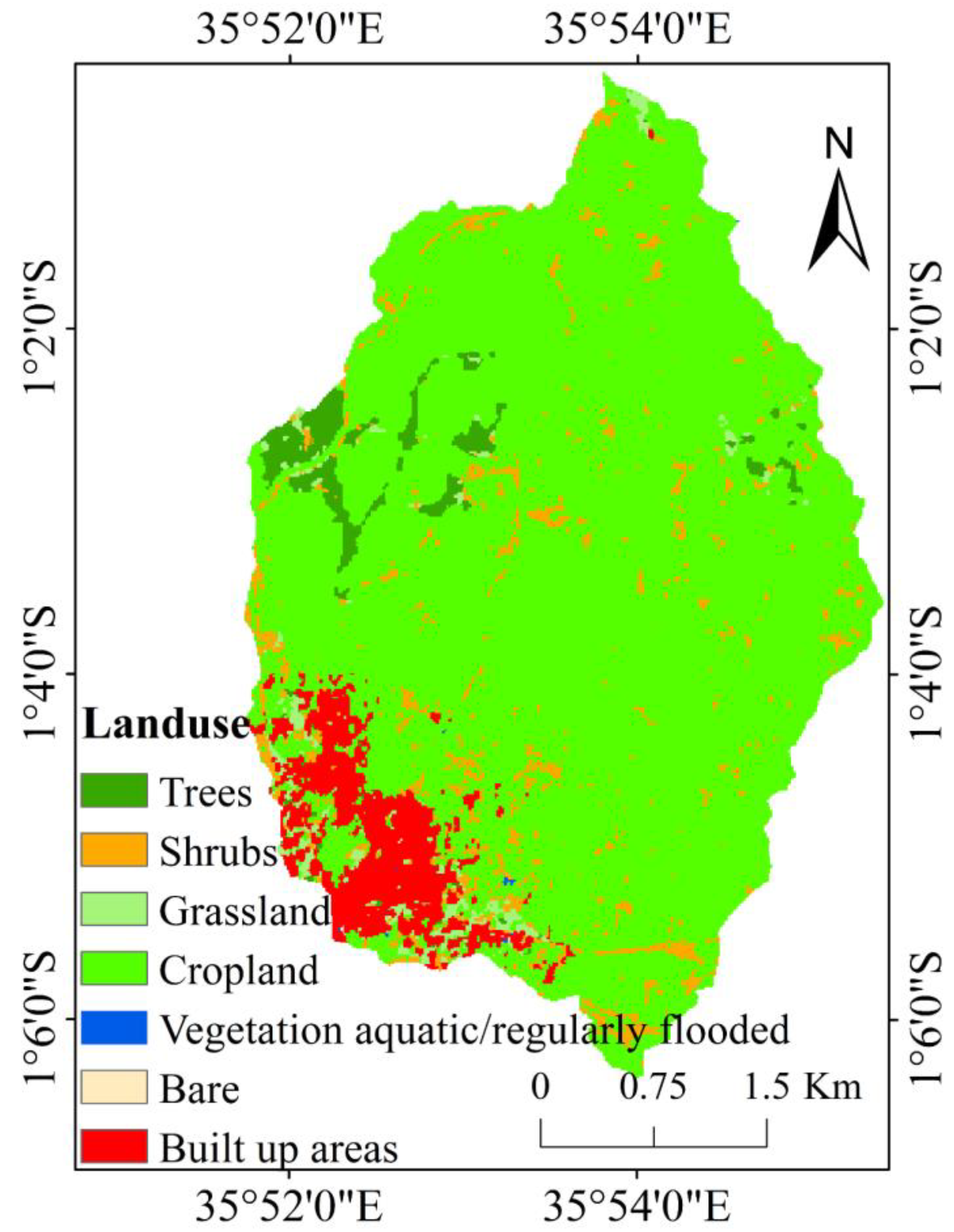
| LULC | Trees | −1.3375 | 0.0196 | −1.3570 |
| Shrubs | −0.9576 | 0.0343 | −0.9918 | |
| Grassland | −0.8827 | 0.0098 | −0.8925 | |
| Cropland | 0.1143 | −1.0517 | 1.1660 | |
| Vegetation aquatic/regularly flooded | 3.1360 | −0.0066 | 3.1425 | |
| Bare | 4.0024 | −0.0067 | 4.0091 | |
| Built-up areas | −2.1744 | 0.0553 | −2.2296 |
| Estimate | Standard Error | Z Value | Pr (>|z|) | ||
|---|---|---|---|---|---|
| (Intercept) | −7.025994 | 741.6681 | −0.009 | 0.99244 | |
| Curvature | −0.003545 | 0.002803 | −1.265 | 0.20593 | |
| Distance to road | 0.00677 | 0.001605 | 4.218 | 2.46 × 10⁻⁵ | *** |
| Distance to stream | 0.002653 | 0.001544 | 1.719 | 0.08569 | . |
| Land use/cover | 0.007804 | 0.003642 | 2.143 | 0.03214 | * |
| Slope | 0.004048 | 0.00634 | 0.639 | 0.52313 | |
| SPI | 0.008114 | 0.030244 | 0.268 | 0.78847 | |
| STI | −0.023267 | 0.006674 | −3.486 | 0.00049 | *** |
| TPI | −0.00194 | 0.002445 | −0.793 | 0.42765 | |
| TWI | 0.061095 | 0.014213 | 4.299 | 1.72 × 10⁻⁵ | *** |
Disclaimer/Publisher’s Note: The statements, opinions and data contained in all publications are solely those of the individual author(s) and contributor(s) and not of MDPI and/or the editor(s). MDPI and/or the editor(s) disclaim responsibility for any injury to people or property resulting from any ideas, methods, instructions or products referred to in the content. |
© 2023 by the authors. Licensee MDPI, Basel, Switzerland. This article is an open access article distributed under the terms and conditions of the Creative Commons Attribution (CC BY) license (https://creativecommons.org/licenses/by/4.0/).
Share and Cite
Nkonge, L.K.; Gathenya, J.M.; Kiptala, J.K.; Cheruiyot, C.K.; Petroselli, A. An Ensemble of Weight of Evidence and Logistic Regression for Gully Erosion Susceptibility Mapping in the Kakia-Esamburmbur Catchment, Kenya. Water 2023, 15, 1292. https://doi.org/10.3390/w15071292
Nkonge LK, Gathenya JM, Kiptala JK, Cheruiyot CK, Petroselli A. An Ensemble of Weight of Evidence and Logistic Regression for Gully Erosion Susceptibility Mapping in the Kakia-Esamburmbur Catchment, Kenya. Water. 2023; 15(7):1292. https://doi.org/10.3390/w15071292
Chicago/Turabian StyleNkonge, Lorraine K., John M. Gathenya, Jeremiah K. Kiptala, Charles K. Cheruiyot, and Andrea Petroselli. 2023. "An Ensemble of Weight of Evidence and Logistic Regression for Gully Erosion Susceptibility Mapping in the Kakia-Esamburmbur Catchment, Kenya" Water 15, no. 7: 1292. https://doi.org/10.3390/w15071292
APA StyleNkonge, L. K., Gathenya, J. M., Kiptala, J. K., Cheruiyot, C. K., & Petroselli, A. (2023). An Ensemble of Weight of Evidence and Logistic Regression for Gully Erosion Susceptibility Mapping in the Kakia-Esamburmbur Catchment, Kenya. Water, 15(7), 1292. https://doi.org/10.3390/w15071292